Abstract
In this paper, the macroscopic traffic states and network traffic dynamics during the Qingming Festival holiday are explored with the Macroscopic Fundament Diagram (MFD), including the weekday before the holiday (WBH), the day of Qingming Festival (DQF), and the ordinary weekday (OW). The network is heterogeneous on the densities’ distribution, and the congested areas are different in location and size. Normalized Cut (Ncut) algorithm is used to partition the heterogeneous network into multiple homogeneous subregions. The MFD of each subregion is distributed within the critical density on the WBH, and the high-density region moves from the city center to the periphery. On the DQF, high-density areas are on the central and west of the urban network. The congested branch appears on the MFD of the subregion. Then, two calibrated dynamic models, are applied to analyze the network evolution based on the partitioning results. On the basis of the calibrated model, several control strategies are proposed to relieve regional congestion on holidays. According to the simulation results, congestion on the DQF can be alleviated by controlling the external inflow ratio of subregion 2 or limiting the amount of traffic entering subregion 2 from the outside.
1. Introduction
During holidays (such as New Year’s Day, National Day), the travel behavior and pattern are different from those of ordinary weekdays, and the distribution of traffic on the urban network is heterogeneous [1,2]. It is essential to identify the congested area of the network and clarify the dynamic evolution characteristics. On this basis, control strategies for regional traffic flow could be implemented to relieve large-scale congestion. In recent years, the widespread collection and application of traffic data enables urban traffic flow to be analyzed on a large scale. Geroliminis and Daganzo [3] used the field data from Yokohama (Japan) to verify the existence of the Macroscopic Fundamental Diagram (MFD) in a real network, which provided a novel way for the study of network traffic flow. Later, different methods have been proposed to investigate the existence, characteristics, influencing factors of the MFD based on field data, theoretical analysis, and numerical simulations [4,5]. Moreover, several studies have been conducted to develop traffic management strategies based on the MFD [6]. The MFD describes the stable and reproducible relationship between the average flow, average density, and average speed of a network in a specific area. Take the advantage of the MFD, the states of network traffic flow can be predicted based on concise data. Furthermore, an important conclusion is derived that there is a constant ratio between the unit production and the rate at which cars reach their destinations, including cars leave the region along the perimeter and internally [3]. Based on this conclusion, the MFD could be explored for improving management and planning control strategies at the regional level.
With the aid of the MFD, the macroscopic characteristics and dynamic evolutions of traffic flow could be clarified [7], and perimeter control strategies could be designed to alleviate regional traffic congestions [8,9,10]. In terms of network dynamic evolution and equilibrium analysis, many studies constructed two-region [11,12] or multi-region [13,14] dynamic evolution models, theoretically analyzing the equilibrium and stability and revealing the impacts of heterogeneity on the MFD. Furthermore, in order to deal with traffic congestions among different regions, some macroscopic traffic models were proposed to study regional perimeter control [15,16,17]. The controllers were designed to manipulate the ratio of transfer flows on the borders of two neighbor regions. Studying two-region models, Geroliminis et al. [17] and Yang et al. [18] used the MFD to design the perimeter control and signal control strategy in the two-region system, which solved the traffic congestion problem in the core area and improved the mobility of the traffic flow in the region. Studying multi-region (more than two regions) models, Guo et al. [19] and Ding et al. [10] proposed a perimeter control for multiple regions to solve the problem of regional congestion and reduce the total delay of the network.
The aforementioned literature regarding the MFD mainly concentrated on ordinary weekdays or weekends, whereas studies focusing on specific holidays with some traditional activities have not been fully developed. In terms of data analysis, Shim et al. [20] observed distinct characteristics of the MFD on weekdays and weekends with the empirical data in the CBD of Daegu. The MFD showed a highly aggregated relationship on weekends, but exhibited bifurcations in a high-density state on weekdays. Wang et al. [21] analyzed the network data of Sendai City throughout one year and found that the characteristics of the MFD on weekdays and weekends were different. On weekdays, hysteresis loops appeared only in the morning and evening peaks, whereas a larger hysteresis loop appeared throughout the whole day on Saturday. On Sunday, there would be no hysteresis. Regarding the research on the network traffic flow characteristics during holidays, Shi et al. [22] investigated the MFD on expressways in Shanghai for one week (26 September to 1 October 2009, including the Chinese National Day) of different days. They also found two hysteresis loops in the morning and evening peaks on weekdays, while during the National Day, the hysteresis of the MFD had larger loops or different types.
Literature shows that the traffic flow characteristics and hysteresis types on public holidays are significantly different from those on weekdays and weekends. It is necessary to analyze the traffic characteristics from the macroscopic perspective of networks and develop control strategies to alleviate congestion during holidays. In many studies, the heterogeneity of density distribution is perceived as a critical factor that causes the hysteresis pattern [23,24]. For the heterogeneous network, Haddad et al. [15] introduced different control strategies with different levels of coordination for metropolitan transportation networks that have a hierarchical structure which consists of freeways and urban roads. Furthermore, some researchers proposed hierarchical control frameworks to investigate the dynamics of heterogeneity in urban regions, aiming at decreasing system delays and congestion heterogeneity [25,26].
In response to the issues mentioned above, this study analyzes the characteristics of regional traffic flow and the MFD on the network of Tianjin during the public holiday for Qingming Festival (1st to 4th April 2017), which is a traditional Chinese festival about ancestor worship and spring outings. The contribution of this paper is threefold. Firstly, the regional traffic flow characteristics are clarified based on the empirical data. The analysis involves different days, including the weekday before the holiday, during the holiday, and the day of Qingming Festival (the last day of the holiday). Secondly, the whole network is partitioned into several homogeneous subregions with different network densities and congestion levels. The calibrated dynamic models are applied to analyze the evolution process of traffic flow during the holidays. Finally, some control strategies are proposed to mitigate regional congestion during holidays based on the results of network state evolution under different model parameters.
2. Data Description and Network Partitioning
2.1. Data Description
The study area is the urban network of Tianjin, as shown in Figure 1, and the data are obtained from about 400 cameras on the network within the study area. The cameras are installed at the stop lines in each direction of most intersections, covering more than 80% of the network, and the data can represent the overall traffic states. The cameras continuously take pictures of vehicles passing through the stop lines of the intersection, records the ID and GPS coordinates of the camera, the license plate number, photographing time, and driving direction.
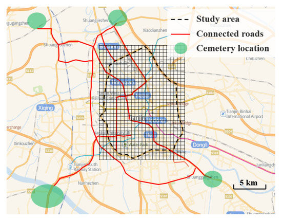
Figure 1.
Distribution of cemeteries and connecting roads in Tianjin.
During the public holiday for Qingming Festival, there are three days with no work. The first two days are generally leisure time for residents to travel to the countryside for spring. And the last day is the Qingming Festival. On the day, residents usually sweep cemeteries and worship ancestors in the morning. Several major cemeteries in Tianjin are distributed around the city center, and the connecting roads with the center are all expressways or arterial roads, as shown in Figure 1. On the day of Qingming Festival, the department of traffic management in Tianjin opened special bus lines from the city center to cemeteries. The departure time was between 6:00 and 7:30, and the return time was around 9:00. The traffic characteristics will be very different from the ordinary weekends due to multiple factors, such as the tomb-sweeping activities, spring outings, etc. Further, the data of ordinary weekdays are also analyzed for comparisons to explore the differences in traffic characteristics between holidays and ordinary weekdays.
2.2. Calculations of Network Traffic Variables
The characteristics and disciplines of the regional traffic flow are investigated by network traffic variables, including average flow, average speed, and average density. The network traffic variables are calculated using the average values over all lanes in the study area. The flow is obtained directly through the original data from the cameras, while the speed and the density are obtained by calculation.
Figure 2 is a schematic illustration of the position of the cameras. The data collected from two adjacent cameras along a link are used to calculate the traffic variables. In Figure 2, a pair of neighboring intersections is defined as a link with the length and the number of lanes . There are three upstream cameras (straight-direction camera , left-direction camera , and right-direction camera ) and one downstream camera . Define be the set of all links, . Link flows are counted at the downstream stop line of links and aggregated every 5 min as a period . Denote as the cumulative flow through the link in the period , and the network average flow is the mean value of all lanes covered by cameras in period [3], given as:
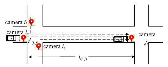
Figure 2.
Schematic illustration of the locations of cameras on a link.
The travel time for vehicle s passed link is the time difference between the two adjacent records on the link by license plate matching. Suppose there are vehicles passed through the link in period . The network average speed is calculated by the total distance and the total travel time [3], given as:
The network average density is denoted as , which is the ratio of the average flow and the average density:
2.3. Network Partitioning
The related research reveals [27] that the heterogeneous distribution of the network traffic flow has a significant impact on the MFD. Here the network is gridded to a size of 1 km × 1 km, and the density in each grid is calculated. Three days are considered, i.e., the weekday before the holiday (WBH), the day of Qingming Festival (DQF), and the ordinary weekday (OW). Figure 3 shows the comparisons in the network density distribution of these days. The traffic densities are heterogeneously distributed on the network, and the congested areas are different in location and size. On the WBH, the density in the city center is low, and the links with high densities are distributed on the suburb of the city (Figure 3a). The traffic flow on the DQF is mainly on the roads to cemeteries and its surrounding area (the west of the network in Figure 3b). On the OW, congestion is localized in the central area (Figure 3c). Therefore, it is necessary to divide the whole network into subregions with similar congestion levels, which provides a basis for further regional traffic control. Among graph segmentation methods, the normalized cut partition (Ncut) algorithm is commonly utilized due to its advantages effectiveness and robustness in the research of heterogeneous networks [28,29]. Therefore, the whole network is partitioned based on the link densities during 7:00–8:00 with congestion by Ncut algorithm. The basic idea is to partition the whole network into some subregions first and then merge them one by one; the details of the Ncut algorithm are given in Appendix A.
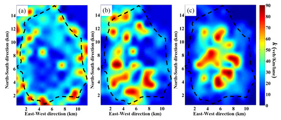
Figure 3.
Spatial–temporal distribution of network density during peak hour (7:00–8:00) on: (a) the weekday before the holiday, (b) the day of Qingming Festival, (c) the ordinary weekday.
The network densities during the peak hour are analyzed for the three days, i.e., the OW, the WBH, and the DQF. Figure 4 shows subregions by using the network partitioning on these days. The network is distinguished with different densities by partitioning. In Figure 4, the high-density area is labeled by red, the middle-density area is labeled by yellow, and the low-density area is labeled by green. The traffic density is similar within each subregion, while much distinct among different subregions. Table 1 lists the average density of each subregion and the evaluation indicators of partitioning.
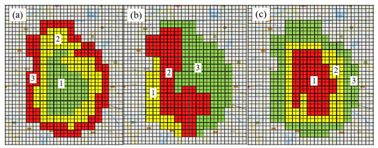
Figure 4.
Network subregions during peak periods on: (a) the weekday before the holiday, (b) the day of Qingming Festival, (c) the ordinary weekday. The numbers 1, 2 and 3 in each figure are the labels of the subregion, representing subregion1, subregion 2, and subregion 3, respectively.

Table 1.
Evaluation indicators of partitioning (The evaluation indicators of partitioning is defined as the average similarity , it is used to the evaluate the result of partitioning and calculated by Equation (A18) in Appendix A).
On the WBH and the OW, the network is partitioned into three annular subregions. The regions from the inner to the outer are labeled as subregion 1, 2, and 3. On the WBH, the high-density areas are located in the suburb (subregion 3 in Figure 4a), with an average density of 15.85 veh/km/lane, much smaller than the density (41.28 veh/km/lane) in the city center on the OW. And the average density of the two inner subregions is below 10 veh/km/lane. In contrast, on the DQF, the network is partitioned into three adjacent subregions. On the DQF, the high-density area is located on the connecting roads to the cemeteries (subregion 2 in Figure 4b), and the average density of subregion 2 is more than 40 veh/km/lane. The partitioning results are consistent with the spatial distribution of the average density on the network (Figure 3).
After partitioning, the MFD on each subregion can be studied. Figure 5, Figure 6 and Figure 7 show the MFD of each subregion on the WBH, the DQF, and the OW, respectively. In the figures, the red square scatters □ represent subregion 1, the blue triangle scatters Δ represent subregion 2, and the black circles ◦ represent subregion 3. The differences in the MFD of subregions for these days can be concluded as follows.
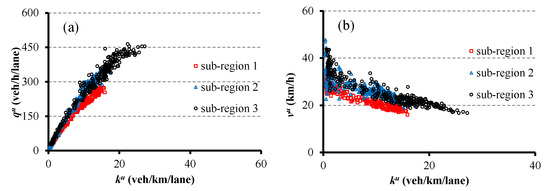
Figure 5.
MFD of subregions on the weekday before the holiday: (a) average flow-average density, (b) average speed-average density.
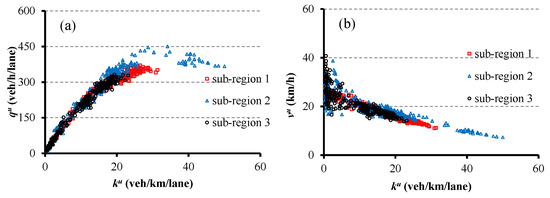
Figure 6.
MFD of subregions on the day of Qingming Festival: (a) average flow-average density, (b) average speed-average density.
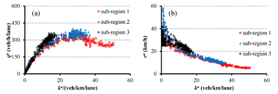
Figure 7.
MFD of subregions on the ordinary weekday: (a) average flow-average density, (b) average speed-average density.
- (1)
- The MFDs on the WBH and the OW are different (Figure 5 and Figure 7). Both days are weekdays, and the network is partitioned into three annular subregions. For subregions 1 and 2, the MFD on the WBH has no congested branch, while the congested branch appears on the MFD of the OW. On the WBH, the average densities of subregions 1 and 2 are much lower than those on the OW, reaching 50 and 37 veh/km/lane, respectively. In addition, the average speeds of all subregions on the WBH are above 16 km/h (□ and Δ in Figure 5b), while on the OW, the average speeds of subregions 1 and 2 decline significantly with the average density, and the minimal speeds are about 5.1 and 9.4 km/h (Figure 7b). On the OW, commuting trips are centralized during peak hours, resulting in congestion in the city center. The trips on the WBH are dispersed on the expressways in the suburb. Therefore, compared to that on the OW, the network average density is reduced on the WBH.
- (2)
- On the WBH (Figure 5), traffic states are all in free-flow branch with density less than 28 veh/km/lane, while a congested branch appears on the DQF (Δ in Figure 6a), where the average density approaches 50 veh/km/lane in subregion 2. The reason is that cemeteries are located in the west of the city, and a large amount of traffic flow on the DQF is squeezed into the roads to cemeteries in subregion 2.
- (3)
- The location and duration of congestion on the DQF are different from those on the OW. On the DQF, only a small number of scatters during 7:00–8:00 are distributed in the congested branches of the MFD, which correspond to the congestion period on the network. The average density increases and speed drops significantly in subregion 2 in a short time, resulting in congestion on the network about one hour. Due to the activities regarding tomb sweeping and ancestor worship on the DQF, the high-density area is localized in the west of the city. On the OW, more scatters during peak hours are distributed on the congested branch (Figure 7a) and the congestion lasts about 2–3 h. The congested areas are located in the central of the city.
In summary, due to differences in travel characteristics, the congestion level, location, and duration on the network during the holidays vary dramatically from those on weekdays. Therefore, it is necessary to design proper regional traffic control according to the different characteristics of each subregion on the network during the holidays.
3. Network Dynamic Evolution and Empirical Analysis
Based on the network partitioning in Section 2, two dynamic models are calibrated to analyze the regional traffic flow evolution based on the positional relationship of the subregions. The simulation results are compared with empirical data to confirm the validity of the models, and then regional control strategies are proposed based on the calibrated model and ground truth. Figure 8 depicts the construction of the models and regional control.
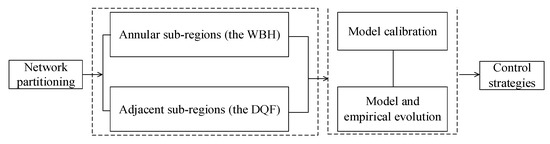
Figure 8.
The flow diagram of model construction and regional control.
3.1. The Model on the WBH
Based on the dynamic model [10,30], the data in this paper are used to calibrate the dynamic models for different days first, and then the models are applied to compare the effects of different control strategies.
3.1.1. Model Descriptions
Based on the network partitioning in Section 2, the network for the WBH consist of three annular subregions, and then is built as illustrated in Figure 9. Each subregion has its own MFD, and the average density of each region is (veh/km/lane). The MFD is expressed as Equation (4) [10]:
where, is the free-flow speed of subregion , (veh/km/lane) is the critical density of subregion , (veh/km/lane) is the jam density of the network, and is the backward speed of subregion . Assume that (veh/h/lane) is the transfer flow from subregion to
its neighbor subregion , (veh/h/lane) is the external inflow of subregion , and (veh/h/lane) is the outflow from subregion . There are linear relationships for the variables:
where, is the transfer ratio from subregion to subregion , is the average flow of subregion , is the external inflow ratio of subregion , and is the outflow ratio from subregion . is the maximal average flow of subregion .
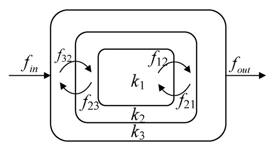
Figure 9.
The illustration of the model on the weekday before the holiday.
Typically, network state is defined by the average density of each subregion. If a subregion is not completely jammed, network state is determined by the external inflow, outflow, and transfer flow with other subregions. As the annular model has no external inflow and outflow of internal subregion 1 and 2, the inflow and the outflow of subregion 3 are the total. Subregions 1 and 3 do not lie adjacent, so there is no transfer flow between them. That is, , , , , . The network state evolution process can be described as follows:
where, is the average travel distance of subregion .
Substituting Equation (5) into Equation (6):
3.1.2. Model Calibration and Empirical Analysis
The MFD of each subregion on the two days in Figure 5 and Figure 7 is calibrated by empirical data. Generally, a congested branch will appear in the MFD where the average flow decreases as the density increases, and the density corresponding to the maximum flow is the critical density . For each network subregion of the WBH (Figure 5a) and subregion 3 of the OW (Figure 7a), no congested branch appears. The scatters on the MFD are all distributed within the critical density. Therefore, according to previous literature [31], the critical density of the MFD without a congested branch is calibrated as 30 veh/km/lane in this paper. The proportional relationship between the exit flow from the boundary and the flow inside the area appears to be a constant linear proportional trend after 6:00. The calibration results are listed in Table 2. The jam density is calculated as the average vehicle length of 5.2 m and the minimum headway distance of 1.95 m, veh/km/lane. The free-flow speed is the average value of the space-mean speed at night (0:00–5:00), that is km/h. The reason for the low free-flow speed is that the travel time included delays such as signal waiting and queuing at intersections. Moreover, the network of the study area includes different grades of roads, and the design speeds of sub-arterial roads and branches are lower than 40 km/h. There are also disturbances from non-motor vehicles and pedestrians that cause an increase in travel time. The space-mean average speed is the average of all vehicles on the network, and all these factors cause lower average speed.
Table 2.
Parameters calibration of the model on the weekday before the holiday and the ordinary weekday.
The calibrated model is used to simulate the evolution of the network state. Taking the average density at 7:00 of the network as the initial density, the initial densities of the network evolution are (4,6,10) veh/km/lane on the WBH, and are (24,19,4) veh/km/lane on the OW. Figure 10 shows the network evolution process over time on the WBH and the OW. Figure 10(a1) is the evolutions of subregions 1 and 2, and Figure 10(a2) is subregions 2 and 3 on the WBH, and Figure 10(b1,b2) are the evolutions on the OW. The blue line is the simulation result of the model, and the scatters are the empirical data. Points A and B represent the initial state and final state of the simulation, respectively. On the WBH, the state converges to a free-flow state in subregions 1 and 2, while it evolves to congestion in subregion 3. On the OW, both states in subregions 1 and 2 evolve to congested state over time. The simulation results are consistent with the ground truth, indicating that the model can reflect the actual evolution of the network. Compared with the OW, the traffic flow in the city center decreases on the WBH, the transfer ratio from subregion 2 to subregion 1 () decreases, and the congestion has not occurred in subregion 1. The transfer ratio and the external inflow ratio increase, leading to an increase in the traffic flow in subregion 3, and the network becomes congested.

Figure 10.
The network evolution of: (a1) subregions 1 and 2 on the weekday before the holiday, (a2) subregions 2 and 3 on the weekday before the holiday, (b1) subregions 1 and 2 on the ordinary weekday, (b2) subregions 2 and 3 on the ordinary weekday. The blue line is the simulation result of the model, and the arrow indicates the direction of system evolution. The blue scatters are the empirical data. Points A and B represent the initial state and final state of the simulation, respectively.
3.2. The Model on the DQF
3.2.1. Model Descriptions
The network is partitioned into three adjacent subregions on the DQF. Each one connects to the external system, which means each subregion has external inflow and outflow. The transfer ratio between subregion 1 and 3 is 0 (), as shown in Figure 11.
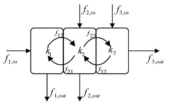
Figure 11.
The illustration of the model on the day of Qingming Festival.
The network state evolution process can be described as follows:
Substituting Equation (5) into Equation (8):
3.2.2. Model Calibration and Empirical Analysis
The MFD on the DQF in Figure 6 is also calibrated by empirical data. For subregion 2, veh/km/lane, and the scatters on the MFD of subregion 1 and 3 are distributed within the critical density, then veh/km/lane, veh/km/lane, veh/h/lane, veh/h/lane, and veh/h/lane. The calibration results of the transfer ratios, the external inflow ratio, and the outflow ratio are listed in Table 3.
Table 3.
Parameters calibration of the model on the day of Qingming Festival.
In simulation, the initial densities on the DQF are (4,3,2) veh/km/lane at 7:00, and the evolutions of the system over time are shown in Figure 12. Figure 12a is the evolutions of subregions 1 and 2, and Figure 12b is that of subregions 2 and 3. The blue line is the model simulation result, and the scatters are the empirical data. Points A and B represent the initial state and final state, respectively. Since the traffic flow is localized to the west of the urban network during the morning peak, the transfer ratio is significantly higher than those of other subregions. This leads to the network density of subregion 2 quickly exceeding the critical density and evolving toward congestion. The network states in subregions 1 and 3 are in free-flow state, and the model simulation results are consistent with the ground truth.
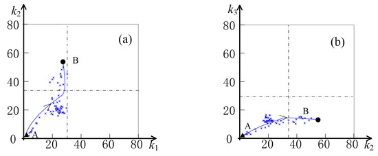
Figure 12.
The network evolution on the day of Qingming Festival: (a) subregions 1 and 2, (b) subregions 2 and 3. The blue line is the simulation result of the model, and the arrow indicates the direction of system evolution. The blue scatters are the empirical data. Points A and B represent the initial state and final state of the simulation, respectively.
4. Regional Control Strategies Analysis
Current literature has studied traffic control measures to relieve congestion, due to large amounts of trips and heterogeneous distribution of densities during holidays. In this study, the control strategies for a congested subregion mainly include two aspects: (1) to restrict vehicles from other regions entering the congested subregion, and (2) to guide vehicles from the congested subregion to other regions. It can be achieved by restricting vehicles from entering the congested subregion during peak hours or suggesting travelers avoid peak hours and guide navigation users to use other less crowded routes in real-time.
During the Qingming Festival holiday, the traffic flow of each subregion is in a free-flow state on the WBH, while the network state of subregion 2 is congested on the DQF. Therefore, the control strategies are designed for the DQF. Based on the calibrated models, some feasible control strategies are compared by simulations, and then proper control strategies are proposed to avoid large-scale network congestion.
4.1. Control Strategies for the DQF
The peak time for cemetery-sweeping of Qingming Festival is 7:00–8:00 during the morning, and the traffic flows from the east to west on the urban network. The model calibration results indicate that the transfer ratio from subregion 3 to subregion 2 in 7:00–8:00 is , and is during other periods. That is to say, the amount of traffic transfer from subregion 3 to subregion 2 during peak hours is much higher than that in other periods, causing that subregion 2 evolves to congestion. Therefore, the network density should be reduced by decreasing the inflow ratio or increasing the outflow ratio of subregion 2.
On the day of Qingming Festival, residents went to cemeteries from the urban area. Most of the demand for entering sub-region 2 is rigid, so it is difficult to reduce the total inflow to sub-region 2. In practical control, residents can be reminded to travel early or delay their travel time. By extending the control time, the total demand can be dispersed over time, avoiding concentrated travel in a short period to reduce the inflow ratio to sub-region 2. On the DQF, the control strategies for subregion 2 are designed as follows: (1) Strategy 1: decreasing or , which is to decrease the transfer ratio from subregion 1 to subregion 2 or decrease the external inflow ratio. (2) Strategy 2: increasing or , which is to increase the transfer ratio from subregion 2 to subregion 1 or increase the outflow ratio. The two control strategies limit vehicles entering subregion 2 and guide internal traffic flow away from the subregion, thus reducing the traffic density in subregion 2. The simulations under the two strategies are compared to analyze the impacts of different strategies on the network state.
4.2. Simulation Results
- (1)
- Strategy 1: decreasing or decreasing
Strategy 1 can be implemented by restricting vehicles entering subregion 2 from subregion 1 or outside. In simulations, the parameters and are decreased by 5% and 10%, respectively, to compare the impacts of different control strategies. Figure 13(a1,a2) display the network state evolution of the ground truth and after decreasing . The solid blue line is the evolution with no control, and the red and green dashed lines are the evolutions when being decreased by 5% and 10%. In the same simulation period, the evolution final points are B1, B2, and B3. The average density of subregion 2 has reduced, but the average density in subregion 1 has increased. The traffic state of subregion 1 evolves to congestion under decreasing by 10% (green line in Figure 13(a1)). It indicates that this strategy can alleviate the congestion of subregion 2 but cause subregion 1 in congestion. The simulation results of network state evolution under decreasing are shown in Figure 13(b1,b2). In this strategy, traffic state of each subregion is in free-flow state under decreasing by 10% (green line in Figure 13b). Thus, among the two strategies, decreasing strategy is better.
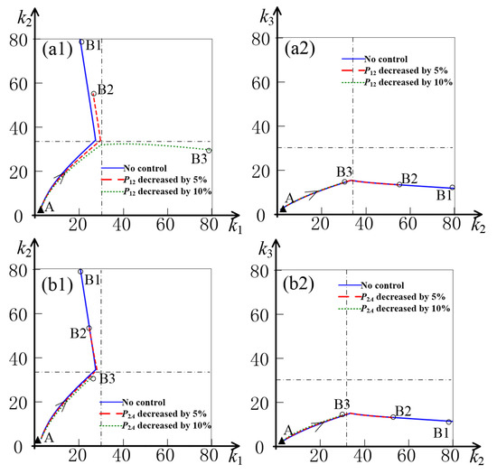
Figure 13.
The network evolution on the day of Qingming Festival: (a1) subregions 1 and 2, (a2) subregions 2 and 3 under is decreased, (b1) subregions 1 and 2, (b2) subregions 2 and 3 under is decreased. The line is the simulation result of the model, and the arrow indicates the direction of system evolution. Point A represents the initial state and points B1, B2, and B3 represent final state of the simulation under different control strategies.
- (2)
- Strategy 2: increasing or increasing
For the morning peak hours on the DQF, the outflow from subregion 2 can be increased by directing vehicles away from the region in time. In simulations, the parameters and are increased by 5% and 10%, respectively. The evolutions of the network are shown in Figure 14, where the solid blue line is the evolution with no control, and the red and green dashed lines are the evolutions under the two strategies. Points B1, B2, and B3 are final points in the same simulation period. Under increasing strategy, the average density of subregion 2 reduces with the increase in , but the traffic state of subregions 1 evolves to congestion. While under increasing strategy, the average density of subregion 2 decreases, and traffic states of subregions 1 and 2 are both in free-flow. Therefore, increasing strategy is better.
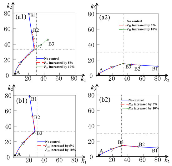
Figure 14.
The network evolution on the day of Qingming Festival: (a1) subregions 1 and 2, (a2) subregions 2 and 3 under is increased; (b1) subregions 1 and 2, (b2) subregions 2 and 3 under is increased. The line is the simulation result of the model, and the arrow indicates the direction of system evolution. Point A represents the initial state and points B1, B2, and B3 represent final state of the simulation under different control strategies.
In summary, when and are decreased or and are increased in the same proportion, controlling the external inflow or outflow ratio of subregion 2 is more effective in reducing the density of the regional network. To avoid a large amount of traffic gathering in this region in a short period, the total traffic flow can be dispersed in time, or plan detour routes for vehicles entering from outside, and implement temporary control upstream of the entrance. Since the roads connected to the cemeteries are mostly high-grade roads such as expressways and highways, the traffic flow can be limited at the entrances of expressways in actual traffic control.
5. Conclusions
This study analyzes the macroscopic traffic states during the Qingming Festival holiday, including the weekday before the holiday (WBH), the day of Qingming Festival (DQF), and the ordinary weekday (OW). The network densities distribution of these days are heterogeneous, and the congested areas are different in location and size. Based on the normalized cut (Ncut) algorithm, the network is partitioned into homogeneous subregions on different days and identifies the network congestion area on holidays. On the weekday before the holiday (WBH), the area with high density is in the suburb of the network, which is different from the ordinary weekday (OW). On the day of Qingming Festival (DQF), the congested areas distributed west on the network and subregion 2 is regional congestion during peak hours. Two dynamic models are calibrated to analyze the network evolution based on the partitioning results, and the simulation results of the calibrated model are consistent with the ground truth.
Based on the calibrated models, some proper control strategies are proposed to avoid or alleviate the regional network congestion on holidays. The results show that congestion on the DQF can be alleviated by controlling the external inflow ratio of subregion 2 or limiting the amount of traffic entering subregion 2 from the outside.
The study within this paper can identify the network congestion area at a macro level. Based on the MFD theory, the calibrated dynamic model is further used to investigate the mechanism of network state dynamic evolution. It provides a theoretical basis for proposing proper network macro-level control strategies to relieve regional congestion.
Author Contributions
Conceptualization, X.N.; methodology, X.N.; writing—original draft preparation, X.N.; writing—review and editing, X.Z. and D.X.; resources, J.B. All authors have read and agreed to the published version of the manuscript.
Funding
This research was funded by the National Natural Science Foundation of China (Grant No. 71771012, 71961137008, and 71931002).
Institutional Review Board Statement
Not applicable.
Informed Consent Statement
Not applicable.
Data Availability Statement
The data used in this paper are not publicly available.
Acknowledgments
The author would like to thank the anonymous reviewers for their valuable comments on the paper.
Conflicts of Interest
The authors declare no conflict of interest.
Appendix A
The partitioning algorithm refers to the research of Ji and Gerolimini [28], and the specific steps are as follows.
- (1)
- Initial partitioning of Ncut
The network is constructed as an undirected graph , the set of nodes is , and each node corresponds to a grid on the network, . In each grid, the mean of link densities is used as the density of the grid, . The spatial connectivity between the grids is defined by the adjacency matrix (the value is 0 or 1) is obtained. If grid and grid are adjacent, ; otherwise, . The spatial distance between two grids is defined as the shortest path between nodes and , which is the minimum number of grids from to on the graph. The similarity function between grid and is defined as follows:
Suppose the network is partitioned into subregion and , the total similarity between and can be expressed as:
where is the grid of the network . Then define the total disassociation between two subregions and the association within in each subregion are given as follows:
Ncut algorithm aims at minimizing between each subregion and maximizing within each subregion. That is to say that Equation (A3) reaches the minimum and Equation (A4) is the maximum. in Equation (A3) and in Equation (A4) have the relationship:
Therefore, the Ncut algorithm is used to minimize , which can simultaneously maximize the total disassociation between different subregions and the association within a subregion. Solving the problem is an NP-complete problem. Shi and Malik [29] proposed the equivalent eigenvalue system to partition the eigenvector corresponding to the second smallest eigenvalue.
- (2)
- Merging and evaluation indicators for partitioning
After the initial partitioning, the network is partitioned into several subregions with similar densities. A region with a higher degree of similarity is possibly divided since each subregion always is divided into two parts at each iteration step. Therefore, merging is necessary to improve the rationality of partitioning further. In the merging process, the average density differences in all two adjacent subregions are calculated. The two subregions with the smallest difference are merged until the evaluation indicators introduced in the next step are optimized.
Suppose that the whole network is partitioned into subregions. The indicator is defined to evaluate the difference between the two subregions:
where and are the number of grids in subregion and . To make sure the highest internal similarity and low similarity with other subregions, the following self-similarity can be used:
where , is the set of the subregions adjacent to subregion A in space. If , subregion A is properly partitioned. The overall partitioning can be evaluated by the value of the average similarity :
where is the set of subregions and is the number of subregions partitioned. The optimal partitioning result is obtained when reaches the minimum.
References
- Wang, B.B. Reconstruction and Evolution Analysis of Holiday Activity Chain under Integrated Multimodal Travel Information Service. Ph.D. Thesis, Beijing Jiaotong University, Beijing, China, 2017. [Google Scholar]
- Watanabe, H.; Chikaraishi, M.; Maruyama, T. How different are daily fluctuations and weekly rhythms in time-use behavior across urban settings? A case in two Japanese cities. Travel Behav. Soc. 2020, 22, 146–154. [Google Scholar] [CrossRef]
- Geroliminis, N.; Daganzo, C.F. Existence of urban-scale macroscopic fundamental diagrams: Some experimental findings. Transp. Res. Part B Methodol. 2008, 42, 759–770. [Google Scholar] [CrossRef]
- Leclercq, L.; Geroliminis, N. Estimating MFDs in simple networks with route choice. Transp. Res. Part B Methodol. 2013, 57, 468–484. [Google Scholar] [CrossRef]
- Gonzales, E.J.; Chavis, C.; Li, Y.; Daganzo, C.F. Multimodal Transport Modeling for Nairobi, Kenya: Insights and Recommendations with an Evidence Based Model; UC Berkeley Center for Future Urban Transport: Berkeley, CA, USA, 2009. [Google Scholar]
- Keyvan-Ekbatani, M.; Yildirimoglu, M.; Geroliminis, N.; Papageorgiou, M. Multiple Concentric Gating Traffic Control in Large-Scale Urban Networks. IEEE Trans. Intell. Transp. Syst. 2015, 16, 2141–2154. [Google Scholar] [CrossRef]
- Daganzo, C.F.; Geroliminis, N. An analytical approximation for the macroscopic fundamental diagram of urban traffic. Transp. Res. Part B Methodol. 2008, 42, 771–781. [Google Scholar] [CrossRef]
- Zheng, N.; Geroliminis, N. On the distribution of urban road space for multimodal congested networks. Transp. Res. Part B Methodol. 2013, 57, 326–341. [Google Scholar] [CrossRef]
- Gayah, V.V.; Gao, X.; Nagle, A.S. On the impacts of locally adaptive signal control on urban network stability and the macroscopic fundamental diagram. Transp. Res. Part B Methodol. 2014, 70, 255–268. [Google Scholar] [CrossRef]
- Ding, H.; Guo, F.; Zheng, X.; Zhang, W. Traffic guidance–perimeter control coupled method for the congestion in a macro network. Transp. Res. Part C Emerg. Technol. 2017, 81, 300–316. [Google Scholar] [CrossRef]
- Haddad, J.; Geroliminis, N. On the stability of traffic perimeter control in two-region urban cities. Transp. Res. Part B Methodol. 2012, 46, 1159–1176. [Google Scholar] [CrossRef]
- Daganzo, C.F.; Gayah, V.V.; Gonzales, E.J. Macroscopic relations of urban traffic variables: Bifurcations, multivaluedness and instability. Transp. Res. Part B Methodol. 2011, 45, 278–288. [Google Scholar] [CrossRef]
- Xie, D.-F.; Wang, D.Z.; Gao, Z.-Y. Macroscopic analysis of the fundamental diagram with inhomogeneous network and instable traffic. Transp. A Transp. Sci. 2015, 12, 20–42. [Google Scholar] [CrossRef]
- Zhong, R.; Xiong, J.; Huang, Y.; Sumalee, A.; Chow, A.H.F.; Pan, T. Dynamic System Optimum Analysis of Multi-Region Macroscopic Fundamental Diagram Systems with State-Dependent Time-Varying Delays. IEEE Trans. Intell. Transp. Syst. 2020, 21, 4000–4016. [Google Scholar] [CrossRef]
- Haddad, J.; Ramezani, M.; Geroliminis, N. Cooperative traffic control of a mixed network with two urban regions and a freeway. Transp. Res. Part B Methodol. 2013, 54, 17–36. [Google Scholar] [CrossRef]
- Keyvan-Ekbatani, M.; Kouvelas, A.; Papamichail, I.; Papageorgiou, M. Exploiting the fundamental diagram of urban networks for feedback-based gating. Transp. Res. Part B Methodol. 2012, 46, 1393–1403. [Google Scholar] [CrossRef]
- Geroliminis, N.; Haddad, J.; Ramezani, M. Optimal Perimeter Control for Two Urban Regions with Macroscopic Fundamental Diagrams: A Model Predictive Approach. IEEE Trans. Intell. Transp. Syst. 2012, 14, 348–359. [Google Scholar] [CrossRef]
- Yang, K.; Zheng, N.; Menendez, M. Multi-scale perimeter control approach in a connected-vehicle environment. Transp. Res. Part C Emerg. Technol. 2018, 94, 32–49. [Google Scholar] [CrossRef]
- Guo, Y.; Yang, L.; Gao, J. Coordinated Perimeter Control for Multiregion Heterogeneous Networks Based on Optimized Transfer Flows. Math. Probl. Eng. 2020, 2020, 3926265. [Google Scholar] [CrossRef]
- Shim, J.; Yeo, J.; Lee, S.; Hamdar, S.H.; Jang, K. Empirical evaluation of influential factors on bifurcation in macroscopic fundamental diagrams. Transp. Res. Part C Emerg. Technol. 2019, 102, 509–520. [Google Scholar] [CrossRef]
- Wada, K.; Akamatsu, T.; Hara, Y. An empirical analysis of macroscopic fundamental diagrams for Sendai road networks. Interdiscip. Inf. Sci. 2015, 21, 49–61. [Google Scholar]
- Shi, X.; Lin, H. Research on the Macroscopic Fundamental Diagram for Shanghai urban expressway network. Transp. Res. Procedia 2017, 25, 1300–1316. [Google Scholar] [CrossRef]
- Mazloumian, A.; Geroliminis, N.; Helbing, D. The spatial variability of vehicle densities as determinant of urban network capacity. Philos. Trans. R. Soc. A Math. Phys. Eng. Sci. 2010, 368, 4627–4647. [Google Scholar] [CrossRef]
- Saberi, M.; Mahmassani, H.S. The spatial variability of vehicle densities as determinant of urban network capacity. Transp. Res. Rec. J. Transp. Res. Board 2013, 3141, 44–56. [Google Scholar] [CrossRef]
- Ramezani, M.; Haddad, J.; Geroliminis, N. Dynamics of heterogeneity in urban networks: Aggregated traffic modeling and hierarchical control. Transp. Res. Part B Methodol. 2015, 74, 1–19. [Google Scholar] [CrossRef]
- Yildirimoglu, M.; Sirmatel, I.I.; Geroliminis, N. Hierarchical control of heterogeneous large-scale urban road networks via path assignment and regional route guidance. Transp. Res. Part B Methodol. 2018, 118, 106–123. [Google Scholar] [CrossRef]
- Geroliminis, N.; Sun, J. Properties of a well-defined macroscopic fundamental diagram for urban traffic. Transp. Res. Part B Methodol. 2011, 45, 605–617. [Google Scholar] [CrossRef]
- Ji, Y.; Geroliminis, N. On the spatial partitioning of urban transportation networks. Transp. Res. Part B Methodol. 2012, 46, 1639–1656. [Google Scholar] [CrossRef]
- Shi, J.; Malik, J. Normalized cuts and image segmentation. IEEE Trans. Pattern Anal. Mach. Intell. 2000, 22, 888–905. [Google Scholar]
- Gayah, V.V.; Daganzo, C.F. Clockwise hysteresis loops in the Macroscopic Fundamental Diagram: An effect of network instability. Transp. Res. Part B Methodol. 2011, 45, 643–655. [Google Scholar] [CrossRef]
- Ding, H.; Zhu, L.; Jiang, C.; Zheng, X. Traffic State Identification for Freeway Network Based on MFD. J. Chongqing Jiaotong Univ. (Nat. Sci.) 2018, 37, 77–83. [Google Scholar]
Disclaimer/Publisher’s Note: The statements, opinions and data contained in all publications are solely those of the individual author(s) and contributor(s) and not of MDPI and/or the editor(s). MDPI and/or the editor(s) disclaim responsibility for any injury to people or property resulting from any ideas, methods, instructions or products referred to in the content. |
© 2023 by the authors. Licensee MDPI, Basel, Switzerland. This article is an open access article distributed under the terms and conditions of the Creative Commons Attribution (CC BY) license (https://creativecommons.org/licenses/by/4.0/).