Comparison between Machine Learning and Physical Models Applied to the Evaluation of Co-Seismic Landslide Hazard

Abstract

A comparative methodology between advanced statistical tools and physical-based methods is carried out to ensure their reliability and objectivity for the evaluation of co-seismic landslide hazard maps. To do this, an inventory of landslides induced by the 2011 Lorca earthquake is used to highlight the usefulness of these methods to improve earthquake-induced landslide hazard analyses. Various statistical models, such as logistic regression, random forest, artificial neural network, and support vector machine, have been employed for co-seismic landslide susceptibility mapping. The results demonstrate that machine learning techniques using principal components (especially, artificial neural network and support vector machine) yield better results compared to other models. In particular, random forest shows poor results. Artificial neural network and support vector machine approaches are compared to the results of physical-based methods in the same area, suggesting that machine learning methods can provide better results for developing co-seismic landslide susceptibility maps. The application of different advanced statistical models shows the need for validation with an actual inventory of co-seismic landslides to ensure reliability and objectivity. In addition, statistical methods require a great amount of data. The results establish effective land planning and hazard management strategies in seismic areas to minimize the damage of future co-seismic landslides.

1. Introduction

There is a wide variety of phenomena that can trigger slope instabilities (landslides or rock falls), such as intense rainfall, rapid snowmelt, human-induced activities, or seismic events. These phenomena affect many areas of the world and are highly newsworthy, particularly those triggered by the seismic action of earthquakes, due to their great destructive potential. At present, the losses due to earthquake damage are difficult to approximate. Traditional methodologies estimate such damage costs based on building repair/reconstruction, without valuing economic losses due to the loss of economic activity and human lives [1]. Therefore, minimizing the effects and phenomena associated with strong ground motions is needed to characterize seismic hazards in inhabited regions. This is performed based on the study of past events and the geological and geotechnical conditions of areas that are likely to experience a seismic event, so that the inherent seismic hazard can be estimated.

Co-seismic landslides, as secondary effects of earthquakes [2], play a crucial role in identifying past seismic events and in improving seismic hazard predictions. These landslides provide valuable real-time geological evidence, allowing scientists to reconstruct the seismic catalog of a region and gain a better understanding of past seismic activity [3]. By expanding the dataset available for seismic analysis, greater accuracy in seismic hazard predictions can be achieved, which in turn contributes to strengthening community resilience against future seismic events.

The 2011 Lorca earthquake occurred in the Murcia Region (SE Spain) with a moment magnitude (M_w) of 5.1 [4]. This moderate seismic event caused numerous material losses and injuries, as well as many slope instabilities around the Lorca Basin, compared to other earthquakes with instrumental evidence [5]. Detailed slope instability inventories were carried out to obtain the relationships with different conditioning factors [6,7]. Such instability inventories allow for the development of landslide hazard maps that reflect the likelihood of a threat. This is essential for the development of contingency plans by response organizations and is also a useful tool in planning the vulnerability of the threat [8].

Numerous research studies were conducted on regional landslide susceptibility mapping (e.g., [7,9,10,11,12]), as well as investigations focused on landslide susceptibility analysis using machine learning techniques (e.g., [13,14,15,16]). However, there are not many studies that validate the results obtained using physical-based methodologies, such as the Newmark method [17] and limit equilibrium methods. In this context, the present paper shows and contrasts different methods to ensure their reliability and objectivity in the evaluation of co-seismic landslide hazard maps. A comparative methodology between advanced statistical tools and physical methods was carried out. To do this, co-seismic landslides triggered by the Lorca earthquake were used since the data available are abundant. This highlighted the true usefulness and reliability of these methods in improving the evaluation of co-seismic landslide hazard maps. It should be noted that, although the Lorca earthquake has been deeply studied [11,18], there is currently no similar research on the same area and with the same objective.

Four different machine learning models were applied as follows: logistic regression, random forest, artificial neural network, and support vector machine.

Logistic regression (LG) achieved very satisfactory results in the susceptibility analysis at regional and local scales. The LG technique was applied [19] to landslide inventory data from El Salvador to obtain a landslide susceptibility map. This demonstrated that the model fit the data efficiently, and it was found that the terrain roughness and lithology were the best factors for estimating landslide susceptibility in the area studied. An ROC (receiver operating characteristic, see Section 3.5) curve analysis revealed that the model had very good predictive ability with an area under the ROC curve of 98%. The main variables affecting the model were the slope, elevation, slope orientation, mean annual precipitation, lithology, and land use. LG was also applied [20] for developing a landslide forecasting model at the local level triggered by earthquakes in Taiwan, showing LG to be effective in predicting the spatial distribution of the probability of earthquake-triggered landslides. The main variables affecting the model were PGA, roughness, lithology, the interactions between PGA and roughness, and PGA and lithology. The slope was not statistically significant in this study because roughness is an important factor for slope stability.

Random forest (RF) is used and accepted in many disciplines, including geology, for landslide assessment [21]. Its superiority has been demonstrated in the susceptibility analyses of landslides worldwide [22]. RF was used [22] to carry out a global susceptibility assessment, showing that the RF model has excellent predictive ability with an area under the ROC curve value of 98.5%, as well as good generalization and robustness. The results show that the relative importance of conditioning factors varies depending on the landslide event, although distance to faults, earthquake intensity, elevation, and slope are important factors in most events.

In terms of artificial neural network (ANN), several statistical results on landslide susceptibility in different areas of Brazil were presented [23]. The study obtained 100% correct classification results without any false positives or false negatives. The results of the ANN application showed that the profile curvature, topographic wetness index, land use, and slope were the factors that most influenced landslide susceptibility. ANN was also used in [24] for a geospatial database based on 217 landslide events and nine conditioning factors in Vietnam. The study implemented different types of ANN, including an MLP (multilayer perceptron) model, which correctly classified around 84% of landslides. The MLP model had good performance in terms of goodness of fit with the training dataset, obtaining an RMSE (root mean square error) of 0.331. The study also indicated that the distance to roads and rivers was the most influential factor in landslide occurrence.

A comparison of different machine learning models, including support vector machine (SVM), for evaluating landslide susceptibility in Serbia was conducted in [25]. The study highlighted SVM as the best-performing model, as it outperformed the other models in all the evaluation measures. Similarly, various methods and techniques used for mapping landslide susceptibility were discussed [26]. The best-performing model proposed was SVM with cross-validation, which achieved an area under the ROC curve value of 85% in the best combination of parameters for the radial basis function (RBF) kernel. The authors showed that the use of geospatial information, along with SVM models, allows reliable models to assess landslide susceptibility.

Considering the wide variety of statistical methods and the various results mentioned above, in this paper, different machine learning techniques (logistic regression, random forest, artificial neural network, and support vector machine) are used and applied to the case of slope instabilities caused by the Lorca earthquake. This approach helps to obtain a more accurate understanding of the factors that trigger slope instabilities and to perform and validate the resulting seismically induced landslide susceptibility maps. Such models are also applied to the data resulting from the dimensionality reduction in the variables using the principal component analysis technique. The results of both approaches are compared with those obtained in the same study area using physical-based methods [27] to identify the best method for co-seismic landslide mapping. The results suggest that statistical methods could provide better results to develop co-seismic landslide susceptibility maps compared to physical methods.

2. Study Area and Data

2.1. Description of the Study Area

The study area, shown in Figure 1, is located in the vicinity of Lorca city in the Murcia Region (SE Spain). This region is located in the eastern part of the Betic Cordillera, which is a part of the Mediterranean alpine chains and extends approximately 600 km long and 200 km wide in the south and southeast of the Iberian Peninsula. The cordillera is divided into several main domains based on structural and stratigraphic differences, which allow them to evolve independently until their current structure.

The landscape of Lorca formed about 12 million years ago (Ma) during the Upper Miocene when the Betic Cordillera was in the process of uplift and structuring. The Lorca basin is a marine basin filled with sediments from the erosion of the adjacent mountains. About 6 Ma, the closure of the communication between the Mediterranean Sea and the Atlantic Ocean transformed the Lorca basin into an evaporitic lake. Among the tectonic structures, the Alhama de Murcia Fault (AMF) began to move about 5 Ma, initiating the uplifting of the Tercia range and folding of the marine strata deposited in the Lorca basin. Subsequently, erosion has shaped the current landscape, including the incision of the fluvial network of the Guadalentín River and its streams.

Related to the AMF, on 11 May 2011, a moderate earthquake occurred at 18:47 (local time) in Lorca city. It had a magnitude of M_w 5.1 [28] with a focal depth of 4 km. It was located less than 5 km NE of the city, causing nine deaths and an economic loss of more than 1200 million euros [29]. The maximum seismic acceleration value recorded was 0.36 g at the Lorca station, and less than 0.05 g at stations located 20 km from the epicenter. The horizontal Arias intensity was 0.24 m/s at the closest station, and it was less than 0.02 m/s at stations more than 20 km from the epicenter [27].

2.2. Data

The data used in this study were obtained from the slope instability inventories carried out in [5,6] after the 2011 Lorca seismic event. Different landslide search criteria were used in both studies, covering the total area affected by the earthquake.

Alfaro et al. covered an area of around 100 km² around the epicenter [5]. They observed that most of the landslides were in the NE-SW and N-NW mountainous fronts and mainly comprised rockslides. The genesis of the sliding materials varied depending on the size of the mapped instability.

A detailed inventory of smaller slope instabilities located along 82 km² around the epicenter was carried out in [6]. One hundred instabilities were detected because of the interaction between small faults and the steep slope between the natural and artificial slopes. This caused the sliding of rock masses, mainly formed by soft materials (particularly calcareous rocks) and detrital and clayey soils, as shown in Figure 1.

3. Methodology

The methodology used in this paper was divided into two parts. The first part focused on the use of advanced statistical models, while the second part provides the comparison and validation of such results using physical-based models.

In the first part, after data collection, a selection of relevant variables for landslide control was conducted, considering parameters associated with seismic events, instability location, and terrain characteristics. Data were split into training and testing sets, and additional variables were created to balance the samples and ensure the representativeness of the features in both sets. Various feature selection algorithms were used, machine learning models were applied, and their results were analyzed.

In the second part, the machine learning results were contrasted with evaluation metrics based on physical models, such as those proposed in [27].

3.1. Landslide Control Parameters

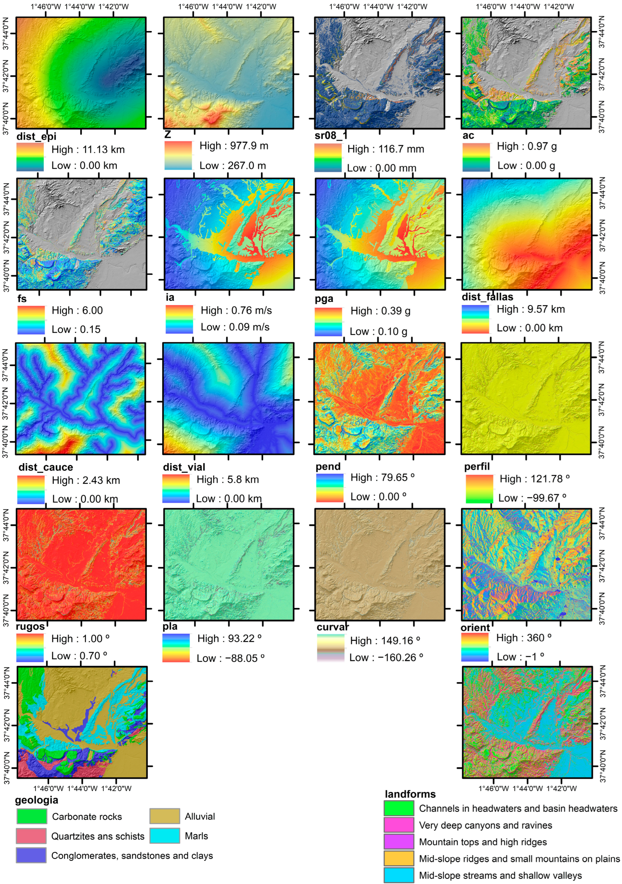
In this study, the existing landslide inventories were merged. This resulted in a total of 257 slope instabilities with different volumes, ranging from one to hundreds of cubic meters. Each mapped slope instability was used to obtain relevant information for landslide control. The parameters used to control the landslide occurrence are shown in

Table 1. Summary of control parameters used in the machine learning methods, classified by the type of information provided and according to their nature.

Type of Information	Slide Control Parameter	Variable	Variable Type
Terrain	Lithology	geologia	Carbonate rocks; quartzites and schists; conglomerates, sandstones, and clays; marls; alluvials
	Morphology	landform	Very deep canyons and ravines; mountain tops and high ridges; u-shaped valleys, flats, open slopes, high slopes, and plateaus; mid-slope streams and shallow valleys; channels in headwaters and basin headwaters; mid-slope ridges and small mountains on plains
	Slope	pend	Continuous quantitative, measured in degrees.
	Slope direction	orient	Continuous quantitative, measured in degrees.
	Concavity/convexity of the terrain	curvar	Continuous quantitative, measured in degrees.
	Concavity/convexity perpendicular to the surface	pla	Continuous quantitative, measured in degrees.
	Concavity/convexity transverse to the surface	perfil	Continuous quantitative, measured in degrees.
	Slope variation in the area occupied by the slope	rugos	Continuous quantitative, measured in degrees.
Location	Distance from slope to the nearest fault plane	dist_falla	Continuous quantitative, measured in km.
	Distance from slope to the nearest transport route	dist_vial	Continuous quantitative, measured in km.
	Distance from slope to the nearest water channel	dist_cauce	Continuous quantitative, measured in km.
	Distance from slope to the epicenter	dist_epi	Continuous quantitative, measured in km.
	Altitude above sea level	z	Continuous quantitative, measured in m.
Earthquake	Newmark displacement	sr08_1	Newmark displacement by [30] measured in cm.
	Critical acceleration	ac	Continuous quantitative, measured in g units (1 g = 9.81 m/s2).
	Safety factor	fs	Continuous quantitative, dimensionless.
	Arias Intensity	ia	Continuous quantitative, measured in m/s.
	Peak Ground Acceleration	pga	Continuous quantitative, measured in g units (1 g = 9.81 m/s2).

and Figure 2. They are grouped into eighteen factors, which provide information about the terrain, location, and seismic parameters that contributed to the landslide triggering.

Factors can be classified into two main categories: categorical and numerical variables. Categorical variables are used to represent different categories or groups of values, whereas numerical variables are used to quantitatively measure a property, either in a discrete or continuous form. Categorical variables represent qualitative information, such as lithology or terrain morphology, whereas numerical variables provide quantitative information, such as slope or roughness.

It should be noted that some dummy variables were included as categorical variables. These variables are represented by binary numeric values, typically 0 and 1, and are used to encode categorical features in machine learning models. By converting a categorical variable into multiple dummy variables, a numerical representation that indicates the presence or absence of a specific category is created. Dummy variables are particularly useful in classification and regression algorithms where categorical features can have a significant impact on data prediction and analysis.

3.1.1. Parameters Related to the Terrain

Lithological units significantly influence the location of landslide phenomena [31], and lithological characterization is one of the most relevant aspects in compiling an inventory of terrain-associated control parameters. The lithological units used in the study were obtained from the geological mapping carried out by the Spanish Geological Survey [32].

Other parameters in the control of landslide triggering include geomorphological factors, such as terrain morphology, slope, curvature, and roughness (Table 1).

Information about the overall curvature of the terrain in a specific direction is obtained using three measures of curvature as follows: total, perpendicular, and transverse concavity/convexity. The total concavity/convexity helps identify areas prone to landslides. Perpendicular concavity/convexity describes the curvature in relation to a vertical line, helping to understand how local terrain features influence slope stability. Transverse concavity/convexity refers to the lateral curvature, allowing the evaluation of how terrain geometry affects the propagation and direction of landslides.

Roughness in landslide analysis refers to variations in the slope. It provides key information about local topographic characteristics and how changes in the slope can affect slope stability and its propagation. Areas with higher roughness tend to have irregularities in the terrain, which increases the likelihood of landslides. Moreover, roughness can influence the velocity and direction of failures.

It is well known that all of these terrain factors significantly influence the distribution, typology, and mechanisms of slope movements [33]. Therefore, they were incorporated into the actual study using several parameters derived from the combined use of the ArcGIS software with the digital elevation model from the Spanish Geographic Institute [34].

3.1.2. Parameters Associated with the Slope Instability Location

Some control parameters are related to the distances of the landslides to the rivers or the nearest roads [35,36]. These parameters provide information about the position of the instability with respect to the environment in which it is located. The distance to the nearest active fault, as well as the distance to the epicenter, are variables that are usually included in landslide susceptibility studies [37,38]. They provide information on the proximity of the slope area to the earthquake location. These parameters can also influence the size and extent of landslides: the closer the area is to the epicenter and the faults, the more likely it is that larger and more extensive landslides can occur. Another parameter with information about the location widely used is the elevation above sea level [35,36,39]. All of these factors were obtained using ArcGIS, based on cartographic databases from the Spanish Geographic Institute [34].

3.1.3. Parameters Related to the Seismic Event

These control parameters provide relevant information about the properties of the seismic event related to the landslide occurrence, such as the peak ground acceleration (PGA) and Arias intensity (I_A). Other parameters that characterize landslide occurrence include the safety factor, critical acceleration, and Newmark displacement. The safety factor (FS) is a parameter used to evaluate the stability of slopes and determine if they are unstable (FS < 1) or not (FS > 1). In this study, FS was calculated using Jibson’s proposal [40], considering the friction angle, cohesion, slope, unit weight, and depth of the sliding block. Critical acceleration is a parameter used in seismic stability analyses and represents the minimum seismic acceleration required to overcome the maximum strength of the slope material and trigger a landslide. The Newmark displacement (D_N) quantifies the expected displacement of a slope during a seismic event, considering different seismic parameters (PGA or I_A) and the distance to the seismic source. The susceptibility to seismically induced landslides is based on the computed Newmark displacement. According to the criteria set by the authors in [41], areas can be divided into non-susceptible (D_N < 1 cm), low susceptibility (D_N = 1–5 cm), moderate susceptibility (D_N = 5–15 cm), and high susceptibility (D_N > 15 cm). All these seismic parameters related to the 2011 Lorca seismic event correspond to those obtained by [27].

3.2. Preparation of Training and Testing Datasets

The total working dataset comprised 6212 sample points, which included both stable and unstable locations (Figure 3). A set of 3106 unstable sites was obtained from pixels within each of the 257 landslides, with an average of 12 to 13 points sampled per instability area. Additionally, a set of 3106 random samples was generated in areas where seismic-induced landslides did not occur with the aim of balancing the dataset. This entire process was carried out using ArcGIS with a pixel size of 5 m. The total working dataset was subsequently split into a training dataset and a testing dataset to train and verify the models, respectively. A random split is performed by assigning 70% of the data to the training dataset and the remaining 30% to the testing dataset.

3.3. Selection of Predictors

Once the training dataset was prepared, relevant variables were selected, i.e., those that have a true relationship with the output to be predicted. The use of too many variables would add noise to the models. Among the different existing variable selection methods, the wrapper methods were used. These methods search for a subset within the dataset that determines the optimal combination of variables, which allows for the best possible performance in predicting the target variable [42].

This present study incorporates variable selection algorithms based on the use of random forests, bootstrap averaging, decision trees, and gradient boosting. In particular, the following methods were used: (i) stepwise forward and backward selection, (ii) Boruta selection model, (iii) recursive feature elimination, (iv) simulated annealing, and (v) genetic algorithms.

Machine learning methods based on decision trees were first described in [43]. These methods learn from the number of times an event occurs compared to another, without considering the order of occurrence of these events. The results are shown in the form of a probability tree. These algorithms are widely used in machine learning techniques, particularly in variable pre-selection, as they have low predictive potential but a high capacity for searching for rules and interactions between variables, particularly categorical variables (since they trace nonlinear relationships very well). One advantage of these pre-selection methods is that they do not assume any theory about the data and properly and efficiently handle the missing data [44]. In addition, decision trees are the basis of other algorithms that have predictive capability, such as bagging, random forest, and gradient boosting.

The precursor of the technique called bagging [45] uses the advantages of decision trees to avoid their predictive instability, thus creating a variable selection technique called bootstrap averaging. It is based on generating multiple versions of a predictor to obtain an aggregated version, which is used to predict the variable and is the starting point in the next step. It obtains a decrease in variance based on the average of previous estimates.

Gradient boosting, proposed by the authors in [46], is based on updating the decrease direction given by the negative gradient of the error function. These algorithms are extremely versatile and are easy to implement and monitor. They have a high predictive capacity and are robust against irrelevant variables, but they are not suitable for problems with low complexity [44].

Among the variable selection algorithms used in this study, stepwise selection methods are based on variable selection using stepwise regression. This method is a hybrid between forward and backward stepwise selections [47]. Forward stepwise selection starts with a model that does not contain any variable, known as the null model. Then, it begins to add significant variables in terms of p-value or lower values in the RSS (residual sum of squares) model sequentially until a specified stopping rule is reached or until all considered variables are included in the model. The stopping rule is usually defined based on a certain p-value threshold, and if the threshold is exceeded, the variable is added to the model. The p-value sensitivity threshold can be defined either fixedly or using AIC (Akaike information criterion) or BIC (Bayesian information criterion). The problem with defining the threshold following these criteria is that the threshold changes for each variable. Backward stepwise selection begins with a full model of variables, which are removed one by one based on a stopping criterion [48]. This selection method allows variables to be selected following a simple and easily interpretable statistical model. However, variable selection is unstable, with a small sample size compared to the number of variables to be studied, as many combinations of variables can fit the data similarly. Additionally, this method does not consider the possible causal relationships between the variables.

The Boruta variable selection model was proposed in [49], which works as an algorithm surrounding Random Forest. This algorithm begins by adding randomness to the dataset. This creates shadow variables from the study variables, which are copied and permuted with each other. Afterwards, a random forest classifier acts on the dataset, where the relative importance of each of the variables is calculated. To evaluate this importance, the decrease in the average accuracy value (mean decrease accuracy) of each feature is used. A greater number of average accuracy values indicates more importance in the model. In each of the iterations, a feature is checked and compared to the importance of its shadow variables. If it is lower than its shadow counterparts, the feature is removed because it is considered to have little importance. This process ends when all the features are confirmed or rejected, or a limit of random forest execution is reached. This variable selection method is relevant because it selects variables that are important to the target variable.

The recursive feature elimination method proposed in [50] is a backward feature selection method, which begins by building a model on the entire set of predictors and calculating the importance order of each predictor. The lowest-importance variables are eliminated, and the model is rebuilt by calculating the importance order of the remaining variables. Backward selection is frequently used with random forest models, as it tends not to exclude variables from the prediction equation and forces the trees to contain suboptimal divisions of the predictors using a random sample of predictors.

Simulated annealing is a method that begins by randomly selecting a subset of entities and defining the operator with a maximum number of iterations. Afterwards, this method builds a model and calculates its predictive performance. Once calculated, it proceeds to include or exclude a small number of features randomly (from one to five) to recalculate the performance and check if it improves or not with the new modification. In the case of worsening, the solution can even be accepted, according to [51], although the acceptance probability decreases as the iteration of the algorithm increases.

The genetic algorithm proposed in [52] is inspired by natural selection and biological evolution processes. Its main objective is to find the optimal set of predictor variables that maximizes model performance. It begins with an initial population of solutions, where each solution represents a set of variables. The performance of each solution is then evaluated using a fitness function that measures the quality of the selected variables. Solutions with higher fitness are more likely to be selected for the next generation. After the selection, genetic operators such as reproduction, crossover, and mutation are applied to generate a new population of solutions. Reproduction involves copying the selected solutions directly into the next generation. Crossover combines the characteristics of two solutions by exchanging parts of their chromosomes. Mutation introduces random changes into a solution to explore new possibilities. This process of selection, reproduction, crossover, and mutation is repeated for several generations until a convergence criterion is reached (e.g., a maximum number of iterations or insignificant improvement in the fitness of the solutions). The final solution obtained represents the optimal set of predictor variables for a given problem.

3.4. Machine Learning Models

The automatic machine learning models used in this study were developed in R software using the auxiliary set of training functions—representation, classification, and regression models from the Caret package (version 6.0-90) created by the authors in [53].

3.4.1. Logistic Regression (LG)

As proposed by the authors in [54], LG is one of the most widely used algorithms for creating machine learning models due to its simplicity. The use of LG falls within the set of generalized linear models and is considered an extension of the linear model. The one-dimensional logistic regression can only correlate the probability of a binary qualitative variable with a scalar variable, thus making its application impossible in the case of multiple predictors. LG can be used with both categorical and continuous variables as the input data. The main limitation of this model lies in its tendency to perform better when the input data are linearly separable, and it is not as effective when there is a nonlinear relationship between the predictor variables and the target variable [55].

3.4.2. Random Forest (RF)

As proposed in [45], as a modification of bagging, RF is based on the incorporation of the randomness of the variables used in the segmentation of each node from the characteristics of the subgroups. Its main attraction is its high generalization capacity and high accuracy rate in problems with a multitude of explanatory variables. This is obtained due to a dimensionality reduction performed internally by the algorithm, reducing any possible overfitting that might arise. This algorithm is suitable for working with both categorical and numerical variables. Its main disadvantage is the high difficulty of interpretation or malfunction in the presence of a low amount of data. It also requires a high number of computational resources to perform the necessary training tasks that guarantee adequate and precise results. Another limitation is associated with difficulties in modeling complex relationships between variables if the number of trees in the forest is not sufficient. Additionally, it can also suffer from overfitting when trained with small or noisy datasets [56].

3.4.3. Artificial Neural Network (ANN)

The current ANN algorithms are based on the backpropagation neuron proposed in [57], i.e., on the mathematical formulation of the averaged backpropagation multilayer neuron. The ANN demonstrated its usefulness in the evaluation of landslide susceptibility phenomena, and its predictive capacity was compared with other algorithms [23,24].

ANN has a high resilient power and fault tolerance, although it is incapable of interpreting learning. The latter is supposed to be a limiting factor since understanding the operation is necessary to validate its prediction in certain fields (e.g., the banking sector).

Among the wide variety of ANNs, feed-forward networks were used in this study, particularly following a model-averaged neural network (avNNet) [58,59]. The idea behind avNNet is to train multiple neural network models with different configurations or initializations, and then average their predictions to obtain a more robust and accurate final prediction. Each individual model can have different architectures or hyperparameters (e.g., number of hidden layers, neurons, and iterations/epochs), allowing for the exploration of different approaches and avoiding reliance on a single model. Averaging the models helps to reduce overfitting and improves the generalization ability of the final model. By combining the predictions of multiple models, the impact of individual decisions is diminished, leading to a more reliable consensus.

The stopping criterion plays a crucial role in ANN performance: it indicates when to stop the training process. In this study, cross-validation was used as the stopping criterion [60]. This technique involves dividing the data into training and validation sets and then evaluating the model’s performance on the validation set at each stage of training. To do this, the loss and val-loss curves are plotted throughout different training epochs. As these curves descend, the model correctly generalizes. The training process stops when the loss curves start to increase because the following epochs cause an overfitting of the model.

It is also important to perform a sensitivity analysis to assess the robustness and influence of the different variables on the model’s response. In binary classification, an accuracy metric can be used to evaluate different sets of predictors. This allows for examining how the model’s accuracy varies when modifying the feature sets or input variables.

ANNs are flexible and can work with various types of data, such as images, text, and numerical data. Their main limitation is the need for large amounts of data to train effectively, especially when dealing with deep architectures. Additionally, their complexity and the need to adjust multiple hyperparameters can make their implementation and optimization challenging [61].

3.4.4. Support Vector Machine (SVM)

SVM is a set of algorithms that emerged in the early sixties [62] and is focused on the linear separation of classes using algebraic methods. Their objective is to find a hyperplane that linearly separates a binary distribution in the best possible way. Its applicability is not only limited to monoclass problems, as in the case of seismically induced landslides [25,26], but it can also be used to solve multiclass problems [63] resorting to a binary reduction.

The foundation of SVM models is based on the transformation of characteristics using kernel functions (linear, polynomial, and sigmoidal) [64,65], which assign the data to a different dimensional space to separate the classes more easily. Thus, it simplifies the nonlinear decision bounds to linear bounds in the eigenspace.

SVMs can be used with numerical or numerically encoded categorical data. Their limitations depend on the kernel being used. In the case of a linear kernel, these algorithms are not suitable for nonlinear classifications and may struggle when the data are highly overlapping or when there are multiple overlapping classes. In the case of the radial kernel, they are highly sensitive to the selection of hyperparameters, such as the kernel width. Additionally, SVMs can be computationally expensive to train on very large datasets [66].

3.4.5. Model’s Differences

The LG is a linear classification model that estimates the probability of belonging to a particular class. Unlike the other mentioned models, LG assumes a linear relationship between the predictor variables and the target variable. However, this limits its ability to capture nonlinear patterns in the data. In contrast, RF is an ensemble of decision trees that combines the individual predictions of each tree to obtain a final prediction. Unlike LG, RF can capture nonlinear relationships and perform well on complex datasets. ANNs are highly flexible and powerful models that consist of interconnected layers of nodes. Unlike the previous models, ANN can learn complex nonlinear representations of the data, enabling them to adapt to a wide range of problems. As for the SVM, they come in two variants: a linear kernel and a radial kernel. The SVM with a linear kernel (SVML) uses a linear function to map the data to a higher-dimensional space, whereas the SVM with a radial kernel (SVMR) uses a nonlinear function that allows for classification in more complex feature spaces.

In summary, the differences between all these models lie in their ability to capture nonlinear relationships, the flexibility in data representation, and the complexity of the problems to address. While LG is limited to linear relationships, RF and ANN are better suited for nonlinear relationships. Within SVMs, a linear kernel is used in cases of linear separation, whereas a radial kernel is more flexible and can address more complex problems.

3.5. Model Evaluation

The evaluation of the models entailed two differentiated phases. The first phase consisted of an evaluation of the statistical results by machine learning models using a subset of 1864 test slides, which comprised 30% of the total dataset. To evaluate the performance of the developed classification models, different metrics were employed as follows: the confusion matrix, classification error rate, area under the curve, and combined performance.

The confusion matrix shows the number of times the model correctly or incorrectly predicted each of the classes in the classification problem. It has four main elements: true positives (TP), false positives (FP), true negatives (TN), and false negatives (FN).

The classification error rate or classification error (error) is a metric used to evaluate the performance of a classification model. It is defined as the proportion of incorrect predictions made by the model relative to the total number of predictions made. A high classification error rate indicates that the model struggles to correctly classify the samples into their respective classes. This suggests that the model may not be suitable for a given dataset. The error rate can be calculated using Equation (1):

$$\mathrm{Error}=\frac{\mathrm{FP}+\mathrm{FN}}{\mathrm{TP}+\mathrm{TN}+\mathrm{FP}+\mathrm{FN}}$$

(1)

The area under the curve (AUC) is a metric used to evaluate the performance of binary classification models. AUC refers to the area under the receiver operating characteristic (ROC) curve, which is a graphical representation of the relationship between the true positive rate (TPR, Equation (2)) and the false positive rate (FPR, Equation (3)) across different decision thresholds.

$$\mathrm{TPR}=\frac{\mathrm{TP}}{\mathrm{TP}+\mathrm{FN}}$$

(2)

$$\mathrm{FPR}=\frac{\mathrm{FP}}{\mathrm{TN}+\mathrm{FP}}$$

(3)

The AUC ranges from 0 to 1: a value of 1 indicates the perfect ability of the model to distinguish between classes; a value of 0.5 indicates random performance. The AUC provides a balanced assessment of the model’s performance by considering its ability to distinguish between both classes.

The combined performance (PC) combines two model evaluation metrics: the classification error rate and AUC. This can be calculated using Equation (4):

$$\mathrm{PC}=\left(1-\overline{\mathrm{Error}}\right)\ast \overline{\mathrm{AUC}}$$

(4)

where $\overline{\mathrm{Error}}$ corresponds to the average error rate of all classes, and $\overline{\mathrm{AUC}}$ refers to the average area under the ROC curve for all obtained classes. This approach provides an overall evaluation of the model’s performance that considers both its ability to distinguish between classes and its accuracy in classifying each class. By combining these two metrics, a more comprehensive assessment of performance can be obtained.

It should be noted that in the definition of PC, both the error and AUC evaluate binary classification models, but they are not necessarily equally important. The error is a more critical measure for evaluating the model; it indicates how well the model is classifying observations into the correct categories. The AUC measures the model’s ability to distinguish between the two classes, but it does not necessarily indicate how well observations are classified into the correct categories. In this study, both measures were considered equally significant, so equal weights were assigned.

To improve the generalization ability of the models and select the best parameters, repeated cross-validation was applied. This was performed using the ‘trainControl’ function implemented in Caret as a common training control parameter. The purpose of this cross-validation was to repeat the process a total of five times for each model to obtain a more accurate estimate of the model performance. A total of 10 folds were specified to be used in cross-validation for each repetition of the model. At the same time, a hyperparameter grid was implemented for each model during the cross-validation training phase. This was possible by using Caret’s ‘expand.grid’ function, which created all possible combinations of the selected parameter values.

In the case of LG models, no hyperparameter grid was used. In such cases, only repeated cross-validation was implemented in the training phases of each of the six different LG models, using the number of epochs defined in the general cross-validation function as the stopping criterion. Each model was trained and validated 50 times (10 times in each repetition of cross-validation) during the entire training and validation process.

For the RF models, a different hyperparameter grid was implemented for each model, along with repeated cross-validation. The parameter adjusted was ‘mtry’, i.e., the number of variables selected for each partition of each tree in the forest. The maximum value set for each model corresponded to the integer nearest to the square root of the number of variables considered. The minimum value used was 1 and the rate of variation between the maximum and minimum values was also 1. To develop each of the models, a depth of 300 trees was established for each RF, with a minimum of ten observations per tree leaf with replacement.

In the case of the ANN models, a network architecture was implemented using the average of the created models (avNNet) with a maximum number of 145 iterations. This architecture is not a specific or optimal architecture for the case study, but its success primarily depends on the number of analyzed parameters [67]. In each of the ANN, a different hyperparameter grid was implemented, as well as repeated cross-validation. The adjusted hyperparameters corresponded to the ‘size’ parameter or neurons in the hidden layer of the network. The maximum value set in each model for this parameter corresponded to the maximum number of variables in each of the sets. The minimum value was taken as 1. The rate of variation between the maximum and minimum used was also 1. In addition, the hyperparameter ‘decay’ or L2 penalty rate was also applied to the weights of the network. The explored penalty values were 0.1, 0.01, and 0.001. To avoid increasing the model’s bias, the use of replacement sampling was disabled in each model.

The models created using SVM with a linear kernel (SVML) were constructed by employing a different hyperparameter grid in addition to repeated cross-validation. The hyperparameter corresponded to the regularization parameter ‘C’, which controlled the trade-off between classification accuracy and model complexity. This parameter was tuned in two rounds. In the first round, different standard values of C (0.01, 0.05, 0.1, 0.2, 0.5, 1, 2, 5, and 10) were tested to select a range of values, to be later expanded in a second round, and to select the regularization value that resulted in a balance between the margin of error and higher model accuracy.

In the case of SVM with a radial basis function kernel (SVMR), they were also created with a different hyperparameter grid in each model, in addition to repeated cross-validation. The hyperparameters to be adjusted were two: the regularization hyperparameter of SVMR and the ‘sigma’ hyperparameter or radial kernel bandwidth in the model. These two hyperparameters were adjusted in two rounds, where the kernel bandwidth hyperparameter was tested with different standard values (sigma: 0.0001, 0.005, 0.01, 0.05, 0.1, 1, 10, and 100).

To complete this phase of validation, the models that use the dataset provided by the principal component analysis were also developed in the same way as their counterparts. Principal component analysis (PCA) is a statistical method aimed at reducing the dimensionality of data. Its objective is to obtain a new set of uncorrelated variables called “principal components”, which capture the most information in terms of the variance of the original data. This technique is widely used in various fields [68] to perform tasks such as dimensionality reduction, data visualization, pattern detection, and exploration of the underlying structure in a set of variables.

3.6. Validation and Comparison with Physical Methodologies

The next phase of validation (starting from the qualification of the statistical models in the previous section) was aimed at verifying that the models with the best scores had the same or similar successes as those obtained in the predictions using the physical methodology [27,69]. Starting from the hazard maps in terms of probability 0–1, a common probability threshold (70%) was established for all the models. This enabled discrimination in unstable areas from those that were not. This value was used to obtain the total area covered (TAC) and the ground failure capture (GFC). The total area covered (TAC) represents the percentage of the area predicted to be prone to landslides in relation to the total area, while the ground failure capture (GFC) expresses the actual percentage of landslides within the area predicted by TAC. The difference between GFC and TAC is a combined indicator that reflects the accuracy of the model’s predictions. Higher values of this difference indicate more accurate predictions, as the predicted extent is smaller compared to the actual number of landslides. On the contrary, lower values of this difference suggest poorer predictions, as a larger extent prone to landslides is forecasted than what occurs. The coefficient used for the final validation was the success rate (SR) corresponding to the multiplication of GFC by the difference between GFC and TAC. The greater the amount of SR, the greater the coherence and accuracy between the prediction and the real position of the slope instabilities according to the actual inventory.

4. Results

4.1. Slope Instability Control Parameters

The analysis of the starting data showed that the seismic-induced landslides were mainly triggered by clayey and carbonate materials, whose average slope value was 31°. Half of these seismic-induced landslides were found 2.79 km from the fault plane and 3.72 km from the epicenter of the earthquake. These landslides were located on average 1.50 km away from the roads and 500 m from the rivers and at an average elevation of 493 m.

4.2. Preparation of the Training Dataset

One of the categorical variables studied exhibited a distribution in poorly fitting classes. As a result, the variable “landform” was binarized and recategorized, combining three classes into one group coded as “landform.grouped”. This new category included the classes labeled “Mid-slope channels and few deep valleys”, “Channels in the headwaters and headwaters of the basins”, and “Crests on the middle slopes and small mountains in the plains”. In the same way, the continuous variable of the Newmark displacement (D_N) was chosen and grouped into three displacement intervals (D_N < 1; D_N = 1–15; D_N > 15) to reduce the high number of outliers in the variable. After cleaning and normalizing the data, a total of 15 new dummy variables were created from the categorical variables, resulting in a total of 30 variables. In contrast, a high correlation was observed between several variables, with covariance values greater than 75%. Variables that exceeded 70% correlation were decided to be excluded, which is common in statistics. Removed variables were the distance from slope to the nearest road (distancia_vial), distance from slope to the epicenter (dist_epi), total concavity/convexity (curvar), safety factor (fs), altitude (z), and the dummy variable “landform.grouped”.

The transformation of the data into new principal components can be seen in

Table 2. Coefficients resulting from the reduction in dimensionality by principal components.

VARIABLE	CP1	CP2	CP3	CP4	CP5	CP6	CP7	CP8	CP9	CP10	CP11	CP12	CP13	CP14
Dist_falla	0.0872	0.2976	0.0588	−0.3687	−0.0365	−0.0459	−0.0341	−0.0686	−0.0008	−0.0308	0.0285	0.2105	0.0899	0.0899
Dist_vial	0.3221	0.0767	0.0109	0.2089	0.0779	−0.0904	−0.0832	−0.0730	−0.0112	−0.0606	0.0650	0.1817	0.0432	0.0432
Dist_cauce	0.2355	0.0052	0.0052	0.2591	0.1566	0.0071	0.0417	0.0106	0.0500	0.0374	−0.1028	−0.0654	−0.0252	−0.0252
Dist_epi	0.1695	0.3363	0.0645	−0.3274	0.0860	−0.0166	−0.0131	−0.0101	0.0500	−0.0249	−0.1035	0.0356	0.0730	0.0730
Pend	0.2093	−0.3335	−0.0885	−0.0604	0.1735	0.0713	0.0780	−0.0657	0.0400	−0.0676	−0.0328	0.0753	−0.0794	−0.0794
Orient	0.0127	−0.0383	0.0063	0.0342	−0.1341	−0.0321	0.1938	0.0883	0.0892	0.2370	0.4777	0.7242	0.1160	0.1160
Curvar	0.0085	−0.1065	0.5291	0.0077	−0.0211	0.0361	−0.0289	−0.0091	0.0017	−0.0221	−0.0320	0.0125	0.0280	0.0280
Pla	0.0156	−0.1128	0.4045	0.0041	0.0078	0.0504	0.0027	0.0402	0.0151	−0.0219	0.0528	−0.0489	0.0903	0.0903
Perfil	−0.0038	0.0764	−0.4890	−0.0111	0.0346	−0.0189	0.0463	0.0383	0.0179	0.0211	0.0772	−0.0516	0.0263	0.0263
Rugos	−0.0451	0.2800	−0.0311	0.1656	0.0246	0.5264	−0.0094	−0.0058	0.0335	−0.0422	−0.0539	0.0461	−0.0726	−0.0726
Ac	0.2098	0.0217	0.0067	0.0831	−0.4915	−0.0650	0.0187	0.1542	−0.0884	0.0422	0.1429	−0.2892	0.0159	0.0159
Fs	−0.3026	−0.1868	−0.0221	0.2561	0.0330	−0.0403	0.0416	−0.0312	−0.0367	0.0274	0.1300	0.0293	−0.0707	−0.0707
Ia	−0.2925	−0.2277	−0.0377	0.3297	0.0213	−0.0164	0.0314	−0.0185	−0.0258	0.0244	0.0809	−0.0121	−0.0627	−0.0627
Pga	0.3817	0.0089	0.0082	0.1792	0.1276	−0.0491	−0.0043	−0.0545	0.0116	−0.0157	0.0141	0.0732	−0.0205	−0.0205
Z	0.3817	0.0089	0.0082	0.1792	0.1276	−0.0491	−0.0043	−0.0545	0.0116	−0.0157	0.0141	0.0732	−0.0205	−0.0205
Geology.Carbonates_rocks	0.1454	−0.005	0.0383	−0.2081	0.1567	0.0984	0.3043	0.1710	−0.0300	0.4773	0.2463	−0.2799	−0.3916	−0.3916
Geology.Quartzites_and_schists	0.1769	0.0217	−0.0179	0.2209	0.1147	−0.0569	−0.4593	−0.2682	−0.2043	−0.0939	0.2398	−0.0960	0.0775	0.0775
Geology.Conglomerates, sandstones_and_clays	0.1076	−0.0075	−0.0194	0.2592	−0.1609	−0.1218	0.3519	0.2830	0.3296	−0.1395	−0.4705	0.0996	0.1655	0.1655
Geology.Marls	−0.0505	−0.2189	−0.0658	−0.2475	−0.4190	0.1406	−0.2045	−0.0314	−0.0922	−0.2111	0.0101	0.0782	0.1655	0.1655
Geology.Alluvial	−0.2908	0.1986	0.0593	0.0294	0.3044	−0.0727	0.0139	−0.1300	0.0058	−0.0108	−0.0213	0.1496	−0.0214	−0.0214
Landform.Very_deep_canyons_and_ravines	0.0145	−0.0771	−0.3547	−0.1163	−0.0093	−0.4778	0.0146	−0.0683	−0.1555	0.0524	−0.1141	0.0327	−0.0472	−0.0472
Landform.Mountain_tops_and_high_ridges	0.0460	−0.2445	0.3485	−0.1180	0.0496	−0.3213	0.0293	−0.0795	0.0523	0.0322	−0.0024	−0.0495	−0.0019	−0.0019
Landform.U-shaped_valleys	0.0242	0.0159	−0.0563	0.0371	−0.1702	0.1119	−0.4580	0.0821	0.6435	0.0843	0.0770	0.0271	−0.3377	−0.3377
Landform.Flats	−0.2456	0.1903	0.0539	0.0040	0.2653	0.0160	−0.0360	0.0317	0.0032	0.0399	−0.1233	0.0146	0.1429	0.1429
Landform.Open_slopes	0.0680	0.1235	0.0180	0.1125	−0.2896	0.2842	0.4090	−0.5021	−0.1990	−0.1074	0.0010	0.0107	−0.1348	−0.1348
Landform.High_slopes_and_plateaus	0.0722	−0.0202	−0.0006	0.0647	0.1106	0.2236	−0.1586	0.6314	−0.4866	−0.0188	−0.0368	0.1286	0.0745	0.0745
Landform. grouped	0.0364	−0.0569	−0.1061	−0.0351	0.1798	0.1332	0.1849	0.0223	0.2940	−0.1069	0.4052	−0.3380	0.6357	0.6357
Sr08_1 less_than_1	−0.1034	0.3755	0.1115	0.1698	−0.1450	−0.2778	0.0308	0.1203	−0.0319	−0.0945	0.19997	−0.1061	−0.0493	−0.0493
Sr08_1 from_1_to_15	0.0431	−0.1075	−0.0380	0.0551	−0.0907	0.1473	−0.1656	−0.2140	−0.0383	0.7011	−0.3217	0.0192	0.3672	0.3672
Sr08_1 greater_than_or_equal_to_15	0.0870	−0.3439	−0.0987	−0.2145	0.2080	0.2158	0.0609	−0.0080	0.0561	−0.2968	−0.0325	0.1035	−0.1556	−0.1556

. This was carried out by condensing the information into 14 new variables, which explained 87.37% of the total variance. These new principal components called “CP_” allowed for obtaining the new values of the 14 components, using the application of the coefficients that multiply the value stored in the original data.

4.3. Selection of Predictors

A total of six sets of predictors were created, five of which came from the application of different selection models, and one considered all the variables (

Table 3. Predictor distribution for each of the six sets established in the study.

VARIABLE	SET-1	SET-2	SET-3	SET-4	SET-5	SET-6
Dist_falla	X	X	X	X	X	X
Dist_vial						X
Dist_cauce	X		X		X	X
Dist_epi						X
Pend	X	X	X	X	X	X
Orient		X	X	X	X	X
Curvar						X
Pla				X		X
Perfil	X	X	X	X		X
Rugos	X	X	X		X	X
Ac			X			X
Fs						X
Ia	X	X	X	X	X	X
Pga	X	X	X	X	X	X
Z						X
Geology.Carbonates_rocks			X			X
Geology.Quartzites_and_schists			X			X
Geology.Conglomerates, sandstones_and_clays		X	X	X	X	X
Geology.Marls		X	X	X		X
Geology.Alluvial		X	X	X	X	X
Landform.Very_deep_canyons_and_ravines		X		X	X	X
Landform.Mountain_tops_and_high_ridges			X		X	X
Landform.U-shaped_valleys		X		X	X	X
Landform.Flats		X		X	X	X
Landform.Open_slopes		X	X	X	X	X
Landform.High_slopes_and_plateaus		X		X	X	X
Landform. grouped						X
Sr08_1. less_than_1		X	X	X	X	X
Sr08_1. from_1_to_15		X		X	X	X
Sr08_1 greater_than_or_equal_to_15			X			X

). The first set (SET-1) was made from random forests (Boruta model) resulting in a selection of seven variables. The second set (SET-2) was prepared using the stepwise forward and backward selection method, resulting in a selection of 17 variables. The third set (SET-3) was elaborated from the recursive elimination of variables, resulting in a selection of 18 variables. The fourth set (SET-4) was made from simulated annealing, resulting in a selection of 17 variables. The fifth set (SET-5) was elaborated from the application of the genetic algorithm, resulting in a selection of 17 variables. The last set (SET-6) included all the variables.

Additionally, a single set corresponding to the 14 variables created previously in the PCA (Table 2) was also used (SET-CP).

4.4. Models and Statistical Validation

The machine learning models were trained independently using each of the six sets of predictors individually.

Figure 4 shows a comparison of the different LG models with the training data. To establish the best model, both the error and AUC of each model were needed for analysis. This information is also provided in

Table 4. Combined performance value for each LG model built from each set of developed predictors.

Predictor	Average AUC (%)	Average Error Rate (%)	Combined Performance (%)
SET-1	92.20	14.86	78.50
SET-2	94.19	12.74	82.19
SET-3	94.03	13.27	81.56
SET-4	87.97	20.76	69.71
SET-5	94.16	12.91	82.00
SET-6	94.02	13.08	81.73

, along with the combined performance. Both criteria are consistent since combined performance is a combination of model accuracy and discrimination ability (represented by AUC), whereas error and AUC are independent measures. A model can have a high AUC and a high error rate, which means it has good discrimination ability but may misclassify some instances. Similarly, a model can have a low AUC and a low error rate, which means it has high accuracy but low discrimination ability. Therefore, a model with a low error and high AUC is considered better than the others. According to these criteria, all SETs are good in terms of AUC and error rate (above 94% and below 14%, respectively), apart from SET-1 and SET-4, which experience a decrease in such scores. The model using the predictor SET-2 shows the lowest average error (12.74%) and the highest average AUC (94.19%), being the best model. It is important to note that, although the model using the variables selected via the genetic algorithm (SET-5) has the second-best performance in terms of AUC (94.16%), its performance in terms of error is considerably inferior to that of the selected model (12.91%). Combined performance results also show the same trend, with SET-2 as the model that has the highest performance rate value (82.19%).

Figure 5 compares the best RF model already adjusted based on the ‘mtry’ parameter to the training data. In general, all the models achieve a good score in terms of combined performance (above 84%), except for SET-4 (

Table 5. Combined performance value for each RF model built from each set of developed predictors.

Predictor	Average AUC (%)	Average Error Rate (%)	Combined Performance (%)
SET-1	95.08	11.30	84.33
SET-2	95.11	11.10	84.56
SET-3	95.31	10.89	84.94
SET-4	92.57	14.24	79.39
SET-5	95.25	10.97	84.80
SET-6	95.08	11.16	84.47

). This behavior may reflect that the parameter combination adopted by the corresponding predictors does not work as well as the other combinations analyzed with different predictor sets. Under the criteria of high AUC and low error, the best model corresponds to SET-3, with ‘mtry’ value of 4. This model achieved 95.31% AUC and a 10.89% error rate (Table 5). Under the criteria of combined performance, the best model is also SET-3, as it has the highest value (84.94%), followed by SET-5 and SET-2. This indicates that SET-3 has the most balanced combination of accuracy and discrimination ability, whereas SET-5 and SET-2 have slightly better accuracy than SET-3, but with slightly worse discrimination ability.

Figure 6 shows a comparison of the best-adjusted ANN models. The optimal number of neurons in the hidden layer and the regularization parameter value for each of the models are shown in

Table 6. Optimal hyperparameter values for each of the average ANN models created from the training data.

Predictor	Hidden Nodes	L2 Penalty Rate	Average AUC (%)	Average Error Rate (%)	Combined Performance (%)
SET-1	5	0.10	94.42	11.67	83.39
SET-2	17	0.10	94.87	10.93	84.49
SET-3	9	0.10	95.21	10.27	85.43
SET-4	10	0.01	91.27	15.80	76.85
SET-5	13	0.10	95.00	10.98	84.57
SET-6	10	0.10	94.81	11.01	84.37

. The table shows that all sets reach similar combined performance values (above 83%), except for SET-4, which shows a decrease. The model with the best performance is SET-3 since it has the highest AUC value (95.21%) and the lowest error rate (10.27%). Under the combined performance criterion, the model with the best performance is also SET-3 since it has the highest value (85.43%). Both criteria are coincident, suggesting that it is a robust and reliable model. To ensure the robustness of this model, the loss function was analyzed in comparison to the validation loss (Figure 7). Both metrics decrease as the size of the training set increases. They converge and reach a low value, indicating high model robustness and generalization capability.

Furthermore, the data dispersion does not seem to be large enough to significantly affect the model selection, as there is no great variability in the values for each metric of the analyzed models. This suggests that the results are consistent and are not significantly influenced by outliers or extreme values in the data. Additionally, the average AUC and error values for each model are quite stable and remain within a narrow range of values.

Figure 8 and

Table 7. Optimal hyperparameter values for each of the SVML models created from the training data and combined performance metric.

Predictor	Regularization Parameter	Average AUC (%)	Average Error Rate (%)	Combined Performance (%)
SET-1	0.03	92.17	14.86	78.47
SET-2	0.44	94.11	12.71	82.15
SET-3	1.88	94.03	13.16	81.66
SET-4	0.003	87.86	20.55	69.81
SET-5	0.50	94.11	12.83	82.03
SET-6	1.09	93.89	13.03	81.66

show the comparison of the different SVML models with the optimal regularization parameter. All sets seem to achieve very good results in the combined performance (above 81%), except for SET-1 and SET-4, which experience a considerable decrease. The model SET-2 was selected with a value of 0.44 in the regularization hyperparameter and has the highest AUC (94.11%) and the lowest error rate (12.71%). The model SET-5 has the same AUC (94.11%), but a slightly higher error rate (12.83%). Analysis of the combined performance shows that the model with the best score is SET-2 (82.15%), followed by SET-5. Since the metrics are very similar, the visual information provided in Figure 8 (distribution of the data) helps in taking decisions, as it leads to identifying the presence of outliers and their dispersion. For SET-5, the AUC boxplot shows a relatively symmetrical distribution, with a median of around 0.94 and moderate data dispersion. The error boxplot shows a left-skewed distribution, with a median close to 0.125 and the presence of outliers. In the case of SET-2, the AUC boxplot shows a distribution similar to that of SET-5, with a median of around 0.94 and moderate data dispersion. The error boxplot shows a left-skewed distribution, with a median close to 0.126, and the presence of outliers like SET-5. Overall, both models present similar distributions in terms of AUC, although SET-5 seems to have a higher concentration of data around the median. Regarding the error, both models present a left-skewed distribution and the presence of outliers. Based on this information, it is difficult to decide with certainty which of the two models is better. Considering only the performance in terms of AUC and error, both models present similar results. However, when the presence of outliers is considered, SET-2 shows a better performance, as it has fewer outliers in the distribution.

Figure 9 shows a comparison of the SVMR models with the optimal regularization parameters presented in

Table 8. Optimal hyperparameter values for each of the SVMR models created from the training data, and combined performance metric.

Predictor	Regularization Parameter	Kernel Bandwidth	Average AUC (%)	Average Error Rate (%)	Combined Performance (%)
SET-1	1.90	0.05	93.83	13.41	81.24
SET-2	1.95	0.05	94.48	12.03	83.11
SET-3	2.00	0.05	94.86	10.56	84.84
SET-4	1.80	0.05	91.17	17.07	75.61
SET-5	2.00	0.05	94.39	11.92	83.14
SET-6	2.00	0.05	94.70	11.72	83.60

. The results follow the same behavior, with all sets reaching very good results in the combined performance (above 83%), except for SET-1 and SET-4. The model that uses predictors from SET-3, obtained via recursive variable elimination, was selected with a regularization hyperparameter value of 2 and a bandwidth hyperparameter value of 0.05. Under the criteria of higher AUC and lower error rate, this model achieved the best score, with an AUC value of 94.86% and an error rate of 10.56%. Under the combined performance criteria, the best model is SET-3, as it has the highest value (84.84%). The second-best model corresponds to the model that uses all the variables (SET-6), with an AUC value of 94.70% and an error rate of 11.72%. Under the combined performance criteria, the model that uses SET-6 remains in second place. Therefore, both criteria coincide with the selection of the first- and second-best models, as the SET-3 model performs better in both performance measures in terms of AUC, error, and combined performance. This decision is further validated by analyzing the boxplot of the models in shown Figure 9. The SET-3 model is observed to have a more concentrated distribution, with values closer to an AUC of 0.95 and an error of around 0.1, while the points representing the SET-6 model are more dispersed, covering a wider range in both AUC and error rates. Therefore, the SET-3 model has less dispersion in both AUC and error than the SET-6 model, indicating that the AUC and error values of the SET-3 models are more consistent and closer to each other.

Table 9. Optimal hyperparameter values for each of the models created using principal components (_cp). The models used correspond to the following: ann, artificial neural networks; lg, logistic regression; rf, random forest; svml, support vector machine with linear model; svmr, support vector machine with radial base model.

Model	Regularization Parameter	Kernel Bandwidth	Hidden Nodes	L2 Penalty Rate
lg_cp	-	-	-	-
rf_cp	4	-	-	-
ann_cp	-	-	10	0.1
svml_cp	4.80	-	-	-
svmr_cp	4.95	0.05	-	-

and

Table 10. Summary of the metrics obtained in the testing and validation phases of the different models, with each of the available sets of predictors. The models used correspond to the following: ann, artificial neural networks; lg, logistic regression; rf, random forest; svml, support vector machine with linear model; svmr, support vector machine with radial base model. In addition, models that use principal components as predictor variables are considered. These models can be identified by the notation “_cp” in the “Model” column.

Model	Predictor	Training			Testing
		Av. AUC	Av. Error	Comb. per.	Av. AUC	Av. Error	Comb. per.
ann	SET_3	0.952	0.103	0.854	0.914	0.110	0.813
ann_cp	--	0.954	0.101	0.858	0.901	0.115	0.797
lg	SET_2	0.942	0.127	0.822	0.879	0.155	0.743
lg_cp	--	0.919	0.155	0.777	0.848	0.160	0.712
rf	SET_3	0.953	0.109	0.849	0.925	0.110	0.823
rf_cp	--	0.953	0.110	0.848	0.892	0.155	0.754
svml	SET_2	0.941	0.127	0.822	0.880	0.155	0.744
svml_cp	--	0.918	0.158	0.773	0.848	0.163	0.710
svmr	SET_3	0.949	0.106	0.848	0.909	0.113	0.806
svmr_cp	--	0.941	0.122	0.827	0.896	0.124	0.785

show the optimized hyperparameter values of the models with principal components and performance metrics, respectively, for the dataset provided by the PCA. The best model according to the criteria of the highest AUC and lowest error rate corresponds to the ANN (ann_cp) since its error rate is 10.10% and its AUC is 95.40%, making it the best model. When the training results are analyzed based on the combined performance criterion, the ANN also shows the highest value in this metric (85.80%). Both metrics show that the ANN using principal components has the highest performance. The second-best model in the training phase is RF (rf_cp), as it has an AUC of 95.31% and an error rate of 11.0%, leading to lower combined performance (84.80%).

5. Discussion

5.1. Performance and Comparison of Selected Models for Landslide Susceptibility Assessment

The best selected models were tested on the test dataset to evaluate their final performances (Table 10). The best model is RF, which uses predictor SET-3 and achieves the highest AUC value (92.50%) and the lowest error rate (11.00%). If the results are analyzed with respect to the combined performance criteria, this model is also the best, with a score of 82.30%. The next best models are ANN and SVMR, both using SET-3, with a combined performance of 81.30% and 80.60%, respectively.

All in all, RF using SET-3 may be selected as the best model. This means that variables that control co-seismic landslides include distance to faults and rivers, slope angle, orientation, roughness, curvature, critical acceleration, Arias intensity, PGA, lithology, Newmark displacement, and landform (mountain tops, high ridges, and open slopes). Good performance of RF was also obtained by the authors in [22] in their global susceptibility assessment study, with a predictive capacity slightly higher (AUC of 98.50%) when compared to the results obtained in this study (AUC of 92.50%). It is important to note that there is an agreement between both studies that the distance to faults and slope angle are important predictive variables for this algorithm.

The second-best model corresponds to the ANN model using an average of the model (avNNet). As in the case of the results obtained by the authors in [23], the most important factors for landslide susceptibility using ANN correspond to profile curvature, topographic moisture index, and slope. Other influential variables related to the distance to roads and rivers have been shown in other studies [24]. In terms of pixel classification, the results obtained using MLP by the other authors and the results of this study are similar, being slightly higher in this study (91.40% AUC), which may indicate that the ANN that uses the an average usually converges better in assigning weights for co-seismic landslide identification.

In the case of SVM models, the best-performing models correspond to the radial basis function kernel (RBF) as opposed to the linear kernel. The former achieved AUC values of 90.90% compared to the latter, which reached an AUC of 84.8%. Comparing the accuracy results with those reported in [26], similar values are observed, but the results in this study are higher. This may be because the present data has a higher degree of nonlinearity. Similarly, it is agreed that the best kernel function for modeling landslide susceptibility data corresponds to the radial function (RBF). When comparing the results with those of [25], there is agreement on the need for good data preparation to avoid biases in predictive models.

Finally, if we compare the results obtained using LG models with those provided in [19], both studies show good results in terms of the ROC curve. The value obtained by these authors was quite high, which could reflect a possible overfitting of the model to the data. In contrast, the results obtained in [20] are more similar to those obtained in this study in terms of the ROC curve. Both authors agree that the most relevant variables for this algorithm are terrain slope, slope orientation, lithology, and PGA.

5.2. Validation and Comparison with Physical Methodologies

Table 11. Summary of the comparison of seismic-induced landslide hazard maps of each statistical model and the actual location of the mapped slope instabilities. The models used correspond to the following: ann, artificial neural networks; lg, logistic regression; rf, random forest; svml, support vector machine with linear model; svmr, support vector machine with radial base model. Models identified by the notation “_cp” correspond to models that use principal components.

Model	% TAC	% GFC	% GFC–% TAC	% SR
ann_cp	19.85	90.27	70.42	63.57
svmr_cp	19.66	89.88	70.22	63.12
lg_cp	19.61	86.38	66.48	57.42
svml_cp	19.65	85.21	65.56	55.87
rf_cp	16.08	81.71	65.63	53.63
svmr	11.53	74.71	63.18	47.20
ann	11.22	74.32	63.10	46.90
svml	13.95	74.32	60.36	44.86
lg	13.81	73.93	60.12	44.45
rf	3.57	39.69	36.12	14.33

displays the percentage values of the TAC, GFC, and SR indicators for the selected best models in statistical terms, which assess their performance regarding the actual location of slope instabilities triggered by the 2011 Lorca earthquake.

Upon analyzing the results provided by the machine learning models, it is observed that the SR coefficient values range from 44% to 47%, except for the RF model, which has the lowest SR score (14.33%). It is worth noting that this model is the best in statistical terms, but it performs the worst in terms of the SR indicator, as its predictions fail to effectively model the co-seismic landslide’s location. On the contrary, SVMR achieves the highest score in terms of the SR indicator (47.20%), despite being the third-best model in statistical terms, followed by the ANN model in terms of SR (46.90%), which is the second-best model in statistical terms. Considering both models, the variables that control the co-seismic landslide occurrence are the same as those explained above for the RF model. These results agree with those of [23], in which curvature was selected as a relevant variable. Additionally, [24] emphasized the distance to rivers, whereas [25] highlighted the importance of proper data preparation to avoid biases in predictive models. This finding supports the relevance of these variables in predicting co-seismic landslides.

When conducting the same analysis with the machine learning models built from principal components, all models show substantial improvement in terms of the SR indicator, with values exceeding 50%. The principal components retain more information in terms of the explained variance of the features, enabling more accurate predictions throughout the entire map. The model corresponding to ANN (ann_cp) achieves the highest score for the SR indicator (63.57%), although it does not suggest being the best statistically among all the analyzed predictive models. According to this model, the variables that control the co-seismic landslide include orientation, Newmark displacement, landform, curvature, roughness, PGA, Arias intensity, and lithology (alluvial). Comparing the variables selected by the PCA with those in SET-3 shows substantial agreement. However, when comparing with those selected in [68], it is found that both algorithms use similar variables in their predictions as follows: lithology, earthquake intensity parameters, and curvature. These matches in variable selection highlight the importance of these factors in predicting co-seismic landslides.

It is important to mention that the second-best model, according to the SR indicator (63.12%) is the SVMR built from the principal components (svmr_cp). This model has values that are very close to those of the best model (ann_cp). Therefore, these two models are considered the best in terms of the SR indicator. In contrast, the third-best model (lg_cp) is quite distant in terms of the SR score (57.42%).

These occurrences can be explained as the combined consequence of the algorithm’s inherent nature and the explanatory variance retained by the variables that feed the model. ANN tends to interpret the results in a more effective way compared to the other models, especially when the features do not have a linear distribution. RF models are often good algorithms in the presence of missing data, but they have high variance, meaning that they tend to change predictions rapidly with even a slight change in the input data they were trained on. SVMR is often good a algorithm for nonlinear feature separation.

Figure 10 compares the co-seismic slope instability susceptibility maps of the two best models in terms of the SR indicator (ann_cp and svmr) for the model constructed from principal components (Figure 10a) and that developed without principal components (Figure 10b), with the susceptibility map obtained using the physical-based method performed previously in [27] in the same area (Figure 10c).

The physical-based model proposed in [27] utilizes the probabilistic tree approach to generate co-seismic landslide susceptibility maps related to low-to-moderate magnitude earthquakes (M_w < 5.5). This approach allows for the objective quantification of causative factors, identifying cohesion, friction angle, and Newmark displacement as relevant variables. The combination of parameters that yielded the best results in landslide prediction includes a failure surface depth of 2 m, a 10th percentile of unit weight, a 10th percentile of cohesion, a 90th percentile of friction angle, and the Newmark displacement model by [30]. This approach achieved a score of 38.80% using the SR coefficient, which is significantly lower than the value of the ANN model constructed from principal components (63.60%) and closer to the value developed using the SVMR model (47.20%). Regarding the maps derived in terms of susceptibility, a substantial difference is observed: ANN using principal components provides more information with respect to its counterpart, obtaining a more pessimistic vision as it contains larger areas with high and very high susceptibility. The SVMR model shows a prediction similar to that provided by a physical-based map in relation to co-seismic landslides. In contrast, the SVMR model is more cautious, but it agrees in predicting areas with high susceptibility to co-seismic landslides.

6. Conclusions

After the application of the different advanced statistical models, it has become clear that it is necessary to apply validation with a real inventory of slope instabilities triggered by earthquakes to ensure reliability and objectivity. However, machine learning methods provide good approximations in terms of co-seismic landslide occurrence. In addition, the use of principal components shows significantly better results in terms of statistical accuracy.

Relevant variables for predicting co-seismic landslide susceptibility include orientation, Newmark displacement, landform, curvature, roughness, PGA, Arias intensity, and lithology. The recursive feature elimination (SET-3) was shown to be adequate as a variable selection method (predictor), while the Boruta model and simulated annealing selection methods (SET-1 and SET-4, respectively) showed poor performance.

In terms of statistical accuracy, artificial neural network (ANN), random forest (RF), and support vector machine with radial basis functions (SVMR) are the best models. However, when compared to the actual location of slope instabilities, RF shows poor results, while ANN and SVMR, both using principal components, are the optimal ones (high success rate values) for developing co-seismic landslide susceptibility maps. Nevertheless, compared with physical-based methods, the use of the SVMR model (without using principal components) shows a similar prediction in relation to co-seismic landslides.

The use of machine learning or physical-based models depends on the quality and quantity of data, as well as the available time. For small areas with limited but high-quality data, physical-based methods are recommended. On the other hand, for regional areas with lower-quality data, physical-based methods are not as accurate as machine learning methods. However, machine learning models require a high quantity of data, which is the main limitation when implementing such models.

The results are of interest to society because they allow the establishment of effective and resilient land planning and hazard management strategies in active seismic areas to minimize the damage of future co-seismic landslides.

References

1. Cardone, D.; Flora, A.; Picione, M.L.; Martoccia, A. Estimating direct and indirect losses due to earthquake damage in residential RC buildings. Soil Dyn. Earthq. Eng. 2019, 126, 105801. [Google Scholar] [CrossRef]
2. Jibson, R.W. Use of landslides for paleoseismic analysis. Eng. Geol. 1996, 43, 291–323. [Google Scholar] [CrossRef]
3. Rodríguez-Peces, M.J.; García-Mayordomo, J.; Azañón, J.M.; Insua Arévalo, J.M.; Jiménez Pintor, J. Constraining pre-instrumental earthquake parameters from slope stability back-analysis: Palaeoseismic reconstruction of the Güevéjar landslide during the 1st November 1755 Lisbon and 25th December 1884 Arenas del Rey earthquakes. Quat. Int. 2011, 242, 76–89. [Google Scholar] [CrossRef]
4. López-Comino, J.Á.; Mancilla, F.D.L.; Morales, J.; Stich, D. Rupture directivity of the 2011, Mw 5.2 Lorca earthquake (Spain). Geophys. Res. Lett. 2012, 39, L03301. [Google Scholar] [CrossRef]
5. Rodríguez-Peces, M.J.; García-Mayordomo, J.; Martínez-Díaz, J.J.; Tsige, M. Inestabilidades de ladera provocadas por el terremoto de Lorca de 2011 (Mw 5.1): Comparación y revisión de estudios de peligrosidad de movimientos de ladera por efecto sísmico en Murcia. Bol. Geol. Min. 2012, 123, 459–472. [Google Scholar]
6. Alfaro, P.; Delgado, J.; García-Tortosa, F.J.; Lenti, L.; López, J.A.; López-Casado, C.; Martino, S. Widespread landslides induced by the Mw 5.1 earthquake of 11 May 2011 in Lorca, SE Spain. Eng. Geol. 2012, 137–138, 40–52. [Google Scholar] [CrossRef]
7. Rodríguez-Peces, M.J.; García-Mayordomo, J.; Martínez-Díaz, J.J. Slope instabilities triggered by the 11th May 2011 Lorca earthquake (Murcia, Spain): Comparison to previous hazard assessments and proposition of a new hazard map and probability of failure equation. Bull. Earthq. Eng. 2014, 12, 1961–1976. [Google Scholar] [CrossRef]
8. Carreño-Tibaduiza, M.L.; Barbat, A.H. Técnicas Innovadoras para la Evaluación del Riesgo Sísmico y su Gestión en Centros Urbanos: Acciones Ex Ante y Ex Post. Ph.D. Thesis, Universitat Politècnica de Catalunya, Barcelona, Spain, 2006. [Google Scholar]
9. Yu, C.; Chen, J. Landslide Susceptibility Mapping Using the Slope Unit for Southeastern Helong City, Jilin Province, China: A Comparison of ANN and SVM. Symmetry 2020, 12, 1047. [Google Scholar] [CrossRef]
10. Kahal, A.Y.; Abdelrahman, K.; Alfaifi, H.J.; Yahya, M.M.A. Landslide hazard assessment of the Neom promising city, northwestern Saudi Arabia: An integrated approach. J. King Saud Univ. 2021, 33, 101279. [Google Scholar] [CrossRef]
11. Rodríguez-Peces, M.J.; García-Mayordomo, J.; Azañón, J.M.; Jabaloy, A. Regional Hazard Assessment of Earthquake-Triggered Slope Instabilities Considering Site Effects and Seismic Scenarios in Lorca Basin (Spain). Environ. Eng. Geosci. 2011, 17, 183–196. [Google Scholar] [CrossRef]
12. Liu, L.L.; Zhang, J.; Li, J.; Huang, F.; Wang, L.C. A bibliometric analysis of the landslide susceptibility research (1999–2021). Geocarto Int. 2022, 37, 14309–14334. [Google Scholar] [CrossRef]
13. Zhou, S.; Fang, L. Support vector machine modeling of earthquake-induced landslides susceptibility in central part of Sichuan province, China. Geoenviron. Disasters 2015, 2, 2. [Google Scholar] [CrossRef] [Green Version]
14. Nam, K.; Wang, F. An extreme rainfall-induced landslide susceptibility assessment using autoencoder combined with random forest in Shimane Prefecture, Japan. Geoenviron. Disasters 2020, 7, 6. [Google Scholar] [CrossRef] [Green Version]
15. Liang, Z.; Peng, W.; Liu, W.; Huang, H.; Huang, J.; Lou, K.; Liu, G.; Jiang, K. Exploration and Comparison of the Effect of Conventional and Advanced Modeling Algorithms on Landslide Susceptibility Prediction: A Case Study from Yadong Country, Tibet. Appl. Sci. 2023, 13, 7276. [Google Scholar] [CrossRef]
16. Shahzad, N.; Ding, X.; Abbas, S. A Comparative Assessment of Machine Learning Models for Landslide Susceptibility Mapping in the Rugged Terrain of Northern Pakistan. Appl. Sci. 2022, 12, 2280. [Google Scholar] [CrossRef]
17. Newmark, N.M. Effects of Earthquakes on Dams and Embankments. Géotechnique 1965, 15, 139–160. [Google Scholar] [CrossRef] [Green Version]
18. Salgado-Gálvez, M.A.; Carreño, M.L.; Barbat, A.H.; Cardona, O.D.A. Probabilistic Seismic Risk Assessment of Lorca, Spain. In Proceedings of the “Computational Civil Engineering 2014”, International Symposium, Iasi, Romania, 23 May 2014. [Google Scholar] [CrossRef]
19. García-Rodríguez, M.J.; Malpica, J.A.; Benito, B.; Díaz, M. Susceptibility assessment of earthquake-triggered landslides in El Salvador using logistic regression. Geomorphology 2008, 95, 172–191. [Google Scholar] [CrossRef] [Green Version]
20. Chuang, R.Y.; Wu, B.S.; Liu, H.C.; Huang, H.H.; Lu, C.H. Development of a statistics-based nowcasting model for earthquake-triggered landslides in Taiwan. Eng. Geol. 2021, 289, 106177. [Google Scholar] [CrossRef]
21. Guo, F.; Zhang, L.; Jin, S.; Tigabu, M.; Su, Z.; Wang, W. Modeling anthropogenic fire occurrence in the boreal forest of China using logistic regression and random forests. Forests 2016, 7, 250. [Google Scholar] [CrossRef] [Green Version]
22. He, Q.; Wang, M.; Liu, K. Rapidly assessing earthquake-induced landslide susceptibility on a global scale using random forest. Geomorphology 2021, 391, 107889. [Google Scholar] [CrossRef]
23. Bragagnolo, L.; da Silva, R.V.; Grzybowski, J.M.V. Artificial neural network ensembles applied to the mapping of landslide susceptibility. Catena 2020, 184, 104240. [Google Scholar] [CrossRef]
24. Van Dao, D.; Jaafari, A.; Bayat, M.; Mafi-Gholami, D.; Qi, C.; Moayedi, H.; van Phong, T.; Ly, H.B.; Le, T.T.; Trinh, P.T.; et al. A spatially explicit deep learning neural network model for the prediction of landslide susceptibility. Catena 2020, 188, 104451. [Google Scholar] [CrossRef]
25. Marjanović, M.; Kovačević, M.; Bajat, B.; Voženílek, V. Landslide susceptibility assessment using SVM machine learning algorithm. Eng. Geol. 2011, 123, 225–234. [Google Scholar] [CrossRef]
26. Taner San, B. An evaluation of SVM using polygon-based random sampling inlandslide susceptibility mapping: The Candir catchment area (Western Antalya, Turkey). Int. J. Appl. Earth Obs. Geoinf. 2014, 26, 399–412. [Google Scholar] [CrossRef]
27. Rodríguez-Peces, M.J.; Román-Herrera, J.C.; Peláez, J.A.; Delgado, J.; Tsige, M.; Missori, C.; Martino, S.; Garrido, J. Obtaining suitable logic-tree weights for probabilistic earthquake-induced landslide hazard analyses. Eng. Geol. 2020, 275, 105743. [Google Scholar] [CrossRef]
28. IGME—Instituto Geológico y Minero de España. Informe Geológico Preliminar del Terremoto de Lorca del 11 de Mayo del año 2011, 5.1 Mw; CSIC—Instituto Geológico y Minero de España: Madrid, Spain, 2011. [Google Scholar]
29. Masana, E.; Martínez-Díaz, J.J.; Hernández-Enrile, J.L.; Santanach, P. The Alhama de Murcia fault (SE Spain), a seismogenic fault in a diffuse plate boundary: Seismotectonic implications for the Ibero-Magrebian region. J. Geophys. Res. Solid Earth 2004, 109, B01301. [Google Scholar] [CrossRef]
30. Rathje, E.M.; Saygili, G. Probabilistic assessment of earthquake-induced sliding displacements of natural slopes. N. Z. Soc. Earthq. Eng. 2008, 42, 18–27. [Google Scholar] [CrossRef]
31. D’Amato Avanzi, G.; Giannecchini, R.; Puccinelli, A. The influence of the geological and geomorphological settings on shallow landslides. An example in a temperate climate environment: The June 19, 1996 event in northwestern Tuscany (Italy). Eng. Geol. 2004, 73, 215–228. [Google Scholar] [CrossRef]
32. Geological Survey of Spain. Scale 1:50.000-Sheet 953-LORCA Geological Map of Spain; Geological Survey of Spain: Madrid, Spain, 2003. [Google Scholar]
33. Carabella, C.; Cinosi, J.; Piattelli, V.; Burrato, P.; Miccadei, E. Earthquake-induced landslides susceptibility evaluation: A case study from the Abruzzo region (Central Italy). Catena 2022, 208, 105729. [Google Scholar] [CrossRef]
34. Lorca 953-III (49–76). Mapa Topográfico Nacional 1:25.000. 2017. Available online: https://www.ign.es/web/catalogo-cartoteca/resources/html/031611.html (accessed on 16 June 2023).
35. Xu, C.; Dai, F.; Xu, X.; Lee, Y.H. GIS-based support vector machine modeling of earthquake-triggered landslide susceptibility in the Jianjiang River watershed, China. Geomorphology 2012, 145–146, 70–80. [Google Scholar] [CrossRef]
36. Chen, W.; Xie, X.; Peng, J.; Shahabi, H.; Hong, H.; Bui, D.T.; Duan, Z.; Li, S.; Zhu, A.X. GIS-based landslide susceptibility evaluation using a novel hybrid integration approach of bivariate statistical based random forest method. Catena 2018, 164, 135–149. [Google Scholar] [CrossRef]
37. Xu, C.; Shyu, J.B.H.; Xu, X. Landslides triggered by the 12 January 2010 Port-au-Prince, Haiti, Mw = 7.0 earthquake: Visual interpretation, inventory compiling, and spatial distribution statistical analysis. Nat. Hazards Earth Syst. Sci. 2014, 14, 1789–1818. [Google Scholar] [CrossRef] [Green Version]
38. Valagussa, A.; Marc, O.; Frattini, P.; Crosta, G.B. Seismic and geological controls on earthquake-induced landslide size. Earth Planet. Sci. Lett. 2019, 506, 268–281. [Google Scholar] [CrossRef]
39. Yilmaz, I. Comparison of landslide susceptibility mapping methodologies for Koyulhisar, Turkey: Conditional probability, logistic regression, artificial neural networks, and support vector machine. Environ. Earth Sci. 2010, 61, 821–836. [Google Scholar] [CrossRef]
40. Jibson, R.W. Predicting earthquake-induce landslide displacements using Newmark’s sliding analysis. Transp. Res. Rec. 1993, 1411, 9–17. [Google Scholar]
41. Jibson, R.W.; Michael, J.A. Data from: Maps showing seismic landslide hazards in Anchorage, Alaska. In U.S. Geological Survey Scientific Investigations Map 3077; US Geological Survey: Reston, VA, USA, 2009. [Google Scholar] [CrossRef]
42. Kohavi, R.; John, G.H. Wrappers for feature subset selection. Artif. Intell. 1997, 97, 273–324. [Google Scholar] [CrossRef] [Green Version]
43. Quinlan, J.R. Induction of Decision Trees. Mach. Learn. 1986, 1, 81–106. [Google Scholar] [CrossRef] [Green Version]
44. Hastie, T.; Tibshirani, R.; Friedman, J. The Elements of Statistical Learning: Data Mining, Inference, and Prediction; Springer Series in Statistics; Springer: New York, NY, USA, 2016. [Google Scholar]
45. Breiman, L. Bagging Predictors. Mach. Learn. 1996, 24, 123–140. [Google Scholar] [CrossRef] [Green Version]
46. Friedman, J.H. Greedy function approximation A gradient boosting machine. Ann. Stat. 2001, 29, 1189–1232. [Google Scholar] [CrossRef]
47. Hwang, J.-S.; Hu, T.-H. A stepwise regression algorithm for high-dimensional variable selection. J. Stat. Comput. Simul. 2014, 85, 1793–1806. [Google Scholar] [CrossRef]
48. Efron, B.; Hastie, T.; Johnstone, I.; Tibshirani, R. Least angle regression. Ann. Stat. 2004, 32, 407–499. [Google Scholar] [CrossRef] [Green Version]
49. Kursa, M.B.; Jankowski, A.; Rudnicki, W.R. Boruta—A system for feature selection. Fundam. Informaticae 2010, 101, 271–285. [Google Scholar] [CrossRef]
50. Guyon, I.; Weston, J.; Barnhill, S. Gene Selection for Cancer Classification using Support Vector Machines. Mach. Learn. 2002, 46, 389–422. [Google Scholar] [CrossRef]
51. Kirkpatrick, S.; Gelatt, C.D.; Vecchi, M.P. Optimization by simulated annealing. Science 1983, 220, 671–680. [Google Scholar] [CrossRef]
52. Holland, J.H. Genetic Algorithms. Sci. Am. 1992, 267, 66–73. Available online: http://www.jstor.org/stable/24939139 (accessed on 16 June 2023). [CrossRef]
53. Kuhn, M.; Johnson, K. Applied Predictive Modeling; Springer: New York, NY, USA, 2013. [Google Scholar] [CrossRef]
54. Cox, D.R. The Regression Analysis of Binary Sequences. J. R. Stat. Soc. Ser. B Stat. Methodol. 1958, 20, 215–232. Available online: https://www.jstor.org/stable/2983890 (accessed on 16 June 2023). [CrossRef]
55. Nhu, V.-H.; Shirzadi, A.; Shahabi, H.; Singh, S.K.; Al-Ansari, N.; Clague, J.J.; Jaafari, A.; Chen, W.; Miraki, S.; Dou, J.; et al. Shallow Landslide Susceptibility Mapping: A Comparison between Logistic Model Tree, Logistic Regression, Naïve Bayes Tree, Artificial Neural Network, and Support Vector Machine Algorithms. Int. J. Environ. Res. Public Health 2020, 17, 2749. [Google Scholar] [CrossRef] [PubMed] [Green Version]
56. Ray, S. A Quick Review of Machine Learning Algorithms. In Proceedings of the International Conference on Machine Learning, Big Data, Cloud and Parallel Computing (COMITCon), Faridabad, India, 14–16 February 2019. [Google Scholar] [CrossRef]
57. Werbos, P.J. Backpropagation Through Time: What It Does and How to Do It. Proc. IEEE 1990, 78, 1150–1560. [Google Scholar] [CrossRef]
58. Bacevicius, M.; Paulauskaite-Taraseviciene, A. Machine Learning Algorithms for Raw and Unbalanced Intrusion Detection Data in a Multi-Class Classification Problem. Appl. Sci. 2023, 13, 7328. [Google Scholar] [CrossRef]
59. Kumar, C.; Walton, G.; Santi, P.; Luza, C. An Ensemble Approach of Feature Selection and Machine Learning Models for Regional Landslide Susceptibility Mapping in the Arid Mountainous Terrain of Southern Peru. Remote Sens. 2023, 15, 1376. [Google Scholar] [CrossRef]
60. Smith, M. Neural Networks for Statistical Modeling; International Thomson Computer Press: London, UK, 1993. [Google Scholar]
61. Butt, U.A.; Mehmood, M.; Shah, S.B.H.; Amin, R.; Shaukat, M.W.; Raza, S.M.; Suh, D.Y.; Piran, M.J. A Review of Machine Learning Algorithms for Cloud Computing Security. Electronics 2020, 9, 1379. [Google Scholar] [CrossRef]
62. Vapnik, V.N.; Lerner, A.Y. Recognition of Patterns with help of Generalized Portraits. Avtomat. Telemekh. 1963, 24, 6. Available online: http://www.mathnet.ru/eng/agreement (accessed on 16 June 2023).
63. Weston, J.; Watkins, C. Support Vector Machines for Multi-Class Pattern Recognition. In Proceedings of the 7th European Symposium on Artificial Neural Networks, Bruges, Belgium, 21–23 April 1999; Available online: https://www.researchgate.net/publication/221166057 (accessed on 16 June 2023).
64. Boser, B.E.; Guyon, I.M.; Vapnik, V.N. Training algorithm for optimal margin classifiers. In Proceedings of the Fifth Annual ACM Workshop on Computational Learning Theory; Association for Computing Machinery: New York, NY, USA, 1992; pp. 144–152. [Google Scholar] [CrossRef] [Green Version]
65. Cortes, C.; Vapnik, V. Support-Vector Networks. Mach. Learn. 1995, 20, 273–297. [Google Scholar]
66. Bansal, M.; Goyal, A.; Choudhary, A. A comparative analysis of K-Nearest Neighbor, Genetic, Support Vector Machine, Decision Tree, and Long Short Term Memory algorithms in machine learning. Decis. Anal. J. 2022, 3, 100071. [Google Scholar] [CrossRef]
67. Shahin, M.A.; Maier, H.R.; Jaksa, M.B. Predicting settlement of shallow foundations using neural networks. J. Geotech. Geoenviron. Eng. 2002, 128, 785–793. [Google Scholar] [CrossRef]
68. Song, Y.; Yang, D.; Wu, W.; Zhang, X.; Zhou, J.; Tian, Z.; Wang, C.; Song, Y. Evaluating landslide susceptibility using sampling methodology and multiple machine learning models. ISPR Int. J. Geo-Inf. 2023, 12, 197. [Google Scholar] [CrossRef]
69. McCrink, T.P. Regional earthquake-induced landslide mapping using Newmark displacement criteria, Santa Cruz County, California. Eng. Geol. Pract. North. Calif. 2001, 12, 77–92. [Google Scholar]
Figure 1. Location map of the study area in Lorca. Lithological groups affected by slope instabilities related to the 2011 Lorca earthquake are shown (blue dots). The rectangle of the striped lines corresponds to the area shown in Figure 10. AMF: Alhama de Murcia Fault.
Applsci 13 08285 g001
Figure 2. Location map of the study area showing the different control parameters of the study.
Applsci 13 08285 g002
Figure 3. Map of the study area with the location of the 3106 seismic-induced slope instability samples (orange dots) and 3106 stable site samples (green dots).
Applsci 13 08285 g003
Figure 4. Box-plot showing performance comparison of LG models for each predictor set with training data, comparing the AUC and error rate of each, to select the best sub-model.
Applsci 13 08285 g004
Figure 5. Box-plot showing performance comparison of RF models for each predictor set with training data, comparing the AUC and error rate of each, to select the best submodel. The optimal number of variables selected for each partition of each tree was 3 for the model that uses SET-1 as predictor variables, 6 for the model with all variables, and 4 for the remaining sets.
Applsci 13 08285 g005
Figure 6. Box-plot showing performance comparison of averaged ANN models for each predictor set with training data, comparing the AUC and error rate of each, to select the best submodel.
Applsci 13 08285 g006
Figure 7. Evaluation of the robustness of the best ANN model corresponding to SET-3.
Applsci 13 08285 g007
Figure 8. Box-plot showing performance comparison of SVML models for each predictor set with training data, comparing the AUC and error rate of each, to select the best submodel.
Applsci 13 08285 g008
Figure 9. Box-plot showing performance comparison of SVMR models for each predictor set with training data, comparing the AUC and error rate of each, to select the best sub-model.
Applsci 13 08285 g009
Figure 10. Comparison between the best models in terms of co-seismic slope instability susceptibility and the best model obtained using the physical-based methodology in [27]. Landslide hazard ranges: very low (0–20%), low (21–40%), moderate (41–60%), high (61–80%), and very high (81–100%). Location of this sector in the total study area is shown in Figure 1.
Applsci 13 08285 g010