Reconstructing the Global Stress of Marine Structures Based on Artificial-Intelligence-Generated Content

Abstract

This paper proposes an approach that utilizes Artificial-Intelligence-Generated Content (AIGC) to overcome the constraints of Structural Health Monitoring (SHM) devices in capturing global stress with limited sensors. Feature elements are selected based on correlation analysis among finite elements and used as stress-measured points. An Artificial Neural Network (ANN) is used to establish the relationship between the feature and correlation elements. The proposed method is applied to the connector structure of an offshore platform, and an optimal ANN is established to optimize its performance by considering factors such as the number of sensors, the neural network framework, and the convergence criteria. The generalization performance of the ANN is validated through a real-scale model test, with deviations below 10% and an average deviation of less than 4% in multiple conditions, verifying its accuracy. This technology represents a significant advancement, enhancing the practicality of the SHM technology from “point monitoring” to “field monitoring”.

1. Introduction

To ensure the safety of marine equipment during operation, Structural Health Monitoring (SHM) technology has been developed. This technology utilizes various sensors to collect parameters related to structural mechanics. By using pre-designed algorithms, it evaluates the structure’s condition, reliability, and durability, and triggers early alerts when the structural condition is severely abnormal. This helps to provide a basis and guidance for structural maintenance and support management decisions [1]. However, in engineering applications, the SHM system can only provide primary safety warnings, since the limited number of sensors cannot cover all areas where structural failure may occur. Therefore, researchers have conducted extensive research to explore methods to reconstruct the global stress of structures using a few discrete stress sensors. This is done with the aim of obtaining more mechanical response details under operational conditions. In 1995, Haugse et al. proposed the modal method [2], which uses the modal coordinates of the structure as weighting values for the overall structural modes. This method allows one to obtain a transformation matrix from the stress to the displacement field. By utilizing discrete stress sensors placed at specific points, the structural deformation can be reconstructed. The key concept is to view structural deformation as a linear combination of various modal orders. The accuracy of the reconstruction is significantly influenced by the accuracy of modal analysis, and this method is typically used for damage identification in structures that have been damaged. In 2007, Ko et al. introduced the Ko displacement theory [3,4,5], which is based on the classical Bernoulli–Euler beam theory. This theory assumes that the bending deformation of each small section of the beam is solely caused by the bending moment, and it establishes a relationship between the bending moment and strain. By integrating the measured axial strain twice, the deformation of the beam structure can be determined. This method is applicable to the reconstruction of unidirectional structural deformation. In 2003 and 2005, Tessler and Spangler proposed the inverse Finite Element Method (iFEM) [6,7,8,9]. This method divides the structure into one-dimensional, two-dimensional, and three-dimensional elements, conducts discrete solutions by placing stress sensors at specific locations, and then assembles them into an overall matrix to obtain the global stress field through restructuring [6,7,8,9]. Oterkus et al. [10] utilized the iFEM method to calculate the global stress and bending of a parallel center body of an overturned bulk carrier using the iQS4 element [11], which demonstrated the practicality of the iFEM technology for bulk carriers. In addition, numerous researchers have explored the deformation reconstruction of beams, frames, plates, and shells using the iFEM method [12].

Despite the potential benefits of the iFEM method, such as its ability to reconstruct the stress and strain fields of various structures, the high reconstruction cost for the strain field of complex curved surface structures is a challenging issue. In recent years, alternative approaches have been proposed to overcome this issue [13,14,15,16,17]. For example, Lu et al. [18] analyzed the steel structure of a gymnasium and established a mapping relationship between measured and estimated points through structural correlation analysis, providing an alternative approach for stress field reconstruction. In 2021, Zhang et al. [19] developed a two-dimensional stress distribution algorithm along a pipeline based on the stress monitoring data of oil and gas pipelines, utilizing a BP neural network and the particle swarm optimization algorithm. The algorithm’s accuracy was validated through examples, and it required no manual boundary establishment, with a smaller sensor quantity and fast solution speed. Cooper [20] introduced a hybrid approach combining an Artificial Neural Network (ANN) and Finite Element (FE) modeling for the prediction of static loads on a wing rib, and showed that a well-trained ANN can be used as an inverse problem solver to estimate loads on structures.

To address the challenge of obtaining the global stress of marine structures with limited stress sensors, this paper proposes an innovative approach to reconstructing the global stress of marine structures, focusing on the theoretical basis of the measurement of point selection and the ANN architecture. Simulation calculation data and real-scale model test data verify the feasibility and accuracy of this method, enabling the real-time visualization of the stress distribution status of a complex structure and significantly enhancing the practicality of SHM devices.

2. Correlation Analysis among FE of Marine Structure

2.1. Correlation between the Finite Elements

Based on the finite element theory, marine structures can be discretized into a certain number of finite elements. In the case of one- and two-dimensional structures, the stress changes of finite elements exhibit a degree of similarity or regularity on a global scale when the external loads change. However, for spatial structures, the stress variation of the finite elements presents a complex distribution. Furthermore, the global regularity of the finite elements decreases with the increasing complexity of the structure.

To describe the stress distribution of complex spatial marine structures, a structure can be divided into several subsets based on correlation analysis, wherein finite elements with similar or regular responses to external loads are sorted into the same subset. Representative finite elements are then selected from these subsets, which are called “feature elements”.

Based on ANN, a relationship between the feature elements and the stress values of finite elements that show a significant correlation with them can be established. Consequently, the global stress data of the structure can be obtained by placing stress sensors on the feature elements.

2.2. Correlation Analysis Method

Consider a structure denoted by the set S comprising the overall elements. Each individual element within this structure can be represented as $e_i$, where i denotes the index of the element, ranging from 1 to m. Here, m represents the total number of elements present in the structure. For several load steps, the stress response matrix of all the elements is denoted as X.

$$\mathbf{X}=\left[{\mathbf{x}}_{\mathbf{1}}{\mathbf{x}}_{\mathbf{2}}{\mathbf{x}}_{\mathbf{3}}\dots {\mathbf{x}}_{\mathbf{i}}\dots {\mathbf{x}}_{\mathbf{m}}\right]=\left[\begin{array}{cccccc}{x}_1\left(1\right)& x_2\left(1\right)& \dots & x_i\left(1\right)& \dots & x_m\left(1\right)\\ x_1\left(2\right)& x_2\left(2\right)& \dots & x_i\left(2\right)& \dots & x_m\left(2\right)\\ ⋮& ⋮& \ddots & ⋮& ⋮& ⋮\\ x_1\left(k\right)& x_2\left(k\right)& \dots & x_i\left(k\right)& \dots & x_m\left(k\right)\\ ⋮& ⋮& ⋮& ⋮& \ddots & ⋮\\ x_1\left(n\right)& x_2\left(n\right)& \dots & x_i\left(n\right)& \dots & x_m\left(n\right)\end{array}\right]$$

(1)

with

$${\mathbf{x}}_i=\left[{\mathbf{x}}_i\left(\mathbf{1}\right){\mathbf{x}}_i\left(\mathbf{2}\right)\dots {\mathbf{x}}_i\left(\mathbf{n}\right)\right]$$

(2)

In Equation (1), the variable $x_i\left(n\right)$ corresponds to the structural response of the finite element indexed by i under the specific load condition n. In Equation (2), $i=1,2,\dots ,m$.

Due to the similarity in the responses of any two finite elements, $e_i$ and $e_j$, for the same load steps in a spatial structure, covariance $\mathrm{Cov}(x_i,x_j)$ can be used as a representation.

$$Cov(x_i,x_j)=E\left(x_i{x}_j\right)-E\left(x_i\right)E\left(x_j\right)$$

(3)

In Equation (3), $E\left(x_i\right)$ and $E\left(x_j\right)$ represent the expected values of the two real random variables $x_i$ and $x_j$, respectively. Due to the variables having different dimensions, their covariance can exhibit significant numerical differences. To address this, a dimensionless correlation analysis method such as the Pearson correlation coefficient [21], as shown in Equation (4), is introduced:

$$P_{i,j}=\frac{cov\left(x_i,x_j\right)}{{\sigma }_i{\sigma }_j}$$

(4)

with

$$cov\left(x_i,x_j\right)=E\left(x_i-\overline{x_i}\right)\left(x_j-\overline{x_j}\right)=\frac{1}{n-1}\sum _{k=1}^n\left(x_i\left(k\right)-\overline{x_i}\right)\left(x_j\left(k\right)-\overline{x_j}\right)$$

(5)

$${\sigma }_i=\frac{1}{n-1}\sum _{k=1}^n{\left(x_i\left(k\right)-\overline{x_i}\right)}^2$$

(6)

$${\sigma }_j=\frac{1}{n-1}\sum _{k=1}^n{\left(x_j\left(k\right)-\overline{x_j}\right)}^2$$

(7)

In Equations (4)–(7), ${\sigma }_i$ is the variance of the response value of the finite element with index i for n load steps, ${\sigma }_j$ is the variance of the response value of the finite element with index j for n load steps, $\overline{x_i}$ is the mean response value of the finite element with index i for n load steps, and $\overline{x_j}$ is the mean response value of the finite element with index j for n load steps.

The correlation coefficient, p, has a range of values from −1 to 1. When $p=1$, $x_i$ and $x_j$ are perfectly positively correlated, whereas when $p=-1$, $x_i$ and $x_j$ are perfectly negatively correlated. The strength of the correlation increases with the absolute value of p and weakens as p approaches 0. The correlation matrix P between any two finite elements $x_i$ and $x_j$ is given as follows.

$$\mathbf{P}={\left[{\mathbf{P}}_{\mathit{ij}}\right]}_{\mathit{m}\times \mathit{m}}=\left[\begin{array}{cccccc}{p}_{11}& p_{12}& \dots & p_{1j}& \dots & p_{1m}\\ p_{21}& p_{22}& \dots & p_{2j}& \dots & p_{2m}\\ ⋮& ⋮& \ddots & ⋮& ⋮& ⋮\\ p_{i1}& p_{i2}& \dots & p_{ij}& \dots & p_{im}\\ ⋮& ⋮& ⋮& ⋮& \ddots & ⋮\\ p_{m1}& p_{m2}& \dots & p_{mj}& \dots & p_{mm}\end{array}\right]$$

(8)

Typically, a value of $p_{ij}>0.95$ indicates a significant correlation between $x_i$ and $x_j$. If the finite elements within a spatial structure exhibit a significant correlation in load feedback, they can be grouped together, resulting in the partitioning of the overall structure S into k subsets T.

$$\mathbf{S}=\left\{{\mathbf{T}}_{\mathbf{1}}{\mathbf{T}}_{\mathbf{2}}\dots {\mathbf{T}}_{\mathit{i}}\dots {\mathbf{T}}_{\mathit{k}}\right\}$$

(9)

In the given Equation (9), i ranges from 1 to k. Representative finite elements, $v_i$, are selected from each subset $T_i$ to form a set of feature elements.

$$V=v_1,v_2,\dots ,v_i,..,v_k$$

(10)

A relationship between the set of feature elements V and the stress values S of the finite elements that exhibit a significant correlation with V can be established using neural networks. By installing stress sensors on the feature elements, the global stress data of the structure can be obtained.

3. AIGC’s Approach to Global Stress Reconstruction

3.1. Principles of AIGC

Artificial-Intelligence-Generated Content (AIGC) refers to the application of Artificial Intelligence (AI) techniques, specifically trained machine learning models, to generate content that meets specific requirements or conditions. It has been widely applied in generating images, text, music, and creative design, among other areas. Expanding the application of AIGC, it can be effectively utilized to address the challenges encountered in SHM devices. Due to the limited number of stress sensors on SHM devices, obtaining a comprehensive understanding of the overall structural condition within a short timeframe becomes challenging. However, by employing AIGC techniques and collecting essential mechanical characteristic parameters, it becomes feasible to generate a real-time visualization of the global stress distribution. This enables prompt decision making by crew members, ensuring the safety and integrity of marine structures, particularly under extreme maritime conditions.

Artificial Neural Networks (ANNs) are powerful tools in machine learning models, capable of learning from large datasets and extracting complex patterns. They can generate content that is more realistic, coherent, and tailored to specific requirements. To reconstruct the global structural stress using ANN, the stress values of the feature element set ($\mathbf{V}$) are used as the input layer of the neural network, while the stress values of all finite elements in the entire structure ($\mathbf{S}$) are used as the output layer. A supervised learning network is established using reliable input and output data as the training sample set. The neural network learning system adjusts the system parameters based on the difference (error signal) between the known output and actual output, ultimately establishing a relationship between the feature elements and the global stress.

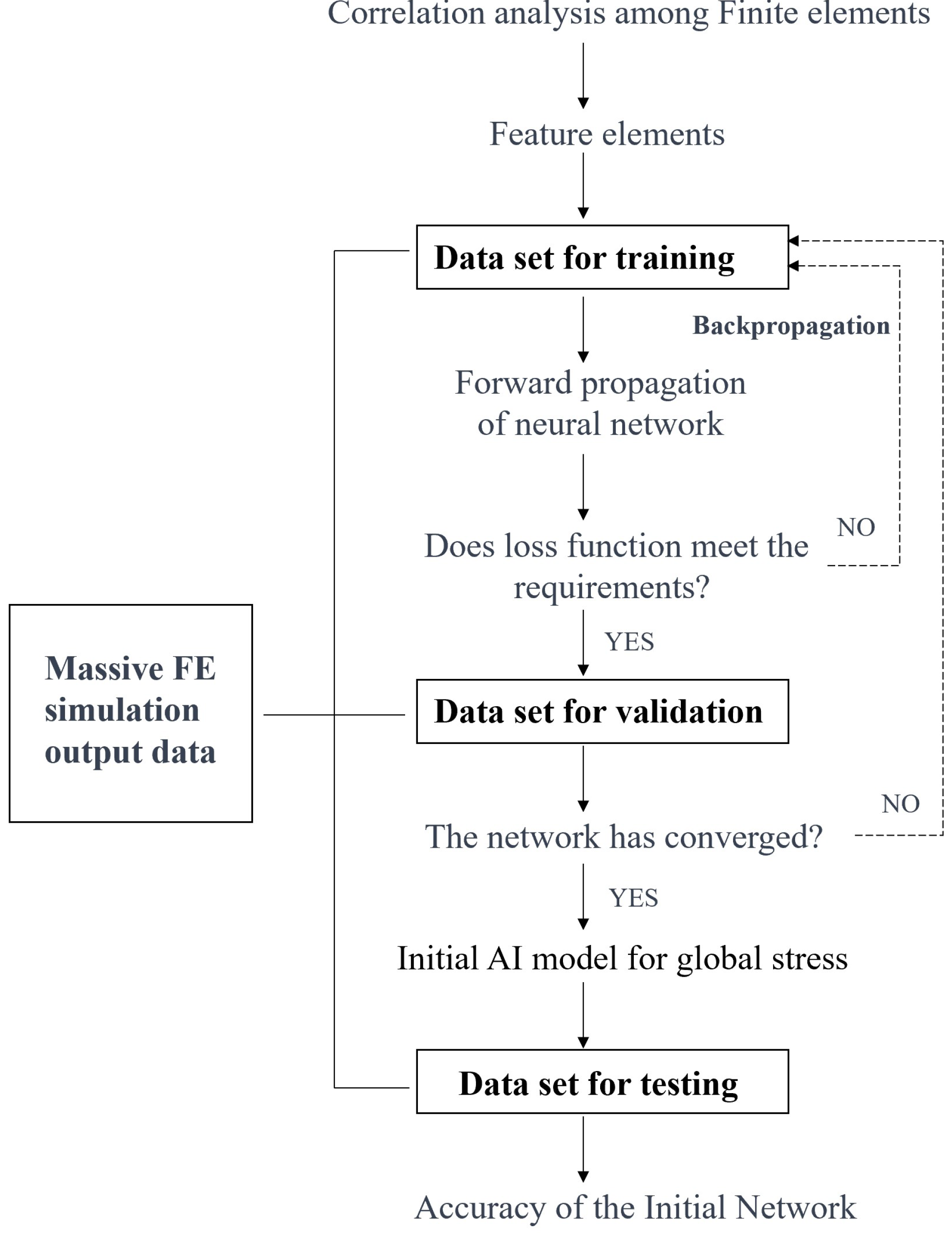
3.2. The Process of Establishing an ANN for Global Stress

The process of establishing an ANN involves several key aspects, including data sample planning, a feedforward neural network architecture, backpropagation, convergence assessment, and a generalization performance evaluation. These aspects will be explored in detail through specific case studies. Figure 1 offers a concise overview of the process involved in constructing an ANN for the reconstruction of global stress. The following workflow is proposed.

(1)

Acquire Sufficient Training Data [22]: Obtain ample training data since direct measurements of spatial structural global stress are impractical. Finite element simulation data are used as the training sample. These data should be divided into three sets: training, validation, and testing sets.

(2)

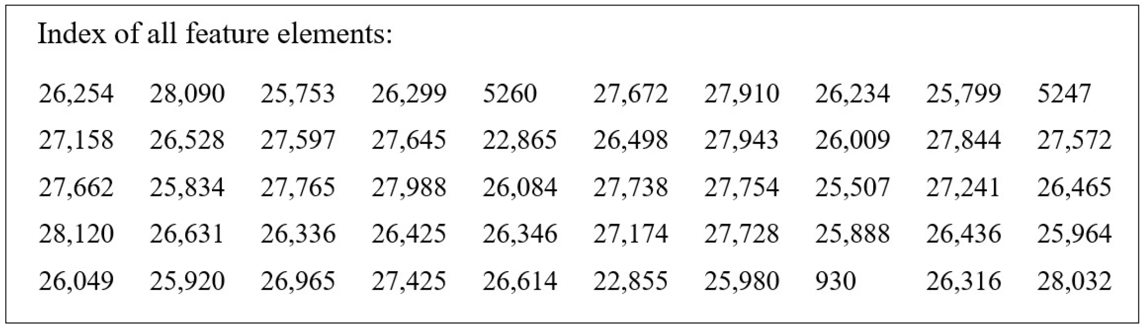
Select Feature Elements: Identify and select the characteristic or representative elements that contribute significantly to the overall stress field. These feature elements will serve as the input to the ANN, and details will be given in Section 4.3.

(3)

Design ANN Architecture [23]: Construct a feedforward neural network architecture specifically tailored to the prediction of global stress. The training set is employed to train the network in capturing global stress. The network is optimized using the backpropagation algorithm with gradient descent, which allows for parameter adjustments to minimize the loss function between predicted and target data.

(4)

Address Convergence and Overfitting [22]: Evaluate the convergence of the ANN during the training process. The validation set assesses the network’s convergence and serves as a basis in determining when to conclude the training process. If the network demonstrates underfitting (insufficient learning) or overfitting (overly adapted to training data), appropriate adjustments and optimizations should be implemented to achieve a balance between accuracy and generalization.

(5)

Evaluate Generalization Performance [24]: Assess the ANN’s ability to generalize by quantifying its prediction accuracy. The test set evaluates the network’s predictive accuracy. Additionally, the dispersion or variability of the network’s predictions of global stress should be quantitatively measured to assess its performance.

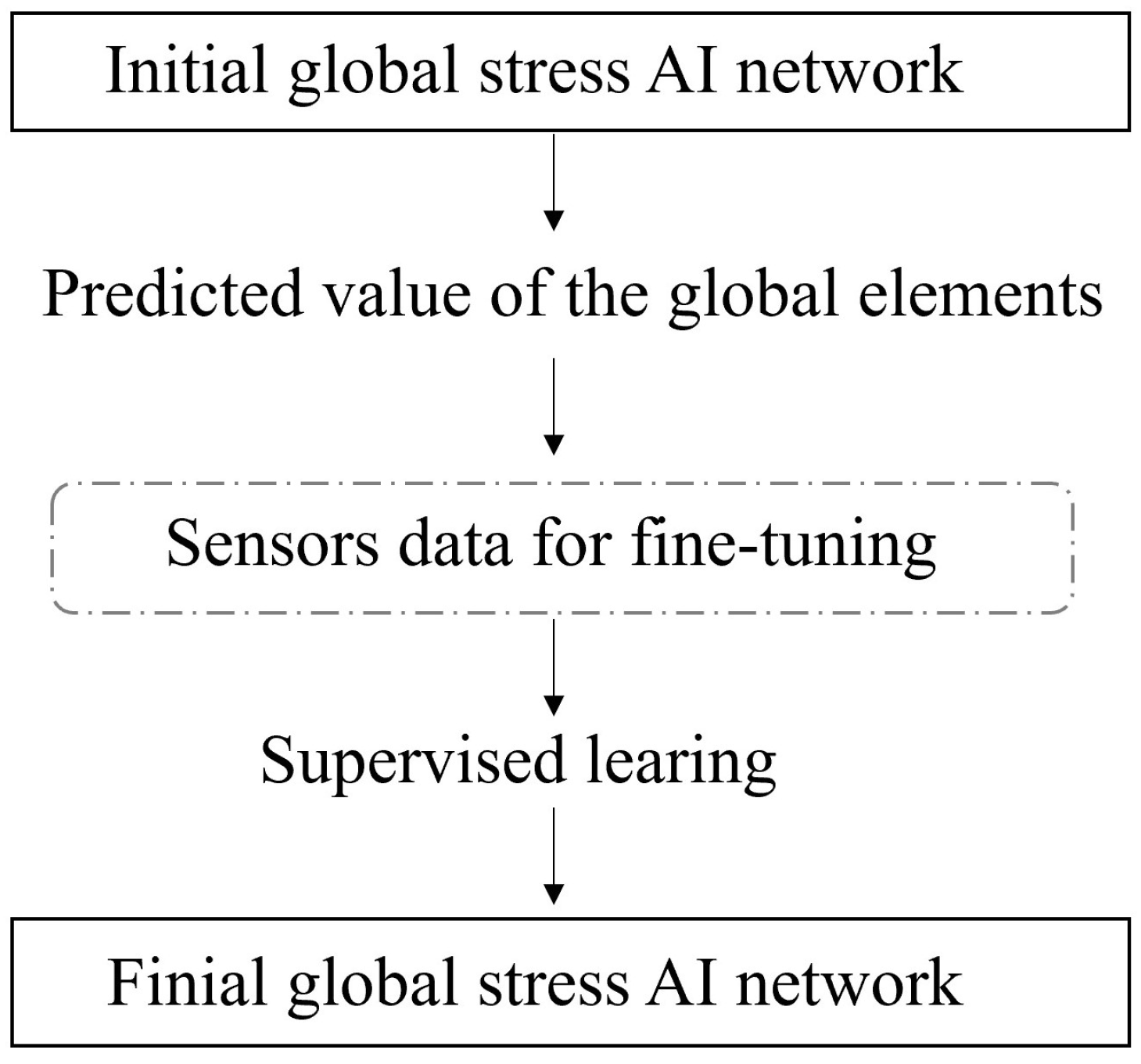
3.3. Fine-Tuning of Initial Network

The ANN for global stress was established using simulation output data, and it requires fine-tuning before it can be deployed to physical structures. The reasons are as follows: (1) there are slight differences between the material properties, boundary conditions, mesh partitioning, load simulation, and other information used in simulation calculations and the real physical world; (2) the actual measurement point location and orientation may have geometric errors compared to the ideal placement state.

Figure 2 illustrates the process of fine-tuning the ANN trained by simulation data (initial network). To fine-tune the initial network for deployment to physical structures, measurement points are randomly selected from areas of high stress. The actual sensor data are compared to the predicted values of the initial network, and a fine-tuning matrix is added outside the output layer of the network through supervised learning. This process creates the final artificial intelligence network (referred to as the “final network”) that can be deployed to physical structures.

The process of fine-tuning the initial network is similar to the process of establishing the initial network, as both require a dataset for error comparison. The goal is to minimize the loss function through optimization algorithms and improve the ANN. The key difference arises in the dataset used for validation, which plays a crucial role in achieving optimal performance.

During the establishment process, the dataset for validation can be easily obtained from simulation output data at a low cost, allowing for a larger number of elements to be used for validation. In this case, any element, apart from the feature and test elements, can be designated for validation purposes. This broad selection of elements facilitates a comprehensive evaluation of the network’s performance.

However, during the fine-tuning process, a much smaller number of elements are available for validation, as they require sensor measurements. This limited number of elements used for validation can potentially lead to the network becoming trapped in local optimization instead of attaining global optimization.

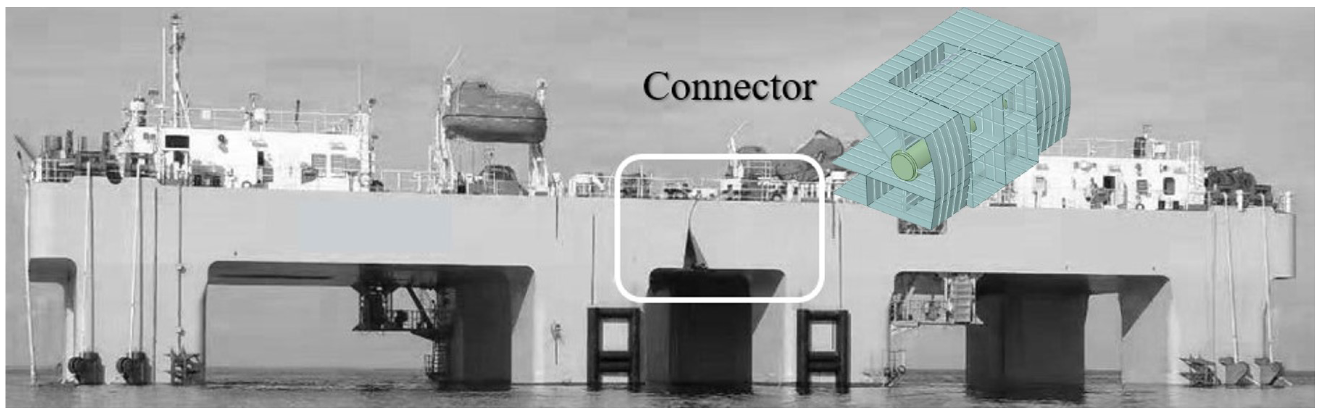
4. Reconstructing Global Stress for a Marine Connector

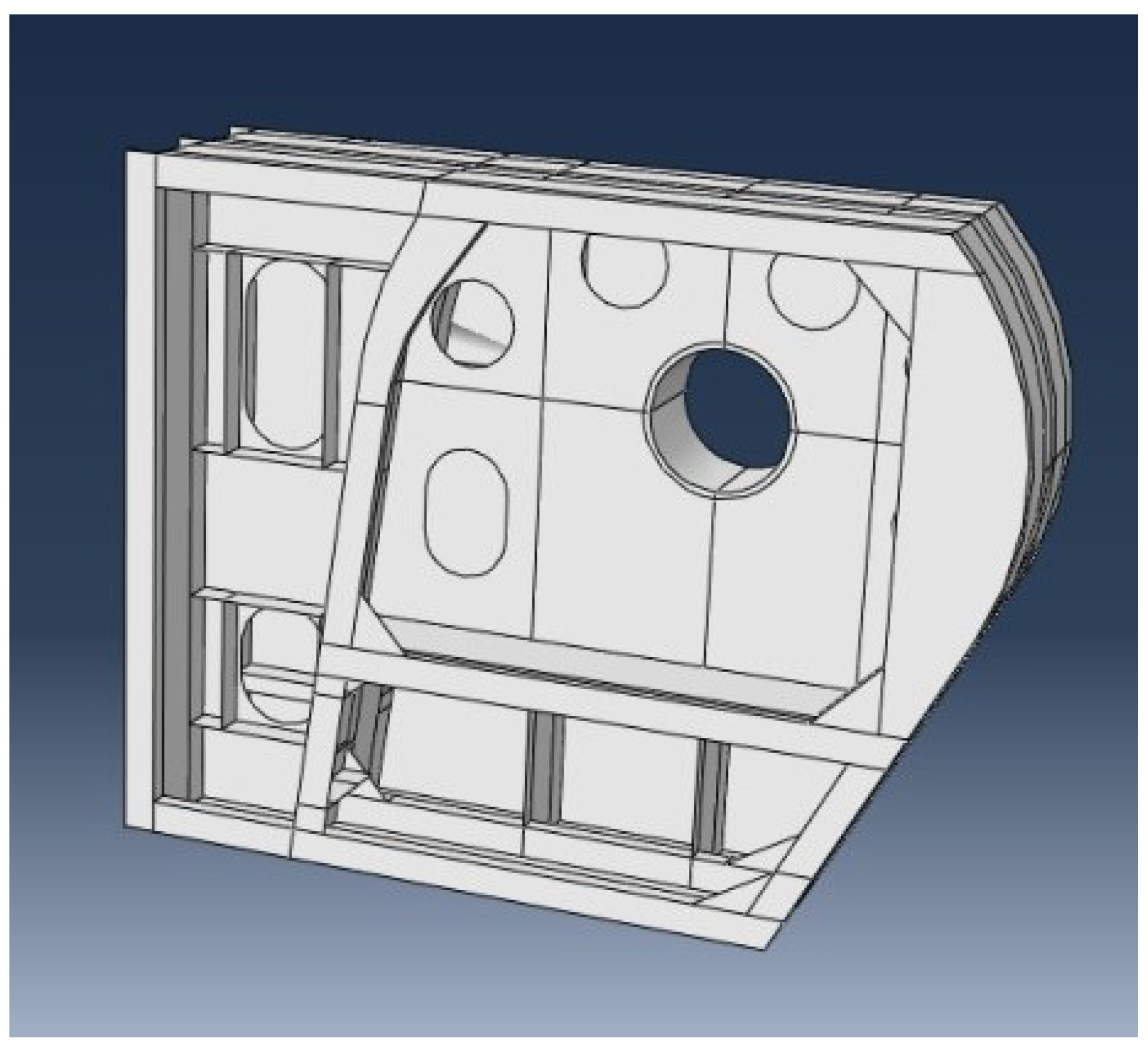
4.1. Description of the Marine Connector Structure

The marine platform consists of two semi-submersible platforms connected by a pin joint, as in Figure 3. Under extreme sea conditions, the pin and connector experience significant shear forces, necessitating a real-time assessment of the structural safety. This study aims to evaluate the safety of the connector structure by employing stress sensors on its surface to obtain a stress distribution map. The map identifies high-stress regions and their magnitudes. The connector structure is categorized into single-ear and double-ear structures, with the focus of this investigation being on the single-ear connector, as in Figure 4. It is a complex three-dimensional curved surface structure composed of three layers of bulkheads, with the middle bulkhead featuring lightening holes.

4.2. Simulation for the Connector

(1)

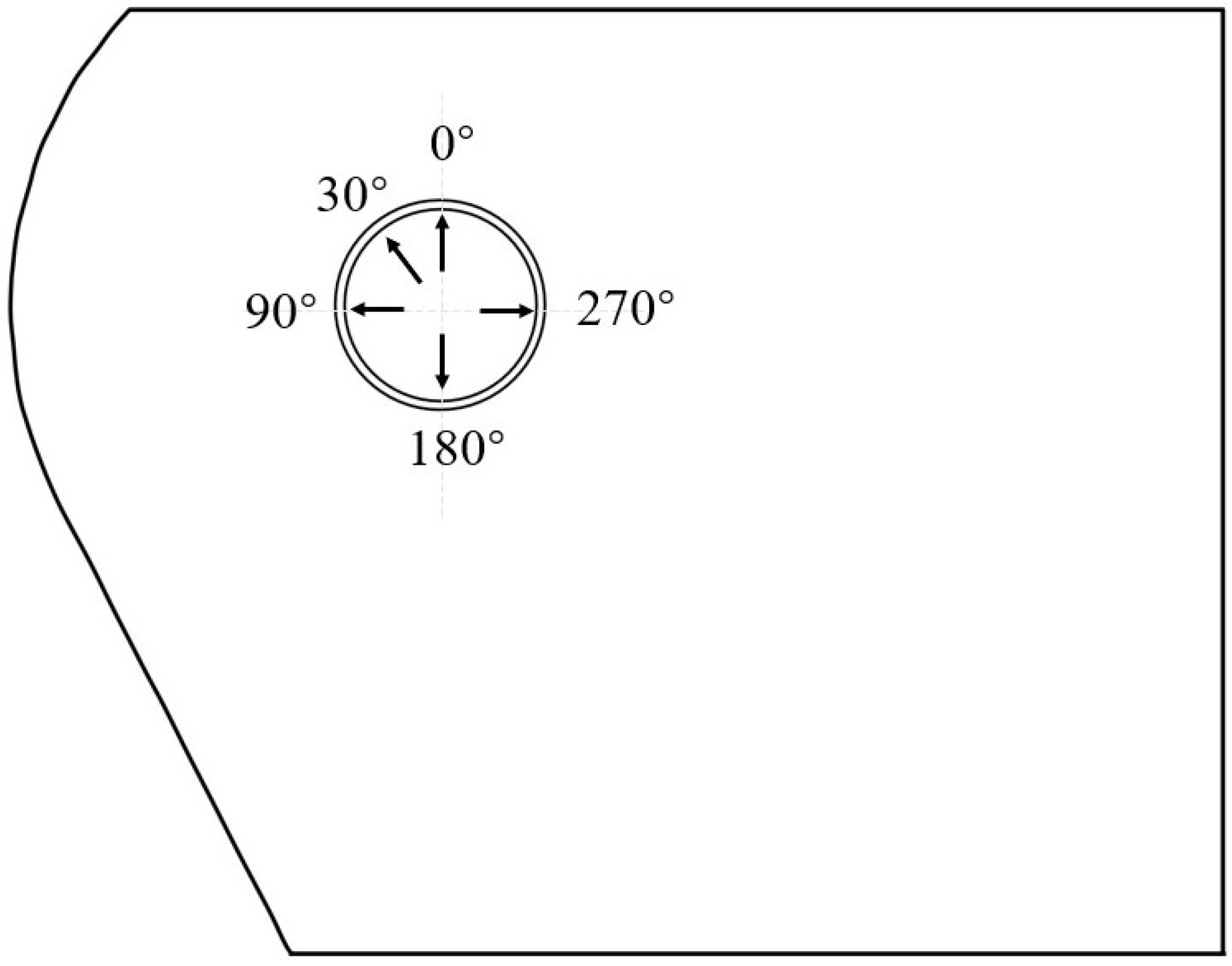
Load Analysis

The THAFTS (version 2.0) software was utilized for the three-dimensional hydroelastic analysis, determining the connector’s response amplitude operator and short-term extreme profile loads [25]. The analysis revealed that the connector experienced primarily longitudinal and vertical forces, with lateral compression as a secondary loading mode. Wave direction greatly influenced the connector load, with oblique waves resulting in the highest loads. The study considered a connector load range of 0 to 2630 kN within the $XY$ plane, representing the primary loading mode [26,27].

(2)

Nonlinear Contact

A finite element model was created in ABAQUS for the simulation analysis of the connector, with different elements used to model the connector body, load-bearing dowel pin, and bearing sleeve.

During the modeling process, a Tie constraint was employed between the bearing seat and the connector, while the contact fit between the dowel pin and the bearing seat was simulated using a penalty function with rigid contact in the normal direction and limited sliding in the tangential direction. The quasi-static nonlinear simulation was conducted using the arc-length method.

In terms of simulation conditions, a block was introduced to simulate the load on the connector, coupled with a reference point (RP3) representing the compression and separation between the main and secondary platforms.

(3)

Calculation Conditions

The load range varied from 50 kN to 5000 kN, with the maximum load approximately twice the design load of 2630 kN. Loads were calculated at 10${}^{\circ }$ intervals, resulting in 3600 load cases across 36 directions. Figure 5 gives a schematic of the load directions.

(4)

Partitioning of Data Samples

Due to the contact connection between connectors and pins, the global stress gradient does not linearly increase and distribute along the load magnitude under different load conditions with varying amplitudes and angles [28].

All the finite element stress data for all load cases are used as sample data, and they are randomly divided into training sets (2400 cases), validation sets (600 cases), and test sets (600 cases). These data from the simulation will be utilized to build the initial ANN for global stress.

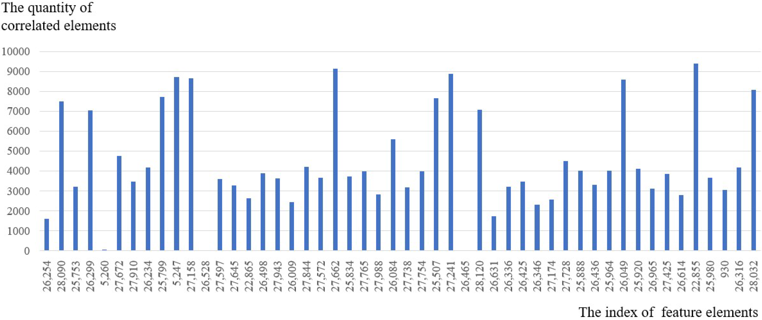
4.3. Selecting Feature Elements by Correlation Analysis

The overall finite elements are subjected to a correlation analysis using the Pearson correlation coefficient, and the steps are illustrated in Figure 6.

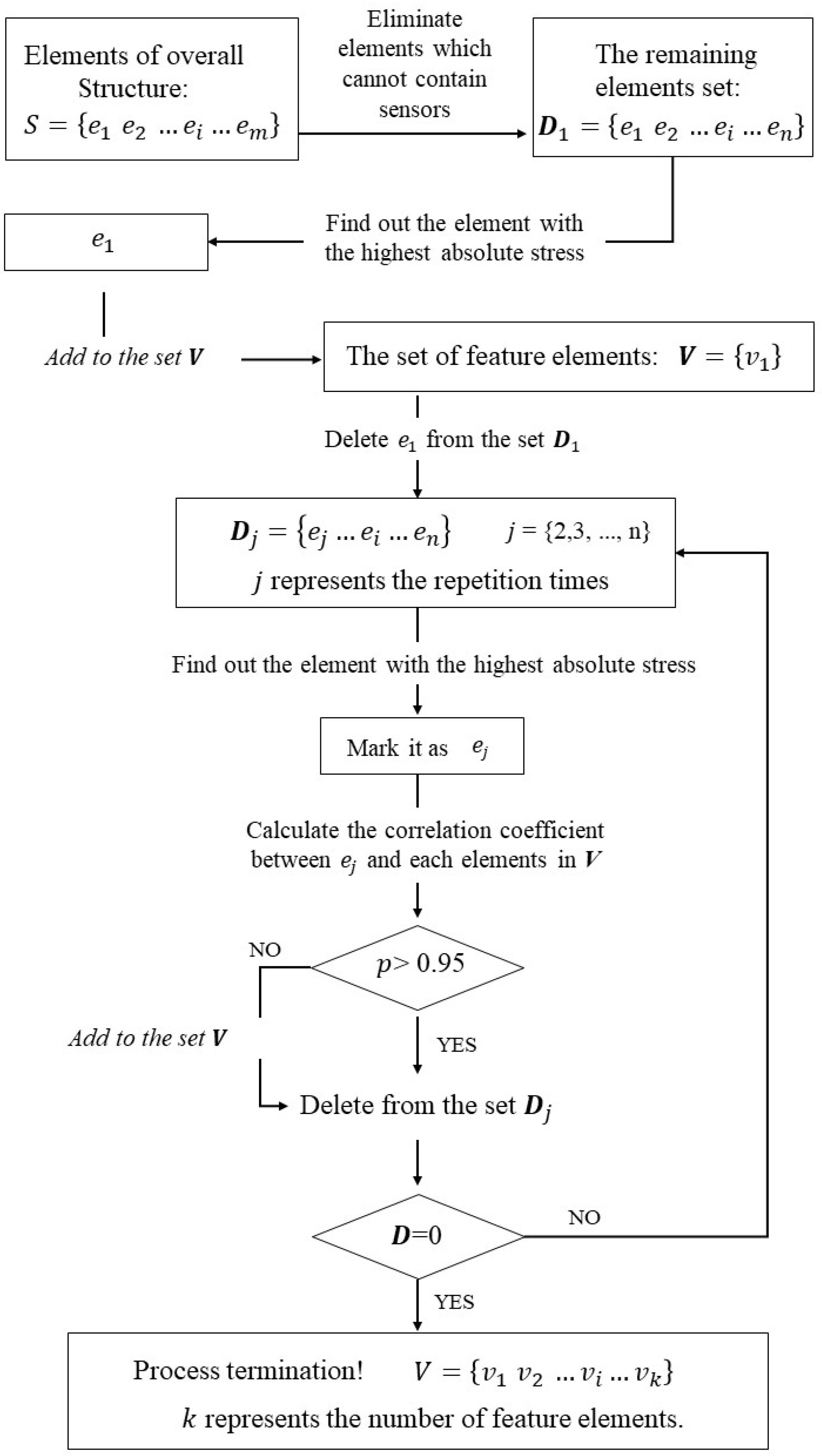
(i)

Eliminate the finite elements that cannot accommodate sensors from the overall structure. Then, sort the remaining finite elements (record the quantity as n in descending order based on their absolute stress values). The greater the absolute stress value, the more sensitive the finite element is to external loads. Placing sensors at these positions is advantageous in detecting minor changes in external loads and structural responses.

(ii)

The finite element with the highest absolute stress value in D is chosen as the feature element $v_1$. Subsequently, the correlation coefficient $p_{ij}$ between $v_i$ and other elements $e_j$ is sequentially calculated, where $j=\{2,...,n\}$, and j represents the repetition times. Based on Equations (4) to (8), the correlation matrix P of the finite element is obtained. If $p_{ij}>0.95$, $e_j$ is added to the set V.

(iii)

The elements in S that are duplicated in V are removed to obtain the remaining set of elements D.

(iv)

Repeat steps (ii) and (iii) until the number of remaining elements in set D reaches 0; then, the selection process is completed.

A total of 50 feature elements have been identified among the 30,858 finite elements. Figure 7 showcases the indexes assigned to these 50 feature elements in the finite element model, with a noteworthy concentration of indices falling within the range of 26,000 to 28,000. This specific region, situated near the contact surface with the pin, corresponds to areas characterized by higher stress gradients. Consequently, this observation provides logical support for the selection of feature elements based on the Pearson correlation coefficient, affirming their alignment with the intricate three-dimensional stress distribution characteristics of the structure.

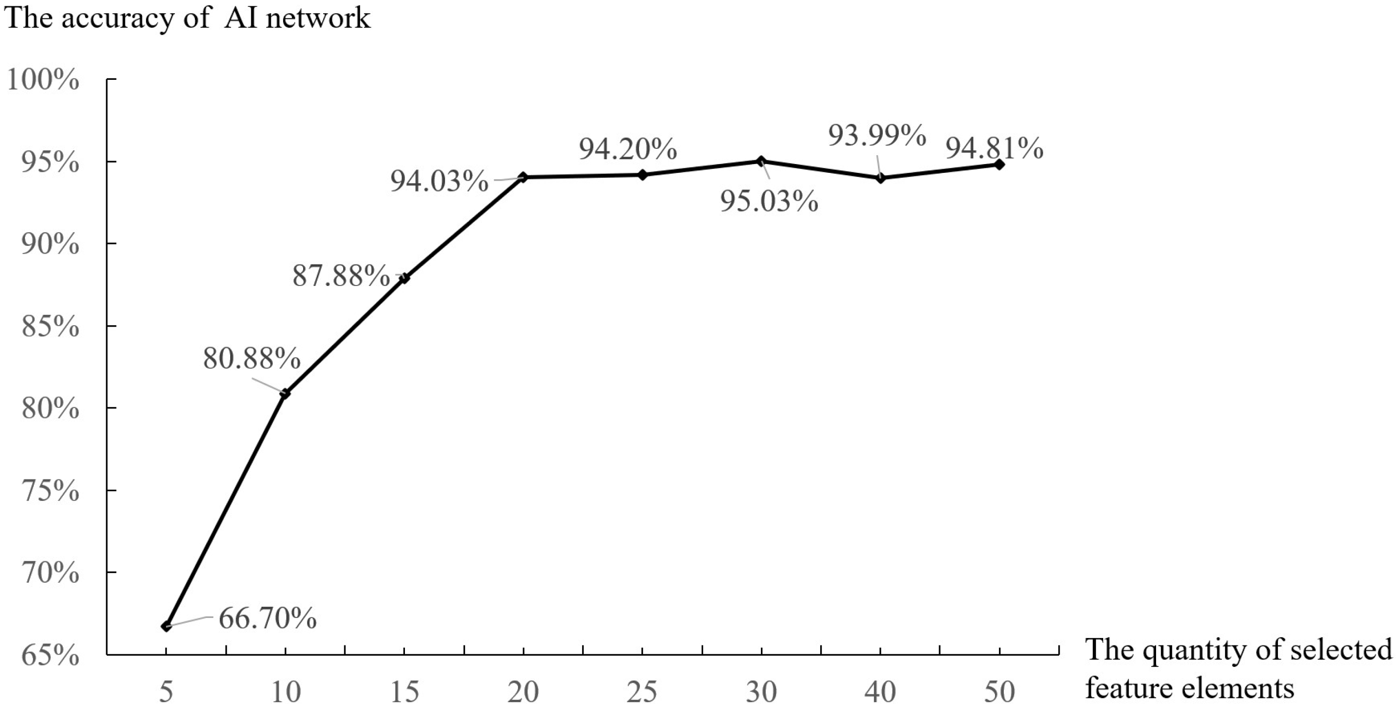
4.4. Optimization of the Number of Stress Sensors

The 50 feature elements were sorted in descending order according to their stress amplitudes, and the number of correlated elements for each feature element was counted, as shown in Figure 8. The results showed that the number of finite elements that had a correlation with the 50 feature elements was 220,905, exceeding the total number of entire elements, which was 30,858. This indicates that there are multiple intersections among the 50 subsets, and fewer feature units can be used to obtain the full-field stress distribution.

Subsequently, a neural network was trained for global stress by selecting 5, 10, 15, 20, 25, 30, 40, and 50 feature elements in descending order of their stress amplitude as input variables. The influence of different numbers of feature elements on the accuracy of the global stress solutions was analyzed, and the results are shown in Figure 9. It was observed that as the number of feature elements gradually increased, the calculation accuracy also improved, and the algorithm’s accuracy was found to be stable when the number of selected feature elements was 20. This indicates that most of the finite elements in the connector structure are strongly correlated with the first 20 feature elements, and the global stress of the connector can be accurately obtained using these 20 feature elements.

4.5. Optimization of Neural Networks

Different neural network architectures exhibit varying computational performance and accuracy in obtaining global stress. To conduct the experiments, four commonly used neural network architectures, namely BP, CNN, RNN, and DNN, were selected. The experiments were based on the same input elements, validation dataset, and convergence conditions. BP was used as the optimized standard network, CNN used the conv2d convolution layer provided by Pytorch, RNN had a sequence size of 3, and DNN used 10 layers of neurons.

Table 1. Comparison of solution accuracy of different neural networks.

	BP	CNN	RNN	DNN
Minimum accuracy	90.4%	85.3%	90.6%	88.9%
Maximum accuracy	94.7%	88.8%	93.4%	94.8%
Number of hidden layers	4	4	1	11

shows the comparison of the algorithmic accuracy of the different networks by the minimum and maximum accuracy achieved using the test dataset.

Table 1 shows that the CNN network has the lowest accuracy, while the BP and RNN networks have slightly lower prediction accuracy than the DNN network. However, the DNN and RNN networks require excessive computational power. On the other hand, the BP network has relatively stable accuracy. Considering both the solution accuracy and computational speed, the BP network outperforms the others.

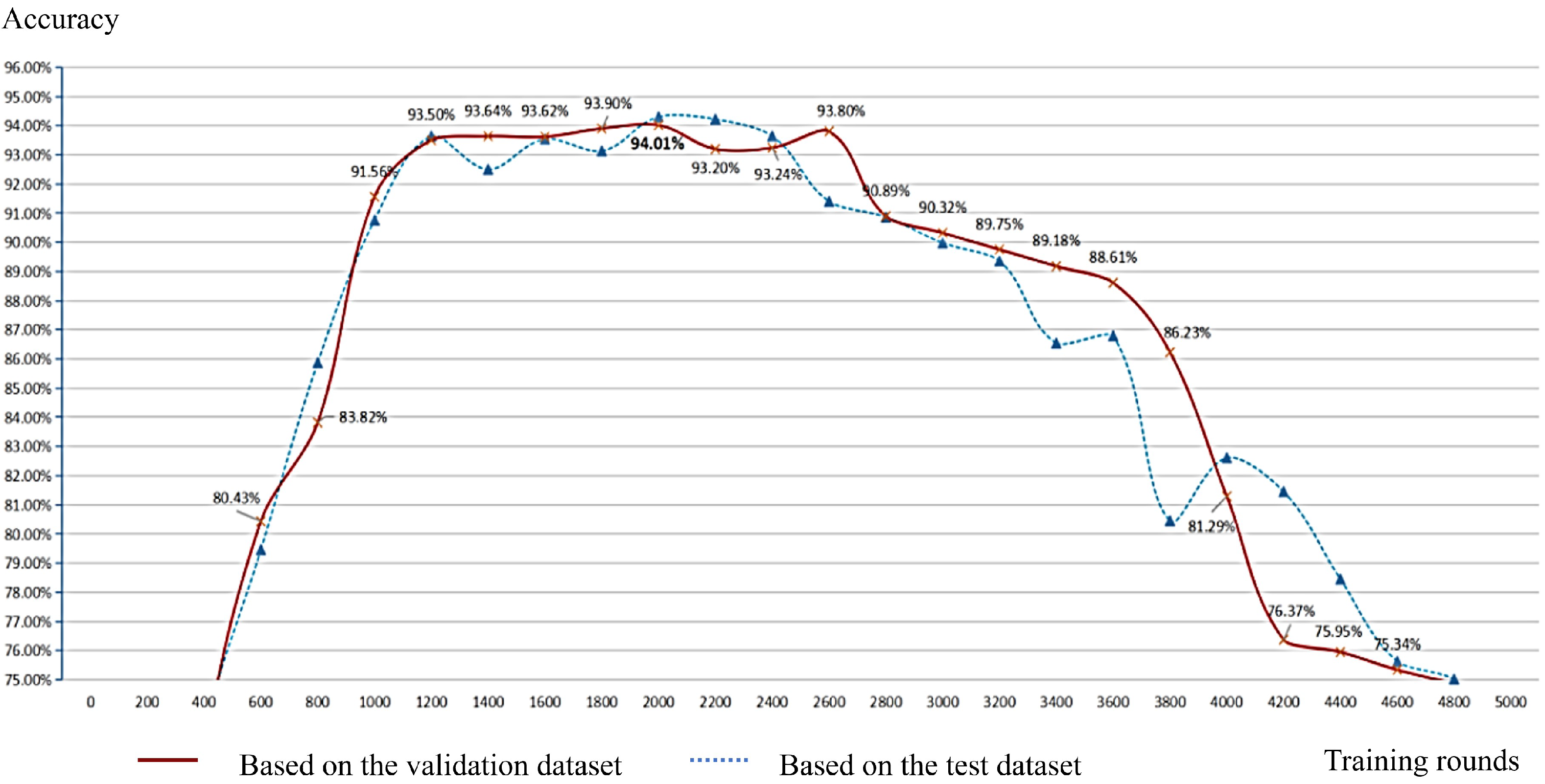
4.6. Convergence of Neural Network

When predicting a large number of output variables with only a small number of input variables, overfitting can occur during the training process of neural networks. Overfitting can cause a decrease in the prediction accuracy of the neural network. Figure 10 shows the curve obtained when training a global stress neural network using the BP neural network without setting a convergence judgment. The horizontal axis represents the training rounds, and the vertical axis represents the accuracy. The blue curve represents the accuracy verified by the validation set every 200 rounds of training, while the red curve represents the accuracy evaluated by the test set every 200 rounds of training.

We can observe the following. (1) As the number of training rounds increases, the prediction accuracy of the network first rises and then becomes flat, and it finally drops sharply, indicating the phenomenon of overfitting. Therefore, it is necessary to design a convergence rule. (2) The consistent performance trends of the validation set and the test set in terms of accuracy demonstrate that the validation set can effectively provide an approximate evaluation of the network’s performance. Therefore, the following convergence rules should be set when training the neural network to obtain the global stress of the connector structure: when the accuracy of the network verified by the validation set decreases by more than 5%, the network should stop training and the previously trained network should be used as the final network established by the simulation data. 2000 has been chosen as the round times to stop training, achieving a predictive accuracy of 94.01%.

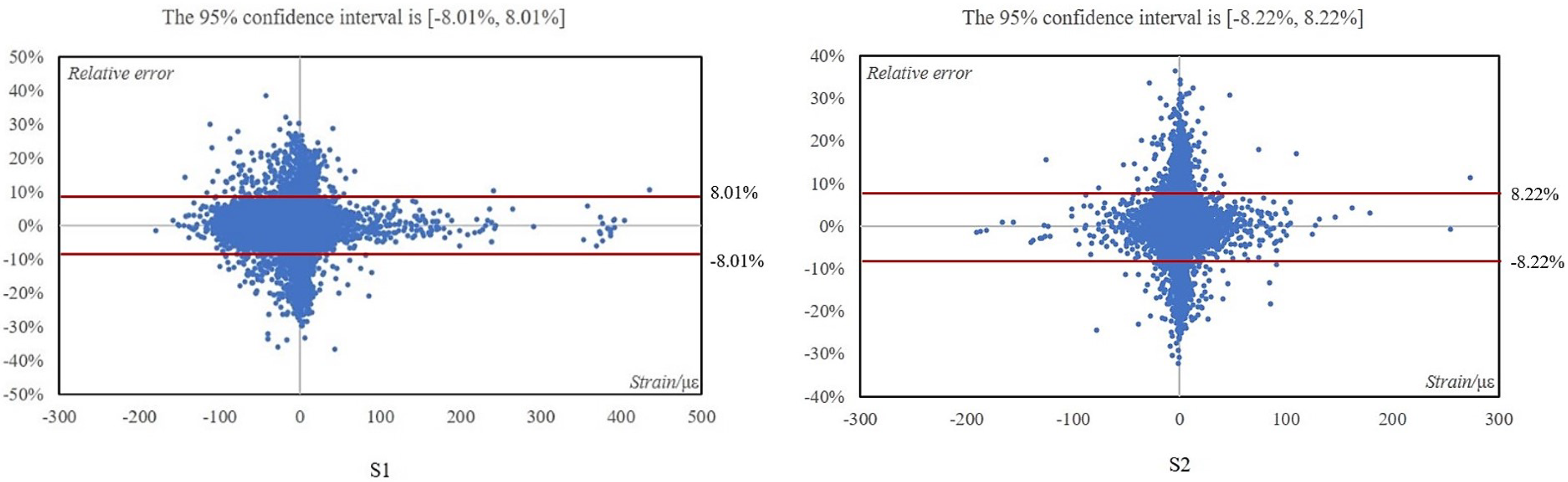
4.7. Uncertainty Analysis of the ANN Based on Simulation Data

An uncertainty analysis was conducted on the initial ANN for the global stress of connectors based on 600 test datasets. Figure 11 displays the relative error distribution of the remaining 30,838 elements’ stress values that were obtained using 20 feature elements’ stress values as inputs, under the working condition of 420 tons of shear force and a direction of 60${}^{\circ }$. (The shear force is considered zero when it is vertical, and a counter-clockwise direction is considered positive.) The abscissa denotes the magnitude of stress, and the ordinate represents the relative error. The results show that in the S1 direction, 95% of the finite elements’ stress values were predicted with an error range of [−8.01%, 8.01%]. Similarly, in the S2 direction, 95% of the finite element stress values were predicted with an error range of [−8.22%, 8.22%] [29].

5. Verifying Accuracy via Physical Structure Test

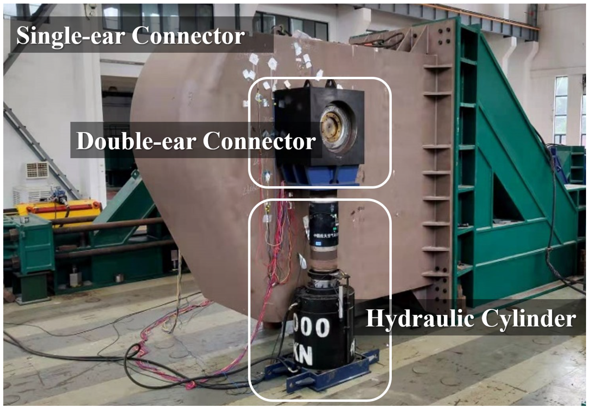
5.1. Physical Test Object

The stress values in the sensor-free areas are generated by AIGC. To verify the accuracy of the ANN in obtaining the global stress of the connector structure, physical structural tests were conducted using a 1:1 model. The main parameters of the single-ear connector model are presented in

Table 2. Main parameters of the connector model.

Principal dimension	Length	3.95 m
Principal dimension	Width	1.70 m
Principal dimension	Height	3.20 m
Material	Double-ear connector (the fixture)	42CrMo steel (yield strength 450 MPa)
Material	Single-ear connector	ZG230-450H steel (yield strength 240 MPa)

.

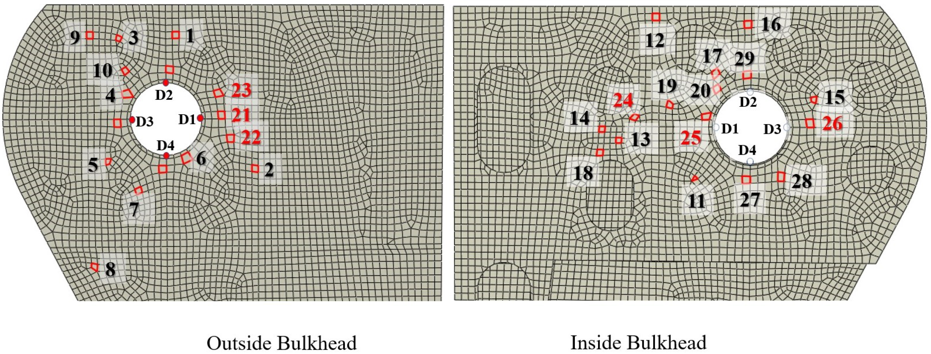
5.2. Arrangement of the Stress Sensors

Static strain gauges and a total of 29 three-dimensional stress sensors were utilized for the test, as depicted in Figure 12. The sensors numbered 1 to 20 were utilized for training and were strategically positioned at feature elements to provide input data for the ANN. Sensors numbered 21 to 26 were strategically placed in high-stress areas of the outer and intermediate bulkheads to fine-tune the ANN. Lastly, sensors numbered 27 to 29 were used for verification purposes and were placed in arbitrary positions within the high-stress area.

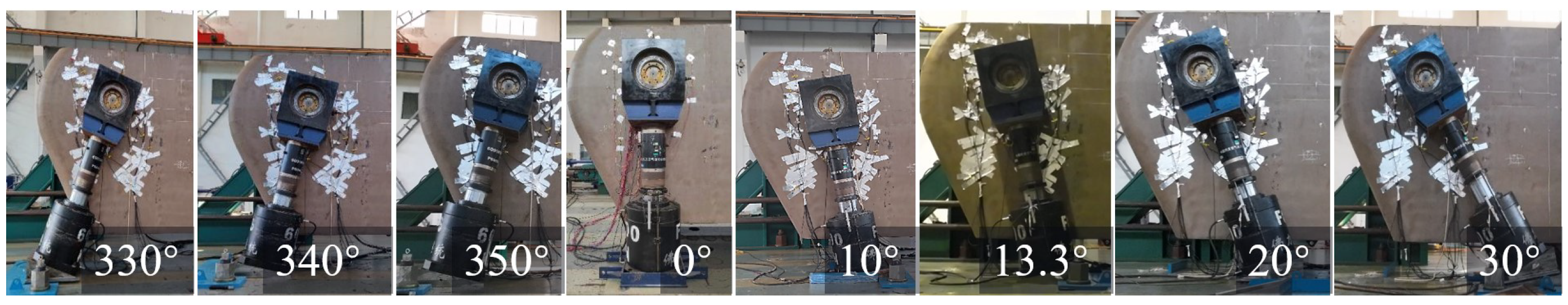
5.3. Process of the Test

A fixture was utilized to simulate the adjacent double-ear connector, while a hydraulic cylinder was used to apply simulated shear forces. Precise control of the shear force was achieved using a force sensor, with the inclined angle simulated by fixing a bottom block to the cylinder, as shown in Figure 13 and Figure 14. The test was conducted within the elastic ranges, and the loading scheme is presented in

Table 3. Detailed loading conditions.

	Fine-Tuning Loading Scheme (kN)			Validation Loading Scheme (kN)
Angle	Min Load	Max Load	Load Step	Min Load	Max Load	Load Step
0${}^{\circ }$	1000	2000	100	2000	2500	50
10${}^{\circ }$	100	1300	100	100	1300	50
13.3${}^{\circ }$	\	\	\	100	1300	50
20${}^{\circ }$	100	1300	100	100	1300	50
30${}^{\circ }$	100	1300	100	100	1300	50
330${}^{\circ }$	100	1300	100	100	1300	50
340${}^{\circ }$	100	1300	100	100	1300	50
350${}^{\circ }$	100	1300	100	100	1300	50

. During the fine-tuning phase, the load conditions were distinct from those used for accuracy verification. A total of eight loading experiments were conducted at various angles. Among them, an angle of 13.3${}^{\circ }$ was randomly selected as a test condition, and the corresponding measured data were excluded from the training process. Instead, they were specifically employed to evaluate the accuracy of the ANN in predicting global stress.

5.4. Test Results

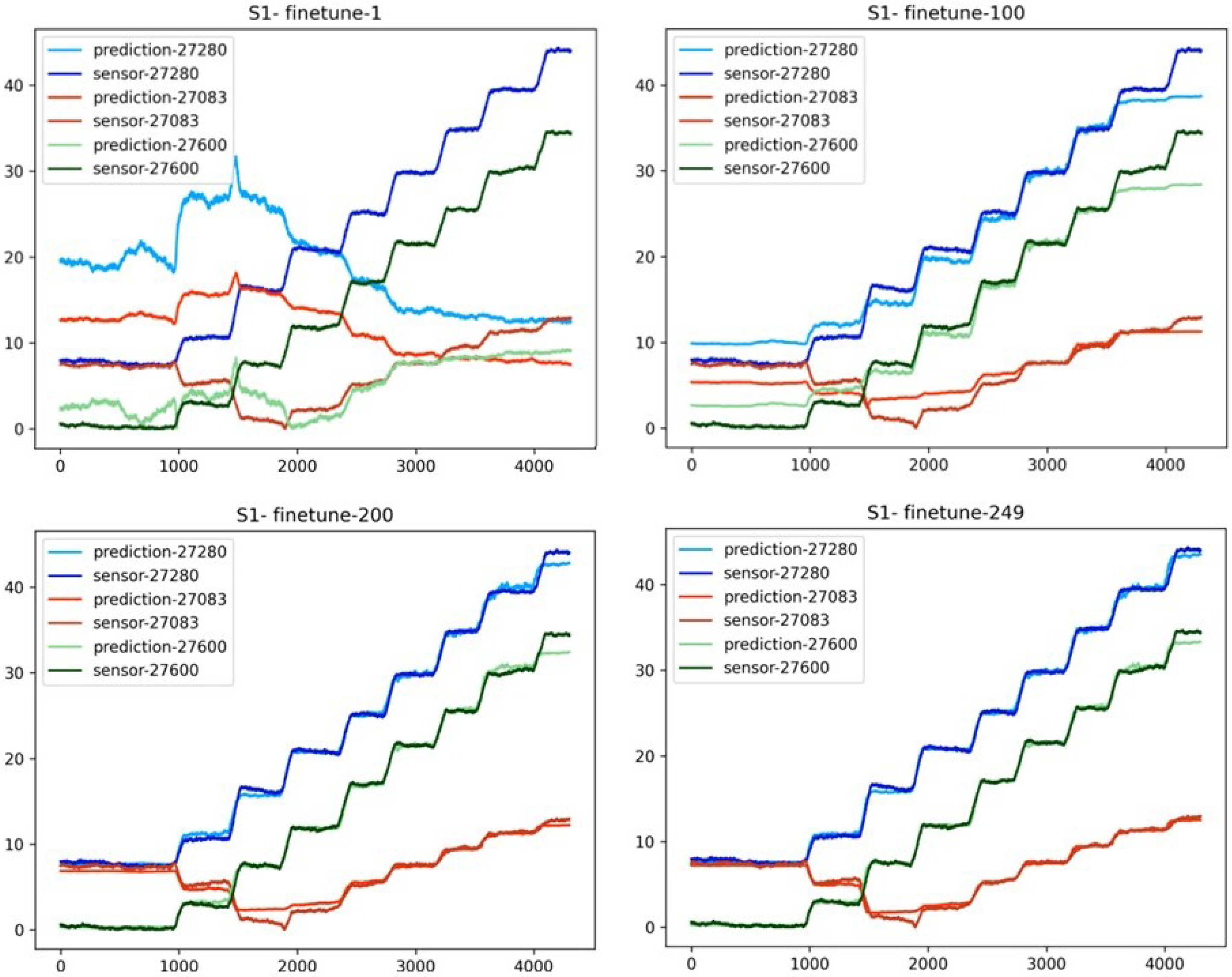
(i)

Figure 15 illustrates the process of fine-tuning a neural network at a loading angle of 10${}^{\circ }$. The horizontal axis represents the experimental time steps, and the vertical axis represents the measured stress values. The neural network generates the stress data for three randomly selected validation elements; after 249 rounds of fine-tuning, the neural network can accurately predict the stress value.

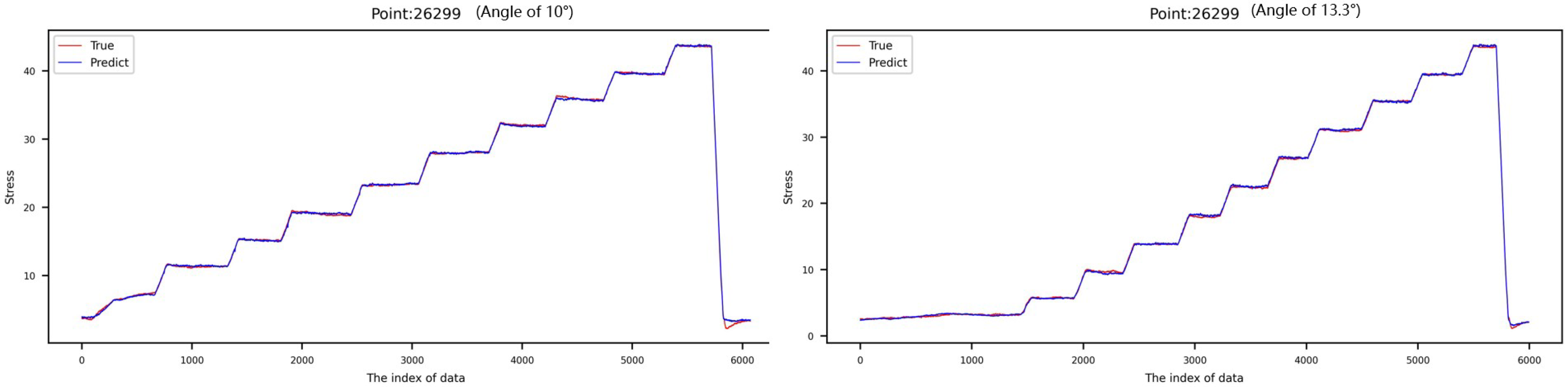
(ii)

Experimental data within the load range of 800 to 1200 kN were collected at two different shearing force angles: 10${}^{\circ }$ and 13.3${}^{\circ }$. For the 10${}^{\circ }$ angle, some of the data underwent fine-tuning with an ANN previously. The stress values generated by the ANN at the validation element (Index No. 26299) were compared to the actual measured values. In contrast, for the 13.3${}^{\circ }$ angle, the data were not trained or fine-tuned with the ANN. The stress values predicted by the ANN at the validation point were again compared to the actual measured values (see Figure 16). Both comparisons provide insights into the accuracy and effectiveness of the ANN in predicting stress values under different shear force angles.

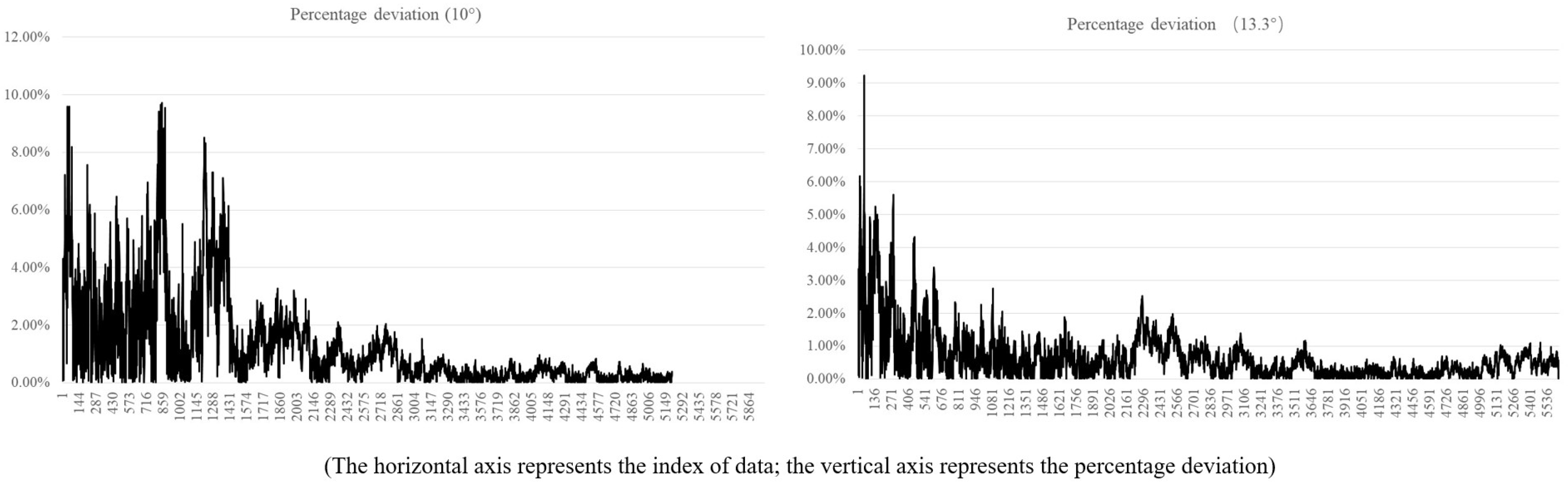
(iii)

The percentage deviation between the ANN-generated values and the actual measured values for the validation element (Index No. 26299) was plotted as a fluctuation graph along the index of data (see Figure 17). Notably, the percentage deviation remained consistently below 10% for both conditions, with an overall average below 4%. This indicates the robustness of the ANN in accurately predicting the connector’s global stress, affirming its reliability under different load conditions.

A real-time global stress viewer for the connector was developed and integrated into the SHM system using the fine-tuned neural network. Figure 18 illustrates the global stress obtained by the system under a vertical shear force of 1936 kN. Regarding the physical properties, it is impossible to achieve an exact match between the values generated by AIGC and the actual measurement for all elements. Therefore, the focus should be on the accuracy of the ANN in identifying high-stress positions and magnitudes.

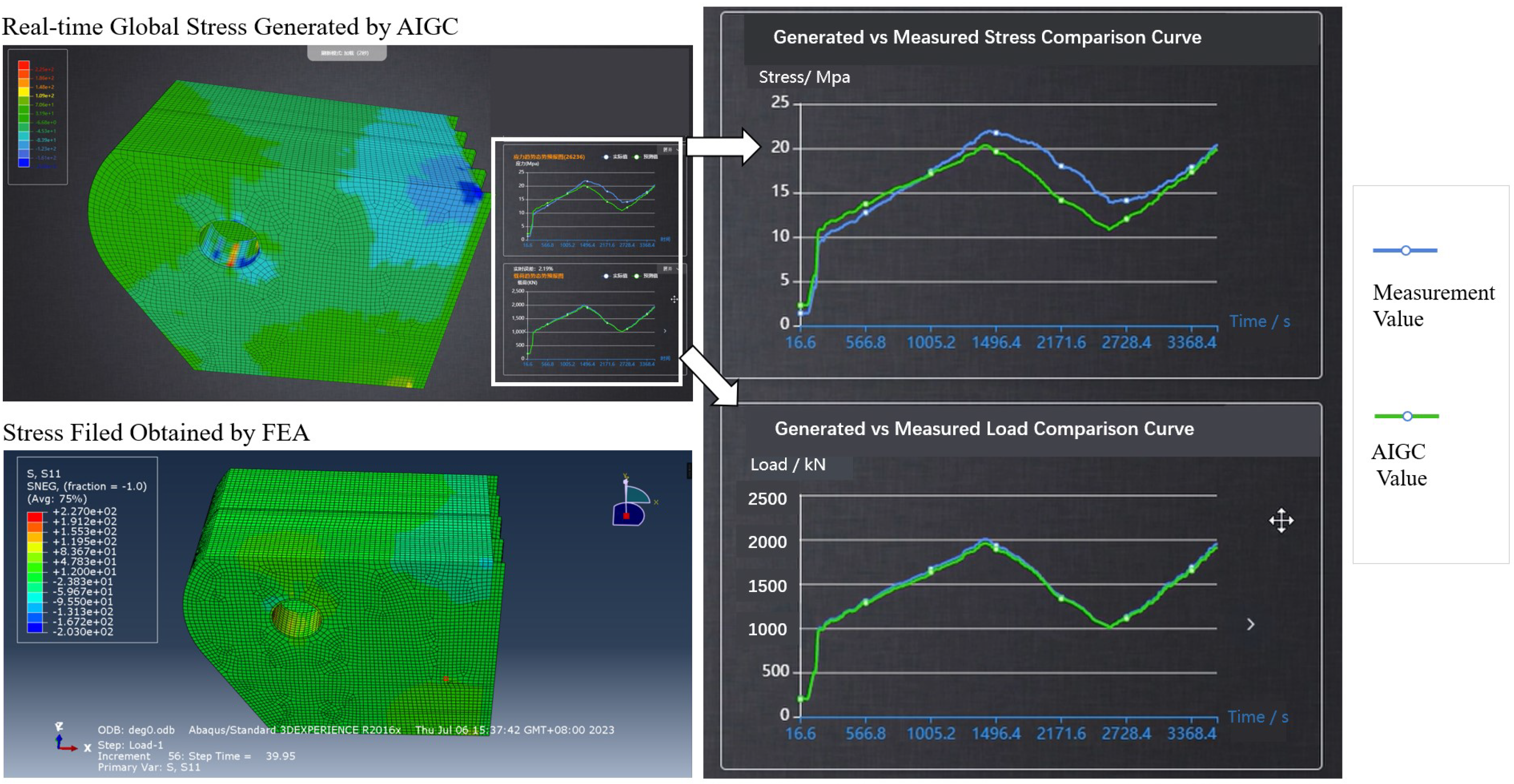
(i)

The software effectively identifies the load direction as vertically upward, with the maximum stress located beneath the pinhole of the connector. Additionally, high-stress areas are recognized on both sides and the upper portion of the pinhole. Moreover, as one moves away from the pinhole, the stress amplitude of the structure decreases, which is consistent with the contour map obtained through Finite Element Analysis (FEA). This consistency demonstrates adherence to the principles of mechanics.

(ii)

The comparison curve between the measured stress values and the stress values generated by AIGC indicates overall solution accuracy as high as 93.6%.

6. Conclusions

This paper proposes an innovative approach to obtaining the real-time global stress of marine structures with a limited number of stress sensors using AIGC. By dividing the spatial structure into correlated subsets of finite elements, feature elements are selected as stress measurement points. Individually, these feature elements exhibit low correlation, but, when combined, they effectively capture the overall state of the structure. Subsequently, an ANN is employed to establish the relationship between the feature elements and their corresponding subsets, enabling the reconstruction of the global stress of the structure.

A neural network is established based on FE simulation data using 20 feature elements as input variables to predict the remaining 30,858 element data. Uncertainty analysis demonstrates that 95% of the elements have solution errors within 9% [29]. The accuracy of the proposed method is validated through the physical structural model test. The fine-tuned ANN consistently generates stress for both 10${}^{\circ }$ and 13.3${}^{\circ }$ shear force angles, with deviations below 10% and an average deviation of less than 4%.

These results highlight the feasibility and strong generalization performance of the method in enhancing traditional SHM systems. While this study provides insights into real-time stress field solutions in marine structures, further research is needed. Future directions include investigating the impact of different correlation coefficients on the description of complex structures and optimizing the neural network for improved performance. Additionally, it is crucial to identify a suitable evaluation method to ensure the reliability of the data generated by AIGC in engineering applications.

References

- Zhang, T.; Wei, P.; Yue, Y. Resistance Spot Welding Method for Metal-Based Fiber Bragg Grating Sensors. Trans. Nanjing Univ. Aeronaut. Astronaut. 2015, 3, 289–296. [Google Scholar]
- Foss, G.C.; Haugse, E.D. Using Modal Test Results to Develop Strain to Displacement Transformations. In Proceedings of the 13th International Modal Analysis Conference, Society of Photo-Optical Instrumentation Engineers (SPIE) Conference Series, Nashville, TN, USA, 13–16 February 1995; Volume 2460, p. 112. [Google Scholar]
- Ko, W.L.; Richards, W.L.; Tran, V.T. Displacement Theories for In-Flight Deformed Shape Predictions of Aerospace Structures; Technical Report; NASA: Washington, DC, USA, 2007. [Google Scholar]
- Ko, W.L.; Richards, W.L.; Fleischer, V.T. Applications of Ko Displacement Theory to the Deformed Shape Predictions of the Doubly-Tapered Ikhana Wing; Technical Report; NASA: Washington, DC, USA, 2009. [Google Scholar]
- Ko, W.L.; Fleischer, V.T. Extension of Ko Straight-Beam Displacement Theory to Deformed Shape Predictions of Slender Curved Structures; Technical Report; NASA: Washington, DC, USA, 2011. [Google Scholar]
- Tessler, A. A Variational Principle for Reconstruction of Elastic Deformations in Shear Deformable Plates and Shells; National Aeronautics and Space Administration, Langley Research Center: Hampton, VA, USA, 2003. [Google Scholar]
- Tessler, A.; Spangler, J.L. Inverse FEM for full-field reconstruction of elastic deformations in shear deformable plates and shells. In Proceedings of the 2nd European Workshop on Structural Health Monitoring, Munich, Germany, 7–9 July 2004. [Google Scholar]
- Tessler, A.; Spangler, J.L. A least-squares variational method for full-field reconstruction of elastic deformations in shear-deformable plates and shells. Comput. Methods Appl. Mech. Eng. 2005, 194, 327–339. [Google Scholar] [CrossRef]
- Tessler, A. Structural analysis methods for structural health management of future aerospace vehicles. In Key Engineering Materials; Trans Tech Publications: Zurich, Switzerland, 2007; Volume 347, pp. 57–66. [Google Scholar]
- Kefal, A.; Mayang, J.B.; Oterkus, E.; Yildiz, M. Three dimensional shape and stress monitoring of bulk carriers based on iFEM methodology. Ocean Eng. 2018, 147, 256–267. [Google Scholar] [CrossRef]
- Kefal, A.; Oterkus, E.; Tessler, A.; Spangler, J.L. A quadrilateral inverse-shell element with drilling degrees of freedom for shape sensing and structural health monitoring. Eng. Sci. Technol. Int. J. 2016, 19, 1299–1313. [Google Scholar] [CrossRef]
- Ke, Z.; Shenfang, Y.; Yuanqiang, R. Shape reconstruction of self-adaptive morphing wings’ fish bone based on inverse finite element method. Acta Aeronaut. Astronaut. Sin. 2020, 41, 250–260. [Google Scholar]
- Oh, B.K.; Park, H.S.; Glisic, B. Prediction of long-term strain in concrete structure using convolutional neural networks, air temperature and time stamp of measurements. Autom. Constr. 2021, 126, 103665. [Google Scholar] [CrossRef]
- Ye, X.; Chen, X.; Lei, Y.; Fan, J.; Mei, L. An integrated machine learning algorithm for separating the long-term deflection data of prestressed concrete bridges. Sensors 2018, 18, 4070. [Google Scholar] [CrossRef] [PubMed]
- Dai, H.; Zhang, H.; Wang, W. A multiwavelet neural network-based response surface method for structural reliability analysis. Comput.-Aided Civ. Infrastruct. Eng. 2015, 30, 151–162. [Google Scholar] [CrossRef]
- Liu, J.H.; Cheng, J.S.; Chen, J.P. Support vector machine training algorithm: A review. Inform. Control-Shenyang 2001, 31, 45–50. [Google Scholar]
- Zhang, T.; Hu, J.; Wang, X.; Chen, G.; Zhu, Q.; Jiang, Z.; Wang, Z. Solving approach for global stress field of the 3D Structures based on artificial intelligence. Ship Mech. 2023, 27, 238–249. [Google Scholar]
- Lu, W.; Peng, Q.; Cui, Y.; Huang, Z.; Teng, J.; Hu, W. Structural response estimation method based on particle swarm optimisation/support vector machine and response correlation characteristics. Measurement 2020, 160, 107810. [Google Scholar] [CrossRef]
- Zhang, H.; Ji, B.; Liu, S. Digital twin mechanism model for the structural safety of pipelines in geohazards area. Oil Gas Storage Transp. 2021, 10, 1099–1104. [Google Scholar]
- Cooper, S.B.; DiMaio, D. Static load estimation using artificial neural network: Application on a wing rib. Adv. Eng. Softw. 2018, 125, 113–125. [Google Scholar] [CrossRef]
- Schober, P.; Boer, C.; Schwarte, L.A. Correlation coefficients: Appropriate use and interpretation. Anesth. Analg. 2018, 126, 1763–1768. [Google Scholar] [CrossRef] [PubMed]
- Huang, Z.; Shimeld, J.; Williamson, M.; Katsube, J. Permeability prediction with artificial neural network modeling in the Venture gas field, offshore eastern Canada. Geophysics 1996, 61, 422–436. [Google Scholar] [CrossRef]
- Kassa, Y.; Zhang, J.; Zheng, D.; Wei, D. A GA-BP hybrid algorithm based ANN model for wind power prediction. In Proceedings of the 2016 IEEE Smart Energy Grid Engineering (SEGE), IEEE, Oshawa, ON, Canada, 21–24 August 2016; pp. 158–163. [Google Scholar]
- Behzad, M.; Asghari, K.; Eazi, M.; Palhang, M. Generalization performance of support vector machines and neural networks in runoff modeling. Expert Syst. Appl. 2009, 36, 7624–7629. [Google Scholar] [CrossRef]
- Shi, Q.; Zhang, H.; Xu, D.; Qi, E.; Tian, C.; Ding, J.; Wu, Y.; Lu, Y.; Li, Z. Experimental validation of network modeling method on a three-modular floating platform model. Coast. Eng. 2018, 137, 92–102. [Google Scholar] [CrossRef]
- Miao, Y.; Cheng, X.; Ding, J.; Tian, C.; Zhang, Z. Investigation on hydrodynamic performance of a two-module semi-submersible offshore platform. Ships Offshore Struct. 2022, 17, 607–618. [Google Scholar] [CrossRef]
- Zhang, H.; Xu, D.; Lu, C.; Qi, E.; Tian, C.; Wu, Y. Connection effect on amplitude death stability of multi-module floating airport. Ocean Eng. 2017, 129, 46–56. [Google Scholar] [CrossRef]
- Tang, M.; Zhang, Z.; Guo, Z.; Ding, J.; Qi, E.; Gu, X. Design and Assessment Approach of Flexible Connectors for a Double-module Semisubmersible Platform near Island and Reef. In Proceedings of the 29th International Ocean and Polar Engineering Conference, OnePetro, Honolulu, HI, USA, 25–30 June 2019. [Google Scholar]
- Zhu, Q.; Zhang, T.; Wang, X.; Jiang, Z.; Yue, Y. A model of structural stress reverse deduction and its uncertainty quantitative analysis. Equip. Environ. Eng. 2023, 20, 69–76. [Google Scholar]