Abstract
Coal is expected to be an important energy resource for some developing countries in the coming decades; thus, the rapid classification and qualification of coal quality has an important impact on the improvement in industrial production and the reduction in pollution emissions. The traditional methods for the proximate analysis of coal are time consuming and labor intensive, whose results will lag in the combustion condition of coal-fired boilers. However, laser-induced breakdown spectroscopy (LIBS) assisted with machine learning can meet the requirements of rapid detection and multi-element analysis of coal quality. In this work, 100 coal samples from 11 origins were divided into training, test, and prediction sets, and some clustering models, classification models, and regression models were established for the performance analysis in different application scenarios. Among them, clustering models can cluster coal samples into several clusterings only by coal spectra; classification models can classify coal with labels into different categories; and the regression model can give quantitative prediction results for proximate analysis indicators. Cross-validation was used to evaluate the model performance, which helped to select the optimal parameters for each model. The results showed that K-means clustering could effectively divide coal samples into four clusters that were similar within the class but different between classes; naive Bayesian classification can distinguish coal samples into different origins according to the probability distribution function, and its prediction accuracy could reach 0.967; and partial least squares regression can reduce the influence of multivariate collinearity on prediction, whose root mean square error of prediction for ash, volatile matter, and fixed carbon are 1.012%, 0.878%, and 1.409%, respectively. In this work, the built model provided a reference for the selection of machine learning methods for LIBS when applied to classification and qualification.
1. Introduction
Coal is a popular fuel due to its high heat value and low price in some developing countries, although it has some pollution emissions. The quality of the coal has a significant influence on boiler efficiency and pollution emissions; thus, it is necessary to fully grasp the proximate analysis of coal for coal-fired power plants. For example, the ash content may lead to slagging, and the volatiles and fixed carbon may affect the economic benefits of the power plant. Traditional operation optimization depends on the traditional methods for coal proximate analysis nowadays, and each test takes about 2~3 h to obtain the results of a few items, which is not inducive for the reasonable utilization of coal. On this condition, the coal quality information may lag in the combustion situation of burning coal, therefore, the boiler optimization may mismatch with the various coal quality. In fact, the “smart boiler” can achieve real-time optimization according to the coal information; thus, a rapid detection method is urged to be applied in coal-fired power plants for the improvement of combustion efficiency and pollution reduction.
Although there are some existing rapid detection methods for coal quality, these methods have some limitations for the application to remove measurement due to high installation and maintenance costs and strict safety supervision, for example, prompt gamma-ray neutron activation analysis (PGNAA) has potential radiation hazards [1]; X-ray fluorescence (XRF) cannot analyze low atomic number elements, such as C and H [2]; and inductively coupled plasma emission spectrometer (ICP-OES) needs to consume a large amount of argon [3]. However, LIBS has great advantages in the application of the rapid detection of coal with simple sample preparation and multi-element simultaneous measurement [4]. In addition to coal quality analysis, LIBS technology is also widely used for quantitative or classification studies in the fields of minerals [5], food [6], plant detection [7], and other areas.
LIBS spectra are a type of atomic emission spectroscopy based on plasma technology [8]. Laser is used for the excitation of the coal plasma, and then the plasma is collected by the spectrometer. Then, a coal database with LIBS spectra and corresponding coal quality information is established, which can be used for the establishment of classification and qualification models. When trying to ablate the coal sample, the coal can be a pulverized coal particle flow [9] or a pellet with better mechanical properties [10] for laser detection.
The classification and qualification models have been a popular topic to further increase the accuracy of prediction. Wang et al. [11] studied the application of LIBS technology in determining the elemental content of coal for 33 bituminous coal samples. They concluded that the non-uniformity of the sample during the interaction between the laser and coal sample and the pyrolysis and combustion of coal were the main reasons for the large spectral fluctuation and poor calibration quality. The results showed that compared with the full-spectral region normalization method, the segmented spectral region normalization method improves the measurement accuracy. A partial least squares regression (PLSR) model combined with dominant factors was used to calculate the carbon content in coal, which reduced the root mean square error of prediction (RMSEP) of the partial least squares model from 5.52% to 4.47%. Yao et al. [12] developed a rapid coal quality analyzer by the measurement of pulverized coal particle flow using LIBS, including pulverized coal feed module, spectral measurement module, and control module. The equipment combines an artificial neural network and genetic algorithm to predict the proximate analysis and total calorific value of pulverized coal. The results showed that the measurement accuracy of ash, volatile, fixed carbon, and total calorific value can meet the accuracy requirements of neutron-activated coal online analyzer. They [13] also used the PLSR model to analyze the volatile content, and calorific value results by using LIBS technology and Fourier transform infrared (FTIR) technology. Although the coefficient of determination (R2) value of LIBS assisted with FTIR improved little, it significantly improved the RMSEP, means absolute error (MAE), and mean relative error (MRE). The result showed that the combination of LIBS and FTIR can improve the prediction results for volatile content and calorific value, which obtain benefit from the synergy of atomic and molecular information from LIBS and FTIR spectra, respectively.
In recent years, machine learning has been widely used in clustering [14], classification [15], and quantitation work with different mathematical principles. For the clustering model, Dong et al. [16] used a combination of principal component analysis (PCA) and K-means clustering to classify coal into different categories. PCA was used to reduce the input variables for LIBS spectra into two-dimensional principal components, which could represent more than 90% of the variance information of the original spectra. Then, K-means clustering was established after PCA, and the accuracy of classification was 92.59%. The results showed that K-means clustering divides coal into different categories by distance and clustering centers. K-means has high separation requirements for sample clusters, which makes it challenging to establish complex boundaries between data categories. For the classification model, Dong et al. [16] used PCA first to conduct the dimensional reduction, and then to classify 54 coal samples by using linear partial least squares discriminant analysis (PLS-DA) classification and nonlinear support vector machine (SVM) classification model with a radial basis kernel function. The results showed that the training set and correction set accuracy of PLS-DA were 97.22% and 99.07%, respectively, and the accuracy of the training set and test set of SVM was 99.07% and 88.89%, respectively. For quantification models, Zhang et al. [17] used various regression methods for the ash, volatile content, and heat values of 54 coals, including PLSR, support vector regression (SVR), artificial neural network (ANN), and principal component regression (PCR). They concluded that ANN had the best prediction ability and model efficiency, whose coefficient of determination of the training set on three items was more than 0.99 with a small RMSEP. Although the SVR performed better than ANN in the ash training set, its training time was much longer than ANN. Hence, ANN was more suitable for rapid, online, and in situ coal quality measurement, which provided a reference for selecting quantitation methods for LIBS application.
In this work, a LIBS experimental setup was established to collect the coal spectra, and 100 coal samples from 11 origins were divided into a training set, test set, and prediction set. Clustering models, classification models, and regression models were built to investigate the performance of coal quality assessment for different application backgrounds, which may provide a reference for the model selection for LIBS application in coal.
2. Experimental Setup
2.1. LIBS Experimental Setup
The LIBS experimental system consisted of a Q-switched Nd: YAG laser, a spectrometer, a laser attenuator, optical components, and a computer, and the system schematic is shown in Figure 1. Among them, the Q-switched Nd: YAG laser was a parallel laser with an exit wavelength of 1064 nm, an energy of 300 mJ, and a frequency of 5 Hz. The laser was reduced to 90 mJ (energy fluctuation below 1%) by a laser attenuator, then through an ultraviolet fused silica plano-convex lens with a focal length of 75.3 mm. Thus, the laser was focused on the sample surface, and the coal plasma was generated and then collected by a spectrometer through two plano-convex lenses with a focal length of 40.1 mm. The experimental parameters obtained by parallel experiment optimization mainly include laser energy of 90 mJ, focus depth of 2 mm, delay time of 1.2 μs, and the sample pressure is 30 MPa. At this time, the average relative standard deviation (RSD) of the main peak of the sample is within 10%.
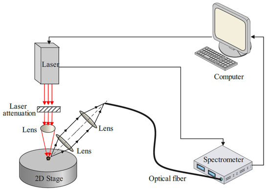
Figure 1.
Diagram of the LIBS system.
2.2. Coal Samples
The 100 coal samples used in this work were from Hebei Province, China. The results of proximate analysis (true value mentioned in this paper) were measured by electric ovens and muffle stoves according to the Chinese national standard (GB/T 212-2008). The proximate analysis of coal was under a dry basis because the moisture of the coal sample is easily affected by the environment, which led to the moisture mismatch between the LIBS spectrum and the original proximate analysis, while the ash, volatile and other results do not change under the drying basis. The specific values are shown in Table A1 in Appendix A.
The coal block was first ground into powders with a diameter of less than 0.2 mm. Then, 0.6 g powder was pressed into a pellet at a pressure of 30 MPa, with a thickness of about 1.3 mm, and a diameter of 2 cm. There were 20 ablation points on each coal pellet, each ablation point was excited 10 times. Thus, 200 (20 × 10) spectra can be obtained for each coal pellet, and the average of 200 spectral intensities is used to represent the LIBS spectrum of the current coal.
3. LIBS Spectral Pretreatment
3.1. Baseline Removal
The baseline of the average spectrum is prone to drift, owing to the disturbance from the environment and equipment, which deteriorates the spectral accuracy and analysis results. Thus, baseline removal is indispensable for the improvement of the signal-to-noise ratio (SNR). Herein, three main baseline removal methods were induced, including the Modpoly method, IModPoly method, and Zhang fit method [18,19,20], and the results are shown in Figure 2. It was indicated that the Zhang fit method could better remove the background noise by using an adaptive iteratively reweighted penalty least squares algorithm (airPLS) [20]. There was no user intervention and prior information, and it depended on the iterative weight change in the squared error between the fitted baseline and the original signal, which runs fast and flexibly.
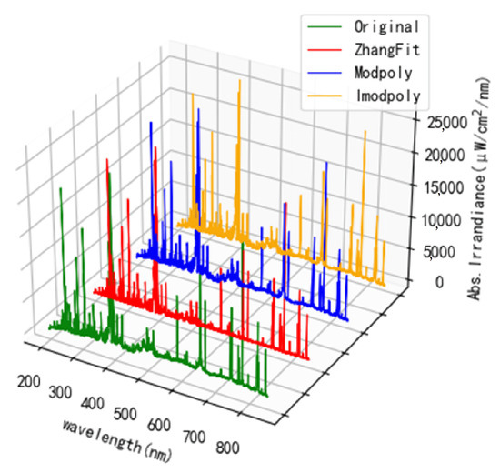
Figure 2.
The performance of different baseline removal methods for LIBS spectra.
3.2. Standardization
The spectral standardization was to normalize the intensity at the same wavelength, which aimed to scale the spectral data to the same level and minimize the data difference. Some machine learning methods rely on the calculation of distance, for example, principal component analysis and K-nearest neighbor, therefore, standardization was necessary. Some methods that prefer data features to conduct might not need to be standardized, such as random forest algorithms. One of the most common standardization methods is Z-scores, which transform the data with normal distribution into a standardized normal distribution. The equation is shown below:
where is the spectral intensity after standardization; is the spectral intensity; μ is the average spectral intensity of all spectra at the current wavelength; and σ is the standard deviation of the spectral intensity of all spectra at the current wavelength.
3.3. Peak Determination
The peaks were first extracted according to the local maximum value of the spectra; however, the peak wavelength may shift from the standard wavelength from the National Institute of Standards and Technology (NIST). Thus, the selected peaks need to be further matched to the atomic spectral wavelength based on the excitation probability and the elements in the coal. The determination of peak wavelength after correction is shown in Figure 3.
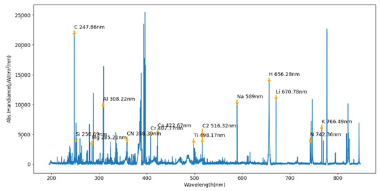
Figure 3.
Schematic of the characteristic peak wavelength position.
Then, some peaks with high intensity and more repetitions were used to perform the classification and quantification work. Because the low-intensity peaks had larger RSD and were considered background radiation, which is not conducive for modeling, thus, the intensity threshold for the baseline removal was set as 2000, and the repetition of peaks was set to 50 to perform the data cleaning. As a result, 54 characteristic peaks were obtained, as shown in Table 1 for details.

Table 1.
Characteristic peaks used in this article for classification and quantification.
3.4. Model Validation
After the collection of LIBS spectra, the database of 100 coal samples was randomly divided into training, test, and prediction sets. The training and test sets consist of 70% (70 samples), and the prediction set accounts for 30% (30 samples). The training set is used for model training, and the test set is used for cross-validation to find out the best performance of the model and avoid overfitting. The prediction set is composed of coal spectra, and the proximate analysis is only used to evaluate the prediction performance instead of model training and validation.
The model validation and parameter selection were realized by cross-validation, which could evaluate the accuracy and robustness of the model and select the optimal parameter for modeling. Herein, the leave-one-out cross-validation (LOOCV) was used for the classification model and five-fold cross-validation was used for the quantification model. These two methods both belong to K-fold cross-validation, which divides the dataset into K parts, of which K − 1 parts are the training set, and the remaining parts are the test set. The difference is that the test set of LOOCV is 1 sample, and the test set of five-fold cross-validation is 14 samples. In addition, each part of the dataset will be as the test set in turn (K times), thus K model validation results can be obtained after the cross-validation. The average value of K model validation results can be considered as the basis for the model tuning.
3.5. Model Indicators
(1) Evaluation indicator of clustering models
The silhouette coefficient is an evaluation indicator for the clustering model. For each sample, the intra-cluster dissimilarity a(i) and the inter-cluster dissimilarity b(i) were calculated to obtain the average silhouette coefficient of the model. The intra-cluster dissimilarity refers to the average dissimilarity between the point and other points in the same group, and a smaller value indicates that the clustering is more reasonable. The inter-cluster dissimilarity refers to the average dissimilarity between the point and other points in different clusters, and a bigger value means that the clustering is more unreasonable. The average silhouette coefficients can be obtained by the calculation results of all points. The formula for calculating the silhouette coefficient of one sample is as Equation (2):
where S(i) close to 1 indicates that the cluster is reasonable; S(i) close to −1 shows that the sample belongs to other clusters; and close to 0 means that the current sample is on the boundary of the two clusters.
(2) Evaluation indicator of the classification models
A confusion matrix can be used to evaluate the performance of the classification model. The results on the diagonal of the matrix are the number of correct results, and the other results are the number of incorrect results, as shown in Figure 4. On this condition, the accuracy can also be calculated according to the results of the confusion matrix in Equation (3):
where TP is the true positive result; FP is the false positive result; TN is the true negative result; and FN is the false negative result.
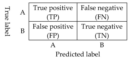
Figure 4.
Schematic diagram of the confusion matrix.
(3) Evaluation indicators of quantification models
The coefficient of determination (R2) describes the fitting degree of the regression model. The closer the R2 is to 1, the better the fitting degree of the model. The other indicator is the root mean square error (RMSE), which can describe the robustness of the model. The closer the RMSE is to 0, the better the stability of the model. For the model validation, the RMSE is the root mean square error of cross-validation (RMSECV), and for the model prediction, the RMSE is the root mean square error of prediction (RMSEP). These two indicators are used to select the optimal parameters for the regression model. Thus, the model parameter with the largest R2 and smallest RMSE should be determined to build the model.
where , , are the true value, average value, and prediction value, respectively, and n and m are the numbers of samples in the test and prediction sets, respectively.
4. Clustering, Classification, and Quantification of Coal Based on Machine Learning
4.1. Clustering Models
Clustering is a type of unsupervised learning method, which extracts the data features only based on the LIBS spectra instead of category labels, including principal component analysis (PCA), K-means clustering, DBSCAN clustering, etc. The spectra in the same cluster are similar, and the spectra between different clusters are significantly different. Thus, the similarity in the same cluster helps understand the property of unknown coal samples, and then the coal information can be roughly characterized.
4.1.1. K-Means Clustering
The K-means clustering divides all samples into K clusters only according to the LIBS spectra. K samples are randomly selected as K initial cluster centers, and then the distance between the first sample that needs to be assigned and each cluster center is calculated, and finally, the sample will be assigned to the closest cluster. Once the first sample is determined, each cluster center will be recalculated until the termination condition is met. The termination condition can be that all samples have been assigned to the cluster center, or the cluster center no longer changes.
The key parameter of the K-means clustering is the K value (number of clusters). The K-means clustering is highly dependent on the initial cluster distribution, which may induce the calculation non-convergence. K values will be determined by the elbow method, and the silhouette coefficient mentioned in Section 3.5 can be used to evaluate the model performance.
The elbow method calculates the sum of the distortion degree for each cluster, where the distortion degree is the sum of the squared distance from each sample point to the clustering center. If the distortion degree is small, the points in the cluster are close to each other; otherwise, the points will be more dispersed. As the K value increases, the number of samples contained in each cluster decreases, and the distortion degree for the cluster becomes smaller. However, when the K value increases to a certain extent, the distortion degree has no obvious improvement. Thus, the elbow point is where the slope suddenly slows down, and the K value can be considered the best parameter under this condition.
The number of input variables of K-means clustering is up to two-dimensional features; thus, the 54 variables mentioned in Section 3.3 are reduced to 2 principal components by PCA. The results of the elbow method under different K values are shown in Figure 5a. When K is equal to 4, the slope of the curve slows down, which can be determined as the elbow point. Hence, coal can be divided into four clusters with totally different LIBS spectra as shown in Figure 5b.
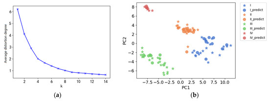
Figure 5.
Elbow rule descent curve for K-means clustering (a) and clustering results for best K values (b).
The results showed that the silhouette coefficient of the training set and the test set was 0.621, and for the prediction set was 0.663. The silhouette coefficient for a dataset is close to 1, which indicated that the results of K-means clustering were reasonable. K-means clustering will be able in the future to estimate the category and the proximate analysis data for an unknown sample based on the LIBS spectra and current database.
4.1.2. DBSCAN Clustering
Density-Based Spatial Clustering of Applications with Noise (DBSCAN) clustering is a density-based method. It first selects a sample point randomly from the dataset and then find out all the available points under the combination of the radius (ε) and the minimum number of neighboring points (minPts). If the sample number in the circle with the radius of ε is higher or equal to the minPts, the circle will be transferred to the next sample points; if the sample point is on the edge of the dataset, the clustering center will be re-selected until an appropriate clustering center appears. There is no limitation for DBSCAN clustering on the shape and number of clusters, and it is not sensitive to anomalous data. However, DBSCAN clustering has some requirements of the data density and sample balance, and different parameters have different results.
The key parameters of DBSCAN clustering are the circle radius (ε) and the minimum number of neighboring points in the circle (minPts). If the circle radius is too large or small, the clustering performance will be poor and unreasonable, and it will generate too few clusters or too many clusters. The minPts value refers to the threshold for the number of samples in the circle, and if the number of samples in the circle is greater than or equal to the threshold, the sample is considered to be the clustering center. The minPts value is usually related to the feature dimension.
Two same principal components were input as the K-means clustering to reduce the dimension. The circle radius ε of the DBSCAN clustering is determined by the elbow point of the k-distance plot, which is the same as K-means clustering. The k-distance values between all sample points were arranged in descending order in the k-distance plot as shown in Figure 6a. Thus, the circle radius ε can be determined as three according to the elbow method. The minPts is usually recommended as the feature dimension multiplied by two, hence, the minPts value is considered to be four. The results of DBSCAN clustering are shown in Figure 6b.
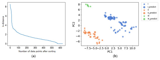
Figure 6.
K-distance plot (a) and clustering results (b) of DBSCAN clustering.
The silhouette coefficient of the training and test sets was 0.604, and the silhouette coefficient of the prediction set was 0.437, lower than the K-means clustering. The low silhouette coefficient of the prediction set is strongly related to poor data density and data imbalance. For example, the number of the sample in the training set is three, which is lower than the minPts value. On this condition, the DBSCAN clustering considered these three samples as noise and then filtered them. Although some imbalanced data were filtered, the remaining results were still meaningful. The results indicated that the 100 coal samples could be split into three different clusters only according to LIBS spectra.
4.2. Classification Models
Classification is a type of supervised learning, which learns the regularity between the LIBS spectra and labels to predict the unknown coal samples, mainly including K-nearest neighbor (KNN), random forest classification (RFC), etc. The classification model can also be used before the establishment of the regression model, because the fitting degree may not be so good for a huge database due to various sub-categories. Thus, the classification model can divide the coal samples into different categories based on the similarity, and then build the regression model within the same categories to obtain a higher fitting degree.
4.2.1. K-Nearest Neighbor
K-nearest neighbor is an instance-based method, and its classification result is obtained by the category of the highest number of near neighbors. The key parameter of the K-nearest neighbor is the K value, which represents the number of observed neighbors and is usually determined by the cross-validation result. If the K value is too small, the model may be overfitting; if the K value is too large, the sample with a further distance may lead to a wrong prediction result. The calculation of distance is based on Euclidean distance, thus, the spectra database needed to be standardized before modeling in case the algorithm attaches more importance to the largest intensity and ignores the smallest intensity.
The intensity of 54 peaks and their sample labels were used for cross-validation, and the model performed best with an accuracy of 0.957 when k was equal to 2, as shown in Figure 7a. The prediction result with an accuracy of 0.933 as shown in Figure 7b. There were two samples in the K category in the confusion matrix that were predicted as the I category, due to their spectral similarity. Although the prediction results might be wrong, the proximate analysis of the I category was similar to the K category. Thus, the proximate analysis result could be referenced on this condition, which indicated the K-nearest neighbor classification still had strong applicability.
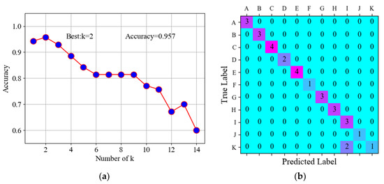
Figure 7.
Cross-validation results (a) and prediction results (b) of K-nearest neighbor classification.
4.2.2. Naive Bayes Classification
Naive Bayes is a type of supervised learning based on the Bayes theorem, which assumes that all the features are independent of each other. Compared with K-nearest neighbor (KNN) and support vector classification (SVC), Naive Bayes learns the relation between features and labels to obtain the distribution probability of features. Then, if the sample spectra are input in the naive Bayes model, the probability of the different labels will be given, and the final prediction result will be the one with the highest probability. Naive Bayes mainly includes Gaussian naive Bayes, polynomial naive Bayes, and Bernoulli distribution naive Bayes. In this work, the Gaussian naive Bayes with simple and lightweight characteristics was adopted, and there was no need for parameter analysis. Thus, the model performance will be evaluated by the confusion matrix of the prediction set.
There is no need for naive Bayes classification to conduct the standardization, and it has a good performance for small-scale data, which can also handle multi-classification tasks. As shown in Figure 8, the confusion matrix showed that only one sample in the F category was predicted as the C category due to the spectral similarity, which was the same condition as the K-nearest neighbor classification mentioned above. The prediction accuracy of naive Bayes was 0.967, which was slightly higher than the K-nearest neighbor.
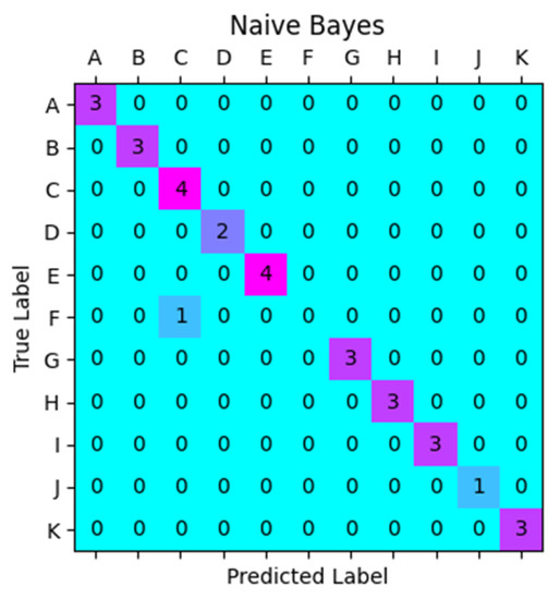
Figure 8.
Prediction results of naive Bayes.
4.3. Regression Models
When the output is no longer labels but continuous variables, the regression model can be used for quantitative analysis. Regression models study the relation between independent variables and dependent variables and then establish a possible function to predict the trend of the dependent variables. The regression model can predict the proximate analysis of coal, such as ash, volatile content, and fixed carbon.
4.3.1. Partial Least Squares Regression
Partial least squares regression (PLSR) is a component variable regression method based on principal component analysis and correlation analysis. The independent variables and dependent variables are projected to a new zone to obtain the principal components, which contain the information of the original data as much as possible. Meanwhile, the PLSR also retains the biggest correlation between independent variables and dependent variables. PLSR is suitable for several situations, for example, multiple independent variables correspond to multiple dependent variables, the independent and dependent variables have strong collinearity, and a small-size database has many independent variables.
The number of partial least squares factors (k) is the key parameter of the PLSR model. The spectral information represented by each partial least squares factor decreases sequentially. If the k value is too big, the PLSR may be overfitting and if the k value is too small, the selected factors may not sufficiently represent the spectral information.
The PLSR model was established for the prediction of ash, volatiles, and fixed carbon, and the cross-validation was conducted by the training and test sets. Then, the maximum R2 value and the minimum RMSECV value were used to determine the best parameters of the model. If these two conditions could not be met at the same time, the condition with the maximum R2 value will be used to build the model, because the RMSECV at this parameter is close to the smallest RMSECV value. Thus, the accuracy and stability of the model are similar to each other.
When the factor k of partial least squares was 12, the R2 value was the largest and the RMSECV value is the smallest, with the values of 0.942 and 1.349%, respectively, as shown in Figure 9a. Then, the spectra of the prediction set were input into the model to obtain the predicted value of ash content. The R2 value and RMSEP for the prediction set were 0.970 and 1.012%, respectively. According to the definition and Equation (6), the RMSEP could be considered as the predicted error.
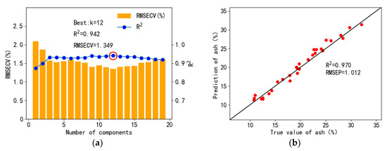
Figure 9.
Cross-validation results of ash quantification with partial least squares regression (a) and prediction set regression results (b).
As for the volatile content, the cross-validation and prediction results are shown in Figure 10. When k was equal to 17, the R2 value was the largest, and the RMSECV value was the smallest, with values of 0.882 and 0.803%, respectively. As for the prediction set, the R2 value and RMSEP were 0.934 and 0.878%, respectively. It was indicated that although the fitting degree of the training set was not so high, the model did not overfit and had good applicability.
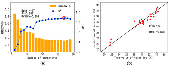
Figure 10.
Cross-validation results of partial least squares regression volatile quantification (a) and prediction set regression results (b).
For the fixed carbon, the cross-validation and prediction results are shown in Figure 11. When k was equal to 7, the R2 value was the biggest, and the RMSECV value was 1.443%; however, the minimum RMSECV value (1.396%) appeared when k was equal to 10. Thus, the differences between these two models were little, k equal to 7 was used for modeling. The R2 value and RMSEP value of the prediction set were 0.956 and 1.409%, respectively. The physical relation of ash, volatile, and fixed carbon meets the sum of 100% on a dry basis, and the cross-validation results and prediction results of the ash and volatile content were good. Thus, the prediction performance of fixed carbon may not greatly deviate. The results showed that both the cross-validation and prediction had good performance on the ash, volatile, and fixed carbon content, which indicated that the selected peaks in Section 3.3 had a good correspondence with the proximate analysis results.
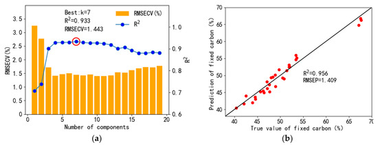
Figure 11.
Cross-validation results of partial least squares regression fixed carbon quantification (a) and prediction set regression results (b).
4.3.2. LASSO Regression
Least absolute convergence and selection operator (LASSO) regression minimize the sum of squared residuals and generate some regression coefficients equal to 0 when the sum of the absolute values of the regression coefficients is less than a constant. LASSO regression can be concluded that L1 regularization is implemented based on the least squares method, which can make the variables sparse to remove some variables that are not conducive to regression. Thus, the remaining variables will play a key role in the regression model. Compared with L1 regularization, L2 regularization (ridge regression) obtained smooth solutions instead of sparse solutions. In other words, the regression coefficients of some dimensions are close to 0 rather than equal to 0, which also simplifies the complexity of the regression model.
The key parameter of LASSO regression is the alpha value, which is the degree that the regression coefficient tends to zero. When alpha is close to zero, the model is the ordinary least squares method solved by linear regression. The alpha values at 0.3, 0.5, and 1.0 were first calculated to find some regularity. The results showed that the fitting degree of the model decreased with the increase in alpha value. Thus, the range of alpha could be determined from 0.01 to 0.4, and each time increased by 0.02 to find the index with the maximum R2 value and minimum RMSECV value.
In general, the performance of PLSR was better than LASSO regression, and the selected parameter was close to 0, which was similar to the ordinary least squares method. Thus, the calculation could be conducted with the assistance of L2 regularization to improve the model accuracy.
The cross-validation and prediction results of the ash LASSO regression were shown in Figure 12. When the alpha was 0.15, the accuracy and stability of the model on the training and test set were the best. For the prediction set, the R2 value was 0.967 and the RMSEP was 1.063%, which was similar to the result of PLSR. Thus, both LASSO regression and PLSR had a good performance to remove collinearity and implement the regression of ash.
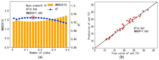
Figure 12.
Cross-validation results (a) and prediction set regression results (b) for LASSO regression ash quantification.
The quantification results for volatiles by using LASSO regression are shown in Figure 13, and the optimal alpha value of the model was 0.01, which indicated that the L1 regularization of the LASSO regression did not play an important role in modeling. LASSO regression performs better in feature selection with high-dimensional data, which indicated more spectral peaks could be introduced for the model training, especially for LASSO regression. The cross-validation R2 was 0.840, RMSECV was 0.923%, prediction R2 was 0.904, and RMSEP was 1.060%, which was inferior to PLSR.
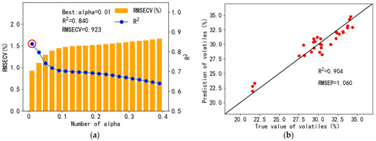
Figure 13.
Cross-validation results (a) and prediction set regression results (b) for LASSO regression volatile quantification.
As shown in Figure 14, when alpha was equal to 0.05, the cross-validation results of fixed carbon were the best, with cross-validation R2 and RMSECV values of 0.942 and 1.310%. On this condition, LASSO regression was similar to the ordinary least squares regression, which also indicated that the PLSR was more applicable than LASSO regression to the current coal database.
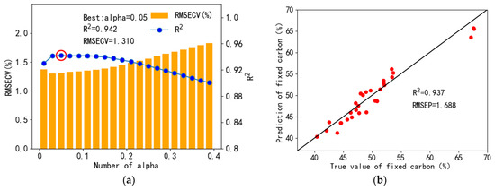
Figure 14.
Cross-validation results of LASSO regression fixed carbon quantification (a), and prediction set regression results (b).
4.4. Performance Comparison
According to the calculation results mentioned in Section 4, the performances of different clustering, classification, and regression model are shown in Table 2, which might provide a reference for the model selection when applying LIBS in the industry. As for the clustering model, the K-means clustering had a better performance than DBSCAN clustering; as for the classification model, the naive Bayes performed better on the prediction set than the K-nearest neighbor; as for the regression model, the PLSR model showed a better result than LASSO regression on the proximate analysis, such as ash, volatiles, and fixed carbon.
Table 2.
The different performances of clustering, classification, and regression models.
5. Conclusions
The existing methods for the detection of coal are labor intensive and time consuming. In this work, LIBS technology assisted with machine learning was introduced to support the current condition that the coal quality information lags in the real-time combustion status in the coal-fired boiler. The experimental optimization was conducted to reduce the spectral RSD, and the pretreatment of LIBS spectra was used for the removal of noise and laid a foundation for classification and qualification. Then, two clustering models, two classification models, and two regression models were established to show their application conditions and performances.
Two clustering models could realize the clustering of coal samples according to the LIBS spectra with unknown labels, and the results showed that K-means clustering could effectively divide coal samples into four clusters that the spectra and coal quality information of samples within the same cluster were similar to each other. As for the two classification models, they could trace the source of coal samples with known labels, and the results indicated that the prediction performance of naive Bayesian classification was better than the K-nearest neighbor with a prediction accuracy of 0.967. Two regression models could give quantitative prediction results of various proximate analysis indicators, the PLSR showed better performance than the LASSO regression, and the RMSEP of ash, volatiles, and fixed carbon were 1.012%, 0.878%, and 1.409%, respectively.
In this work, the performance of different results could provide a reference when applying LIBS to industry. In addition, attention should be paid to the improvement of LIBS spectral accuracy, repeatability, and the fitting degree of classification and regression model. In the future, if the mentioned three factors can be achieved at the same time, meanwhile, there is a similar prediction sample in the database, the prediction accuracy will be perfect, which is also an important development trend in LIBS technology.
Author Contributions
Writing—original draft, Y.Z.; methodology, Q.L.; software, A.C.; writing—review and editing, Y.L.; supervision, X.R. All authors have read and agreed to the published version of the manuscript.
Funding
This research was funded by the Hebei Administration for Market Regulation Science and Technology Program of China, grant number: 2022ZD09.
Institutional Review Board Statement
Not applicable.
Informed Consent Statement
Not applicable.
Data Availability Statement
Not applicable.
Conflicts of Interest
The authors declare no conflict of interest.
Appendix A
Table A1.
Proximate analysis results of 100 coal samples.
Table A1.
Proximate analysis results of 100 coal samples.
| Number | Label * | Ash d ** (%) | Volatiles d (%) | Fixed Carbon d (%) |
|---|---|---|---|---|
| 1 | A | 22.96 | 30.24 | 46.80 |
| 2 | A | 23.03 | 30.47 | 46.50 |
| 3 | A | 22.42 | 30.49 | 47.09 |
| 4 | A | 23.69 | 30.23 | 46.08 |
| 5 | A | 22.65 | 30.17 | 47.18 |
| 6 | A | 23.13 | 30.39 | 46.48 |
| 7 | B | 11.32 | 22.13 | 66.55 |
| 8 | B | 11.38 | 21.97 | 66.65 |
| 9 | B | 11.72 | 21.58 | 66.70 |
| 10 | B | 10.57 | 21.98 | 67.45 |
| 11 | B | 11.04 | 21.83 | 67.13 |
| 12 | B | 10.91 | 21.94 | 67.15 |
| 13 | B | 10.82 | 21.48 | 67.70 |
| 14 | B | 10.75 | 21.58 | 67.67 |
| 15 | B | 10.85 | 21.57 | 67.58 |
| 16 | C | 20.19 | 31.79 | 48.02 |
| 17 | C | 17.86 | 33.21 | 48.93 |
| 18 | C | 19.25 | 32.50 | 48.25 |
| 19 | C | 19.31 | 32.59 | 48.10 |
| 20 | C | 19.73 | 32.66 | 47.61 |
| 21 | C | 19.35 | 32.29 | 48.36 |
| 22 | C | 18.97 | 32.43 | 48.60 |
| 23 | C | 19.66 | 32.40 | 47.94 |
| 24 | C | 18.96 | 32.64 | 48.40 |
| 25 | C | 19.75 | 32.28 | 47.97 |
| 26 | C | 19.08 | 32.19 | 48.73 |
| 27 | D | 22.89 | 29.43 | 47.68 |
| 28 | D | 22.39 | 30.20 | 47.41 |
| 29 | D | 22.96 | 29.70 | 47.34 |
| 30 | D | 24.38 | 29.38 | 46.24 |
| 31 | D | 22.09 | 30.48 | 47.43 |
| 32 | D | 26.16 | 29.29 | 44.55 |
| 33 | D | 21.58 | 30.23 | 48.19 |
| 34 | D | 22.93 | 30.02 | 47.05 |
| 35 | E | 25.04 | 29.86 | 45.10 |
| 36 | E | 25.03 | 30.41 | 44.56 |
| 37 | E | 25.56 | 29.50 | 44.94 |
| 38 | E | 24.08 | 30.26 | 45.66 |
| 39 | E | 25.80 | 29.98 | 44.22 |
| 40 | E | 28.22 | 29.90 | 41.88 |
| 41 | E | 27.02 | 29.57 | 43.41 |
| 42 | E | 27.94 | 28.11 | 43.95 |
| 43 | E | 24.98 | 29.93 | 45.09 |
| 44 | E | 26.04 | 29.44 | 44.52 |
| 45 | E | 25.98 | 29.90 | 44.12 |
| 46 | F | 16.64 | 31.82 | 51.54 |
| 47 | F | 16.63 | 31.50 | 51.87 |
| 48 | F | 16.47 | 31.59 | 51.94 |
| 49 | F | 16.20 | 31.91 | 51.89 |
| 50 | F | 15.42 | 32.08 | 52.50 |
| 51 | G | 19.55 | 30.06 | 50.39 |
| 52 | G | 17.82 | 31.05 | 51.13 |
| 53 | G | 19.50 | 30.71 | 49.79 |
| 54 | G | 21.47 | 29.58 | 48.95 |
| 55 | G | 19.21 | 30.30 | 50.49 |
| 56 | G | 23.16 | 29.53 | 47.31 |
| 57 | G | 20.26 | 30.29 | 49.45 |
| 58 | G | 21.83 | 29.61 | 48.56 |
| 59 | G | 23.74 | 28.92 | 47.34 |
| 60 | G | 21.79 | 30.24 | 47.97 |
| 61 | G | 19.29 | 29.88 | 50.83 |
| 62 | H | 30.31 | 28.15 | 41.54 |
| 63 | H | 32.07 | 27.52 | 40.41 |
| 64 | H | 32.07 | 27.55 | 40.38 |
| 65 | H | 31.52 | 27.12 | 41.36 |
| 66 | H | 31.76 | 28.48 | 39.76 |
| 67 | H | 30.85 | 28.26 | 40.89 |
| 68 | H | 28.43 | 29.24 | 42.33 |
| 69 | H | 34.54 | 26.84 | 38.62 |
| 70 | H | 30.96 | 27.63 | 41.41 |
| 71 | H | 28.36 | 29.12 | 42.52 |
| 72 | H | 29.70 | 28.24 | 42.06 |
| 73 | I | 11.29 | 34.71 | 54.00 |
| 74 | I | 11.96 | 34.64 | 53.40 |
| 75 | I | 11.34 | 35.06 | 53.60 |
| 76 | I | 11.85 | 33.89 | 54.26 |
| 77 | I | 12.22 | 34.39 | 53.39 |
| 78 | I | 11.90 | 34.62 | 53.48 |
| 79 | I | 10.45 | 34.73 | 54.82 |
| 80 | I | 13.10 | 33.89 | 53.01 |
| 81 | I | 12.54 | 34.01 | 53.45 |
| 82 | I | 12.56 | 33.80 | 53.64 |
| 83 | J | 18.71 | 32.12 | 49.17 |
| 84 | J | 17.66 | 32.28 | 50.06 |
| 85 | J | 15.92 | 32.90 | 51.18 |
| 86 | J | 17.89 | 32.38 | 49.73 |
| 87 | J | 20.63 | 31.35 | 48.02 |
| 88 | J | 19.66 | 31.44 | 48.90 |
| 89 | J | 17.37 | 32.56 | 50.07 |
| 90 | J | 17.34 | 31.26 | 51.40 |
| 91 | J | 19.87 | 31.49 | 48.64 |
| 92 | J | 17.78 | 31.51 | 50.71 |
| 93 | K | 13.96 | 33.57 | 52.47 |
| 94 | K | 15.03 | 33.50 | 51.47 |
| 95 | K | 15.72 | 33.25 | 51.03 |
| 96 | K | 14.31 | 33.75 | 51.94 |
| 97 | K | 15.42 | 33.18 | 51.40 |
| 98 | K | 13.73 | 34.18 | 52.09 |
| 99 | K | 13.86 | 33.88 | 52.26 |
| 100 | K | 16.34 | 33.12 | 50.54 |
* The label was determined by the origin of coal. ** Dry basis.
References
- Charbucinski, J.; Nichols, W. Application of spectrometric nuclear borehole logging for reserves estimation and mine planning at Callide coalfields open-cut mine. Appl. Energy 2003, 74, 313–322. [Google Scholar] [CrossRef]
- Parus, J.; Kierzek, J.; Malozewska-Bucko, B. Determination of the carbon content in coal and ash by XRF. X-ray Spectrom. 2000, 29, 192–195. [Google Scholar] [CrossRef]
- Ctvrtnickova, T.; Mateo, M.P.; Yanez, A.; Nicolas, G. Application of LIBS and TMA for the determination of combustion predictive indices of coals and coal blends. Appl. Surf. Sci. 2011, 257, 5447–5451. [Google Scholar] [CrossRef]
- Senesi, G.S.; Senesi, N. Laser-induced breakdown spectroscopy (LIBS) to measure quantitatively soil carbon with emphasis on soil organic carbon. A review. Anal. Chim. Acta 2016, 938, 7–17. [Google Scholar] [CrossRef] [PubMed]
- Harmon, R.S.; Remus, J.; McMillan, N.J.; McManus, C.; Collins, L.; Gottfried, J.L.; DeLucia, F.C.; Miziolek, A.W. LIBS analysis of geomaterials: Geochemical fingerprinting for the rapid analysis and discrimination of minerals. Appl. Geochem. 2009, 24, 1125–1141. [Google Scholar] [CrossRef]
- Sezer, B.; Bilge, G.; Boyaci, I.H. Capabilities and limitations of LIBS in food analysis. TrAC-Trends Anal. Chem. 2017, 97, 345–353. [Google Scholar] [CrossRef]
- de Carvalho, G.G.A.; Guerra, M.B.B.; Adame, A.; Nomura, C.S.; Oliveira, P.V.; de Carvalho, H.W.P.; Santos, D.; Nunes, L.C.; Krug, F.J. Recent advances in LIBS and XRF for the analysis of plants. J. Anal. At. Spectrom. 2018, 33, 919–944. [Google Scholar] [CrossRef]
- Zhang, H.; Yueh, F.Y.; Singh, J.P.; Cook, R.L.; Loge, G.W. Laser-induced breakdown spectroscopy in a metal-seeded flame. In Collection of Technical Papers, Proceedings of the 35th Intersociety Energy Conversion Engineering Conference and Exhibit (IECEC)(Cat. No. 00CH37022), Las Vegas, NV, USA, 24–28 July 2000; IEEE: New York, NY, USA, 2000; Volume 1, pp. 595–600. [Google Scholar]
- Li, W.; Dong, M.; Lu, S.; Li, S.; Wei, L.; Huang, J.; Lu, J. Improved measurement of the calorific value of pulverized coal particle flow by laser-induced breakdown spectroscopy (LIBS). Anal. Methods 2019, 11, 4471–4480. [Google Scholar] [CrossRef]
- Yu, Z.; Yao, S.; Jiang, Y.; Chen, W.; Xu, S.; Qin, H.; Lu, Z.; Lu, J. Comparison of the matrix effect in laser induced breakdown spectroscopy analysis of coal particle flow and coal pellets. J. Anal. At. Spectrom. 2021, 36, 2473–2479. [Google Scholar] [CrossRef]
- Feng, J.; Wang, Z.; West, L.; Li, Z.; Ni, W. A PLS model based on dominant factor for coal analysis using laser-induced breakdown spectroscopy. Anal. Bioanal. Chem. 2011, 400, 3261–3271. [Google Scholar] [CrossRef] [PubMed]
- Yao, S.; Mo, J.; Zhao, J.; Li, Y.; Zhang, X.; Lu, W.; Lu, Z. Development of a Rapid Coal Analyzer Using Laser-Induced Breakdown Spectroscopy (LIBS). Appl. Spectrosc. 2018, 72, 1225–1233. [Google Scholar] [CrossRef] [PubMed]
- Qin, H.; Lu, Z.; Yao, S.; Li, Z.; Lu, J. Combining laser-induced breakdown spectroscopy and Fourier-transform infrared spectroscopy for the analysis of coal properties. J. Anal. At. Spectrom. 2019, 34, 347–355. [Google Scholar] [CrossRef]
- Li, L.-N.; Liu, X.-F.; Yang, F.; Xu, W.-M.; Wang, J.-Y.; Shu, R. A review of artificial neural network based chemometrics applied in laser-induced breakdown spectroscopy analysis. Spectrochim. Acta. Part B At. Spectrosc. 2021, 180, 106183. [Google Scholar] [CrossRef]
- Brunnbauer, L.; Gajarska, Z.; Lohninger, H.; Limbeck, A. A critical review of recent trends in sample classification using Laser-Induced Breakdown Spectroscopy (LIBS). TrAC Trends Anal. Chem. 2023, 159, 116859. [Google Scholar] [CrossRef]
- Dong, M.; Wei, L.; González, J.J.; Oropeza, D.; Chirinos, J.; Mao, X.; Lu, J.; Russo, R.E. Coal Discrimination Analysis Using Tandem Laser-Induced Breakdown Spectroscopy and Laser Ablation Inductively Coupled Plasma Time-of-Flight Mass Spectrometry. Anal. Chem. 2020, 92, 7003–7010. [Google Scholar] [CrossRef] [PubMed]
- Zhang, Y.; Xiong, Z.; Ma, Y.; Zhu, C.; Zhou, R.; Li, X.; Li, Q.; Zeng, Q. Quantitative analysis of coal quality by laser-induced breakdown spectroscopy assisted with different chemometric methods. Anal. Methods 2020, 12, 353–3536. [Google Scholar] [CrossRef] [PubMed]
- Lieber, C.A.; Mahadevan-Jansen, A. Automated Method for Subtraction of Fluorescence from Biological Raman Spectra. Appl. Spectrosc. 2003, 57, 1363–1367. [Google Scholar] [CrossRef] [PubMed]
- Zhao, J.; Lui, H.; McLean, D.I.; Zeng, H. Automated Autofluorescence Background Subtraction Algorithm for Biomedical Raman Spectroscopy. Appl. Spectrosc. 2007, 61, 1225–1232. [Google Scholar] [CrossRef] [PubMed]
- Zhang, Z.-M.; Chen, S.; Liang, Y.-Z. Baseline correction using adaptive iteratively reweighted penalized least squares. Analyst 2010, 135, 1138–1146. [Google Scholar] [CrossRef] [PubMed]
Disclaimer/Publisher’s Note: The statements, opinions and data contained in all publications are solely those of the individual author(s) and contributor(s) and not of MDPI and/or the editor(s). MDPI and/or the editor(s) disclaim responsibility for any injury to people or property resulting from any ideas, methods, instructions or products referred to in the content. |
© 2023 by the authors. Licensee MDPI, Basel, Switzerland. This article is an open access article distributed under the terms and conditions of the Creative Commons Attribution (CC BY) license (https://creativecommons.org/licenses/by/4.0/).