Decreasing the Rail Potential of High-Speed Railways Using Ground Wires

Featured Application

This work belongs to the field of railway electrification engineering. The results have certain reference value for reducing the rail potential to ensure the safe operation of electrified railways.

Abstract

For high-speed railways, the rail potential, i.e., the electrical potential difference between the rail and the ground, can be considerably higher than that of conventional speed electric railways and become a safety risk to the signaling devices along the line, because of the large train currents and the high rail–ground leakage resistance. Proper countermeasures must be taken to decrease the rail potential to a safe level. This paper first provides a brief theoretical discussion of the principles of how the rail potential arises and how to suppress it. Then, a program, TRANAS, that was developed for traction network analysis is used to calculate the effects of various suppression countermeasures for an AT feeding system, which include cross-bonding of tracks, inserting CPWs, grounding using catenary masts, laying bare buried ground wires and connecting to dedicated grounding grids, which are evaluated based on the calculation results. The use of buried ground wires shows good prospects for solving electric safety problems in an integrated way, which is investigated in detail. The fact that GWs can suppress the rail potential is attributed to the decrease in the leakage resistance of the return circuit, meaning a relatively small cross-section will be enough for them.

1. Introduction

In electrified railways, the rail not only serves as the running track of the train but also participates in the overall process of traction return current flow. Strictly speaking, it is not a simple grounding conductor, and the connection between the rail and the ground is not completely insulated. Instead, there is leakage conductivity that causes some of the current on the rail to flow into the ground [1]. Then, the current returns back to the rail in places near the substation and return point. The maximum value of the rail potential, which may cause a series of hazards to railway system operation, arises at the position where the train runs and at other positions where the current returns [2]. In the electrical discipline, the rail potential can be reduced by increasing the rail–ground leakage conductance [3]. However, in the signal discipline, in order to ensure the reliable operation of the signal track circuit, the ground leakage conductance should be as small as possible. From this point of view, understanding how to better cooperate between railway electrification engineering and railway signaling engineering is also a key issue in the study of ground return [4].

As an important path for traction return, the rail should have its potential within a safe range guaranteeing the safety of train operation [5]. Generally, a high-power traction load, i.e., a high-power electric locomotive, absorbs a large traction current from the traction network, which in turn leads to a large rail return current [6,7]. Furthermore, under the condition of a high driving density, a great amount of rail current will be formed by the superposition of multi-locomotive currents, resulting in a high rail potential. It is necessary to take certain measures to reasonably control the distribution of the rail potential and rail current, preventing a large step voltage and contact voltage, and ensuring the safe and reliable operation of electrified railway systems [8,9].

Although China’s railway development began later than that of other countries, China has gradually become the country with the highest high-speed railway mileage in the world. High-speed railways have the characteristics of a large traction current, large rail leakage resistance, etc. It is necessary to constantly improve the problems existing in the traction return system to adapt to the development of railway systems [10]. For the distribution problem of traction return flow, ref. [11] mainly studied the influence of the wire diameters of different through-ground wires on the distribution of traction return current proportions and analyzed the current proportion distributed by each wire in the return current path through modeling. Reference [12] focused on the increase in the rail current and potential, analyzing the distribution of the traction current in the track.

France, Germany and Japan are countries that developed their high-speed railways earlier and are typical representatives of advanced railway electrification technology [13,14]. The grounding mode of French railway lines is direct grounding with integrated ground wires. The return process is completed jointly by rails, return wires, ground wires and choke coils. Equipotential bonding is achieved through the full transverse connection of longitudinal conductors. The full transverse connection distance between two track circuits is generally not less than 1 km, which is also convenient for rail break inspection. German railways also adopt the direct grounding mode, with integrated ground wires. The equipotential bonding line, rail and return line of each longitudinal conductor complete the return process together. The rail has longitudinal and horizontal electrical connections. In order to obtain a smooth return path and ensure the normal operation of the track circuit, the conductor in the integrated earthing system is grounded and connected to a grounding strip. The grounding system of the Japanese railway has the functions of lightning protection and reducing electromagnetic induction. The grounding types include lightning rod and arrester grounding, and working grounding. Devices are installed in Japanese stations to prevent excessive rail potential, which can be achieved through the equipotential bonding of up and down rails and decentralized grounding of rails to ensure the normal operation of the return current system. References [15,16] utilized Matlab/Simulink to run a rail potential model of a railway system and compared the effects of different amounts of leakage conductance on the distribution of the rail potential. Reference [17] analyzed the influence on the rail potential distribution by changing the potential partition coefficient of high-speed railway rails.

The rail potential problem has a very long research history [18]. For high-speed railways, due to the heavy loads, large short-circuit currents and high rail–ground leakage resistance, the rail potential can be considerably higher than that of conventional speed electric railways. High-speed railways normally adopt a 2 × 25 kV auto-transformer (AT) power feeding system, whose traction network is of a multi-mesh type. For Chinese high-speed railways, the traction current return configuration and grounding system are similar to those used in France. However, the OCS structure in China mainly adopts a stitched simple catenary with larger tensions of the contact and messenger wires. To obtain the rail potential distribution, one must look to computer simulation programs. In this paper, firstly, a brief theoretical review of the rail potential problem is provided, and then a simulation program, TRANAS, is introduced. Some calculation results are presented, which are used to evaluate the effects of various suppression countermeasures including cross-bonding of tracks, inserting CPWs, grounding using catenary masts, laying bare buried ground wires and connecting to dedicated grounding grids.

2. Theoretical Review

The rail and the ground are not well insulated, nor do they have an ideal metallic contact. When currents propagate along the rail, rail potentials are produced due to the existence of rail–ground leakage resistance. See the simple T–R feeding system shown in Figure 1.

For 0 < x < l, we have

$$\left\{\begin{array}{l}-\frac{d{V}_2(x)}{dx}=Z_{22}{I}_2(x)+Z_1{}_2{I}_1\hfill \\ -\frac{d{I}_2(x)}{dx}=Y{V}_2(x)\hfill \end{array}\right.$$

(1)

and for x < 0 or x > l, we have

$$\left\{\begin{array}{l}-\frac{d{V}_2(x)}{dx}=Z_{22}{I}_2(x)\hfill \\ -\frac{d{I}_2(x)}{dx}=Y{V}_2(x)\hfill \end{array}\right.$$

(2)

where V₂(x) and I₂(x) are the rail potential and current at x km with the units V and A, respectively; Z₂₂ and Z₁₂ are the rail impedance and mutual impedance between the rail and OCS with the common unit Ω/km; Y = 1/R_g is the rail–ground leakage conductance with the unit S/km; and R_g is the rail–ground leakage resistance with the unit Ω·km.

The rail current and potential can be solved as

$$I_2(x)=\left\{\begin{array}{l}\frac{1-n}{2}{I}_1(e^{\gamma x}-e^{-\gamma (l-x)}) (x<0)\hfill \\ -\frac{1-n}{2}{I}_1(e^{-\gamma x}+e^{-\gamma (l-x)})-n{I}_1 (0<x<l)\hfill \\ \frac{1-n}{2}{I}_1(-e^{-\gamma x}+e^{\gamma (l-x)}) (x>l)\hfill \end{array}\right.$$

(3)

$$V_2(x)=\left\{\begin{array}{l}-\frac{1-n}{2}{Z}_0{I}_1(e^{\gamma x}-e^{-\gamma (l-x)}) (x\le 0)\hfill \\ -\frac{1-n}{2}{Z}_0{I}_1(e^{-\gamma x}-e^{-\gamma (l-x)}) (0\le x\le l)\hfill \\ \frac{1-n}{2}{Z}_0{I}_1(-e^{-\gamma x}+e^{\gamma (l-x)}) (x\ge l)\hfill \end{array}\right.$$

(4)

where $\gamma =\sqrt{Z_{22}Y}$ and $Z_0=\sqrt{Z_{22}/Y}$ are the propagation constant and characteristic impedance of the rail with the units 1/km and Ω, respectively, and $n=Z_{12}/Z_{22}$.

At the point where concentrated currents are injected in or drawn out, a jump arises in the rail current, but the distribution of potential along the rail is continuous. The amplitude and phase (in Figure 1, the phase relation is hinted by the polarity) of the rail current and potential vary with the position.

The maximum rail potential takes place at the interfaces of the train and substation, which is

$$V_{2\max }\approx \frac{1-n}{2}{Z}_0{I}_1$$

(5)

Suppose that l is long enough. Equation (5) reveals that the rail potential is in proportion to the rail characteristic impedance and is influenced by the degree of coupling between the rail and OCS.

For booster transformers, auto-transformers or coaxial cable power feeding systems, there will be more concentrative current points on the rail, and the electromagnetic coupling between the rail and other conductors will be more complex. Theoretically, as long as the current loops are identified, the distribution of the rail current and potential can be obtained through the principle of superposition. In fact, practical traction networks are normally more complex than the network shown in Figure 1. The use of a simulation program (validated by measurements) seems necessary to obtain reliable solutions for the rail potential.

3. Rail Potential Problem in High-Speed Railways

3.1. Characteristics

High-speed railways are different from conventional speed railways in the following aspects:

• Large train current. In a 350 km/h EMU with 16 cars, the peak current of the train can exceed 800 A, which is about twice the current of the most powerful electric locomotive.
• Large short-circuit current in traction networks. In China, most substations of high-speed railways obtain electric power from 220 kV grids, which normally have a high short-circuit level. When a fault takes place near the substation, the short-circuit current will be limited only by the impedance of the traction transformer. For a 63 MVA single-phase transformer with a 10.5% impedance, this current will reach up to 20 kA.
• High rail–ground leakage resistance. High-speed railways mainly adopt a ballastless track, which normally has high rail–ground leakage resistance. As an example, in terms of the Japanese material, a value of 100~500 Ω·km has been reported for the Shinkansen, compared to 2~5 Ω·km for normal lines [19].

These factors will lead to high rail potentials in high-speed railways, which may become a danger to the passengers and maintenance personnel and can influence the operation of the signal equipment. Therefore, technical countermeasures must be taken to suppress the rail potentials in high-speed railways.

3.2. Possible Solutions

According to Equation (5), to reduce the rail potential, we must take measures to decrease the rail characteristic impedance and/or to increase the coupling between the rail and OCS. This conclusion can be generalized further in order to include AT, BT and T–R+NF power supply systems. The rail can be viewed as a portion of the return circuit. The return circuit may include other conductors, such as a PW and NF. Therefore, the theoretical measures to suppress rail potentials are as follows: (1) to decrease the longitudinal serial impedance of the return circuit; (2) to increase the transversal shunt conductance of the return circuit; (3) to enhance the electromagnetic coupling between the supply circuit and the return circuit. It is clear that the existence of a PW in AT and an NF in T–R+NF feeding systems can bring the virtues of (1) and (3).

For PDL AT supply systems, the following technical countermeasures can be taken to suppress the rail potentials:

• Bonding the rails of different tracks sufficiently.
• Increasing the connections between the rail and PW (called CPW in some studies).
• Grounding the PW using OCS post foundations.
• Laying one or two directly buried bare wires, which are adequately connected to the rail and PW.
• Utilizing the foundation grounding resistance of various structures along the railway.
• Constructing a special grounding pole along the railway.

Since the rail is also used by railway signal systems, the connection and grounding of the rail must be designed carefully. Normally, planning the traction return circuit should conform to the demands of the signal system to obtain a good EMC on track. Due to the limitation of the interval of signal track circuits, an additional buried bare wire seems a promising solution.

4. Electric Parameter Calculation

This section presents the parameter calculation methods for modeling the traction network. Note that all the theories are coded in a simulation program, named TRANAS (traction network analysis), which was developed in China at the School of Electrical Engineering, Beijing Jiaotong University, Beijing (http://www.bjtuqygds.cn/NewsDetail.aspx?ID=190 (accessed on 28 June 2023)), adopting a node admittance matrix to describe the T–R, T–R+NF, AT, BT and CC traction networks [20,21,22]. Different types of traction power supply systems can, in fact, be modeled uniformly by a chain network that is composed of longitudinal serial elements and transversal shunt elements. A power flow algorithm is introduced, which allows for modeling the train as a PQ load or Iθ load.

4.1. Calculation of Conductor Internal Impedance

For standard copper wire, copper alloy stranded wire, aluminum stranded wire and aluminum alloy stranded wire, the internal impedance calculation is equivalent to that of a cylindrical conductor. The internal impedance of a cylindrical conductor can be expressed by the Kelvin function:

$$Z=\frac{jm\rho }{2\pi r}\frac{\mathrm{ber}(mr)+\mathrm{jbei}(mr)}{\mathrm{ber}\prime (mr)+\mathrm{jbei}\prime (mr)} (\mathrm{\Omega }/\mathrm{m})$$

(6)

where $m=\sqrt{\frac{\omega \mu }{\rho }}$; $\mu ={\mu }_r{\mu }_0$ is the permeability of the conductor; μ₀ = 4π × 10⁻⁷ T·m/A is the permeability of the vacuum; ${\mu }_r$ is the relative permeability (for a non-ferromagnetic conductor, generally, $\mu ={\mu }_0$); $\rho$ and $r$ are the resistivity and radius of the conductor, respectively; and ω is the angle frequency in rad/s.

For steel-core aluminum stranded wire, the calculation of the internal impedance is equivalent to that of a tubular circular conductor. For tubular circular conductors, when the current returns from a distance outside the conductor (the proximity effect can be ignored), the internal impedance calculation formula can be represented by the Kelvin function as

$$Z=\frac{jm\rho }{2\pi r}\frac{(\mathrm{ber}(mr)+\mathrm{jbei}(mr))-\frac{\mathrm{ber}\prime (mq)+\mathrm{jbei}\prime (mq)}{\ker \prime (mq)+\mathrm{jkei}\prime (mq)}(\ker (mr)+\mathrm{jkei}(mr))}{(\mathrm{ber}\prime (mr)+\mathrm{jbei}\prime (mr))-\frac{\mathrm{ber}\prime (mq)+\mathrm{jbei}\prime (mq)}{\ker \prime (mq)+\mathrm{jkei}\prime (mq)}(\ker \prime (mr)+\mathrm{jkei}\prime (mr))} (\mathrm{\Omega }/\mathrm{m})$$

(7)

where $r$ and $q$ are the outer and inner radii of the tubular circular conductor. A solid circular conductor can be regarded as a special case of tubular circular conductor when q = 0. In this case, Equation (7) degenerates into Equation (6). The calculation of the Kelvin functions of ber, bei, ker and kei involved in the formula above can be found in [23].

For contact wires with irregular cross-sections, the influence of the cross-section shape on the effective resistance should be considered when calculating their internal impedance, especially when the concerned harmonic frequency is high. The equivalent radius $r$ of the contact wire can be calculated as

$$r=r_p-(r_p-r_a)e^{-{(\frac{r_p}{15\delta })}^3}$$

(8)

where $r_p$ and $r_a$ are the radii obtained based on an equal perimeter and equal area of the conductor cross-section, respectively, and $\delta$ is the penetration depth.

4.2. Calculation of Impedance of Overhead Conductor–Earth Circuit

The calculation of the external impedance of the overhead conductor–earth circuit (see Figure 2) can be carried out using the Carson–Pollaczek formula [24,25]. The calculation formulas for the external impedance of a single conductor–earth circuit and the mutual impedance of two single conductor–earth circuits are

$$Z_s=\frac{j\omega {\mu }_0}{2\pi }\left(\ln \frac{2h_i}{r_i}+{\displaystyle \underset{0}{\overset{\infty }{\int }}\frac{2e^{-2\lambda h_i}}{\lambda +\sqrt{{\lambda }^2+\frac{j\omega {\mu }_0}{\rho }}}d\lambda }\right)$$

(9)

$$Z_m=\frac{j\omega {\mu }_0}{2\pi }\left[\ln \frac{D_{ik}}{d_{ik}}+{\displaystyle \underset{0}{\overset{\infty }{\int }}\frac{2e^{-\lambda (h_i+h_k)}\cos \lambda x_{ik}}{\lambda +\sqrt{{\lambda }^2+\frac{j\omega {\mu }_0}{\rho }}}d\lambda }\right]$$

(10)

The integral terms of Equations (9) and (10) reflect the influence of finite earth conductivity on impedance, commonly referred to as Carson correction terms, which can be represented by the second type of Bessel function and Struve function. After considering the impedance inside the wire, Dommel organized the above formula as [26]

$$Z_{ii}=(R_{i,\mathrm{int}}+\mathsf{\Delta }{R}_{ii})+j(\frac{\omega {\mu }_0}{2\pi }\ln \frac{2h_i}{r_i}+X_{i,\mathrm{int}}+\mathsf{\Delta }{X}_{ii})$$

(11)

$$Z_{ik}=\mathsf{\Delta }{R}_{ik}+j(\frac{\omega {\mu }_0}{2\pi }\ln \frac{D_{ik}}{d_{ik}}+\mathsf{\Delta }{X}_{ik})$$

(12)

where $Z_{i,\mathrm{i}\mathrm{n}\mathrm{t}}$, $R_{i,\mathrm{i}\mathrm{n}\mathrm{t}}$, $X_{i,\mathrm{i}\mathrm{n}\mathrm{t}}$ and $r_i$ are the internal impedance, ac resistance, internal reactance and radius of the conductor I; $h_i$ and $h_j$ are the average heights from the ground of conductors i and j, respectively; $x_{ik}$, $d_{ik}=\sqrt{{(h_i-h_j)}^2+x_{ik}^2}$ and $D_{ik}=\sqrt{{(h_i+h_j)}^2+x_{ik}^2}$ represent the horizontal distance, distance and mirror distance between conductors i and k, respectively; $\mathsf{\Delta }R$ and $\mathsf{\Delta }X$ are the Carson corrections considering the earth return effect.

For the fundamental frequency, by simplifying $\mathsf{\Delta }R$ and $\mathsf{\Delta }X$, generally used simplified Carson formulas are obtained

$$Z_{ii}=Z_{i,\mathrm{int}}+\frac{\omega {\mu }_0}{8}+j\frac{\omega {\mu }_0}{2\pi }\ln \frac{D_g}{r_i}$$

(13)

$$Z_{ik}=\frac{\omega {\mu }_0}{8}+j\frac{\omega {\mu }_0}{2\pi }\ln \frac{D_g}{d_{ik}}$$

(14)

where $D_g=659\sqrt{\frac{\rho }{f}}$ is the equivalent depth of the earth contour loop.

4.3. Electric Parameters of Directly Buried Ground Wires

The impedance of overhead conductors can be calculated using the Carson–Pollaczek formulas [24]. But for directly buried bare wires (see Figure 3), new formulas must be adopted. In TRANAS, the following equations are introduced [20]. The self-impedance and self-admittance of a directly buried bare wire can be calculated iteratively using Equations (15)–(17):

$$Z(\mathrm{\Gamma })=Z_{\mathrm{int}}+\frac{j\omega {\mu }_0}{2\pi }\ln \frac{1.851}{\sqrt{r^2+4x^2}\sqrt{j\omega {\mu }_0(\frac{1}{\rho }+j\omega {\epsilon }_0)+{\mathrm{\Gamma }}^2}}$$

(15)

$$Y(\mathrm{\Gamma })={\left(\frac{\rho }{\pi }\ln \frac{1.123}{\mathrm{\Gamma }\sqrt{2r\left|x\right|}}\right)}^{-1}$$

(16)

$$\mathrm{\Gamma }=\sqrt{ZY}$$

(17)

where Z_int is the internal impedance of the conductor with the unit Ω/m; x and r represent the height and radius of the conductor with the unit m (x < 0 m for buried wires); ρ and Γ are the earth resistivity and propagation constant with the units Ω·m and 1/m, respectively; ε₀ ≈ 8.854187817 × 10⁻¹² F/m is the permittivity of the vacuum.

These equations were derived from [27,28]. Interestingly enough, different authors seem to provide different illustrations of Sunde’s result. The mutual impedance and mutual potential coefficient of two directly buried bare wires are calculated using

$$Z_{ij}=\frac{j\omega {\mu }_0}{2\pi }\ln \frac{1.851}{d_{ij}\sqrt{j\omega {\mu }_0(\frac{1}{\rho }+j\omega {\epsilon }_0)+{\mathrm{\Gamma }}_i{\mathrm{\Gamma }}_j}}$$

(18)

$$W_{ij}=\frac{\rho }{\pi }\ln \frac{1.123}{\sqrt{d_{ij}{D}_{ij}}\sqrt{{\mathrm{\Gamma }}_i{\mathrm{\Gamma }}_j}}$$

(19)

The mutual impedance between a directly buried wire and an overhead wire is computed using

$$Z_{ik}=\frac{j\omega {\mu }_0}{2\pi }\left[\ln \frac{1.851}{d_{ik}\sqrt{j\omega {\mu }_0(\frac{1}{\rho }+j\omega {\epsilon }_0)+{\mathrm{\Gamma }}^2}}+\frac{2}{3}\sqrt{j\omega {\mu }_0(\frac{1}{\rho }+j\omega {\epsilon }_0)}\left(x_i+x_k\right)\right]$$

(20)

4.4. Theory of Multiconductor Transmission Lines

By treating a uniform multiconductor transmission line as a composite two-port network and using an accurate equivalent π model of the multiphase transmission line, the potential and current on one side can be calculated from the node potential and node injection current on the other side. That is, if the voltage and current vectors at 0 are known, the voltage and current vectors at x can be calculated:

$$\left[\begin{array}{c}V(x)\\ I(x)\end{array}\right]=\left[\begin{array}{cc}\cosh (\sqrt{ZY}x)& \sinh (\sqrt{ZY}x){(ZY)}^{-\frac{1}{2}}Z\\ Y{(ZY)}^{-\frac{1}{2}}\sinh (\sqrt{ZY}x)& \cosh (\sqrt{YZ}x)\end{array}\right]\left[\begin{array}{c}V(0)\\ I(0)\end{array}\right]$$

(21)

where Z and Y are the series impedance matrix and parallel admittance matrix of the traction network.

5. Results

A traction network model was built in the simulation software TRANAS v1.0 according to the methodologies presented in the previous sections. A series of results are presented in this section.

5.1. Network Conditions

Take the AT circuit shown in Figure 4 as the basis, which has the following conditions:

• Two equal AT sections with a 15 km interval;
• A 55 kV source with a 10,000 MVA short-circuit level;
• A 90 MVA single-phase transformer with a 10.5 percent impedance;
• AT leakage impedance of 0.1 + j0.45 Ω;
• Substation and section post grounding resistance of 0.5 Ω;
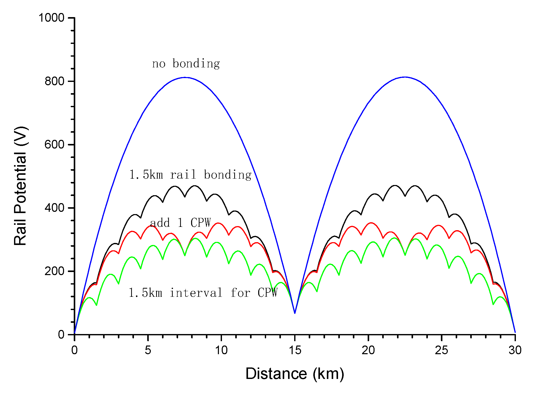
• Interval of 1.5 km for the cross-bonding of two track rails;
• Rail–ground leakage resistance of 100 Ω·km;
• Earth resistivity of 100 Ω·m;
• A PW insulated with an OCS post (see Figure 5 for OCS conductors);
• Train current of 1000 A with a power factor of 0.97.

Figure 4. Basic circuit of the calculated AT network.

Figure 4. Basic circuit of the calculated AT network.

Figure 5. Conductor parameters.

Figure 5. Conductor parameters.

In the following calculations, in order to verify the effects of different countermeasures, some conditions will vary accordingly.

5.2. Effect of Bonding

Figure 6 shows the value of the rail potential at the train position with a 1000 A load current scan from 0 to 30 km.

5.3. Rail–Ground Leakage Resistance

Figure 7 shows the profile of the rail potential when the train is at the 20.25 km position with different values of the rail–ground leakage resistance (R_g).

5.4. OCS Post Resistance

This section considers the scenario where the PW is installed without insulation with an OCS post. Figure 8 shows the profile of the rail potential when the train is at the 20.25 km position with different values of the post grounding resistance (R_p), considering a 60 m span between two adjacent posts.

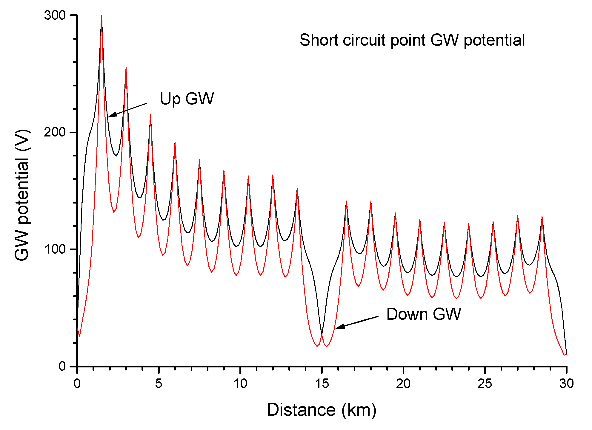
5.5. Effect of Directly Buried Ground Wire

The section considers the scenario where two directly buried ground wires (GWs) are laid along the track as shown in Figure 4. The value of the rail potential at the train position where there is a 1000 A load current scan from 0 to 30 km up the track is shown in Figure 9. The potential and the maximal current of the buried bare wire are shown in Figure 10 and Figure 11, respectively.

Table 1. Effect of the GW cross-section.

Wire Type	Maximal Rail Potential	Maximal GW Current
TJ25	89.7 V	74.8 A
TJ35	88.5 V	94.2 A
TJ50	87.3 V	118 A
TJ70	86.4 V	142 A
TJ95	85.9 V	162 A

shows the maximal rail potential and maximal buried ground wire current under the condition of ground wires with different cross-sections. It reveals that the main function of the directly buried ground wire is to decrease the shunt leakage resistance of the return circuit, meaning a relatively small cross-section will be enough.

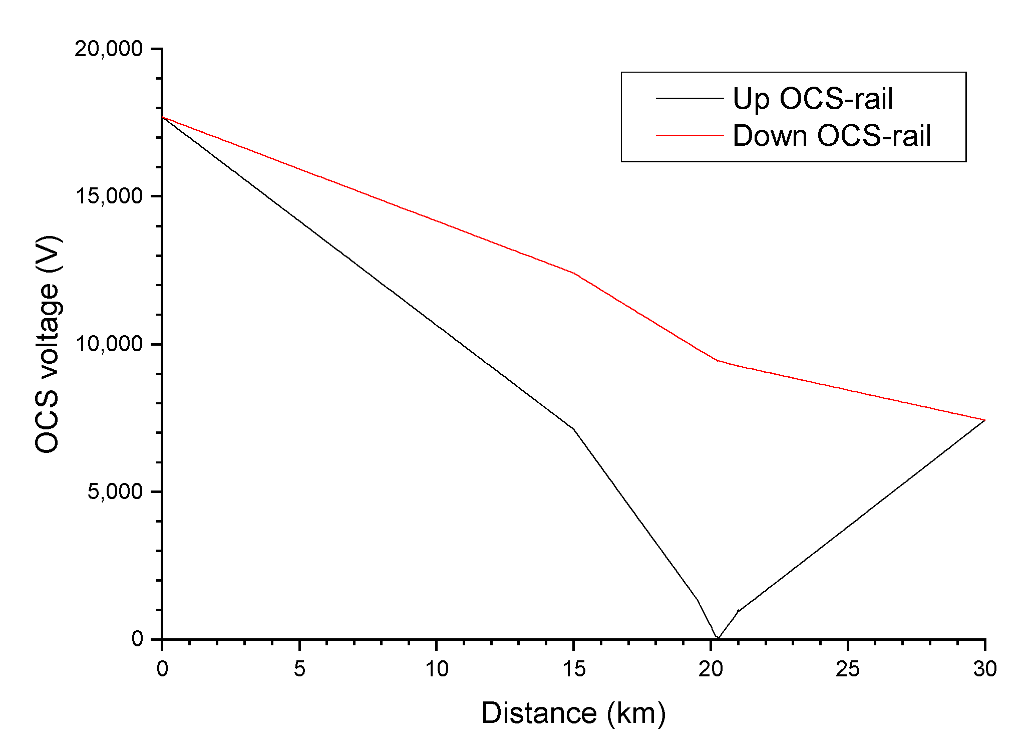
5.6. T–R Short Circuit

Suppose a T–R short circuit takes place up the track. The short-circuit current, rail potential and GW potential are shown in Figure 12, Figure 13 and Figure 14, respectively.

For the scenario where the short-circuit point is at 20.25 km, the relative potential and current profile are shown in Figure 15, Figure 16, Figure 17 and Figure 18 (5809 A for the short-circuit current).

5.7. T–PW Short Circuit

Suppose a T–PW short circuit takes place up the track. The PW potential at the short-circuit point is shown in Figure 19. For the scenario where a PW and GW are connected additionally at 500 m and 300 m intervals, the variation in the PW potential is shown in Figure 20.

6. Field Test

A field test was carried out on a T–R+NF traction network of a railway line in China (Figure 21), where a ground wire (70 mm² copper) was buried. Figure 22 shows the measured rail potential as well as the ground wire potential when the rail disconnected from or connected to the ground wire. It can be seen that when the rail disconnected from the ground wire, the maximum potential of the rail reached 18V. After the rail connected to the ground wire, the maximum dropped to 12 V, a one-third decrease. This decrease is obviously beneficial to improving safety. In fact, the implementation of the ground wire decreased the synthetic leakage resistance of the traction return network to the ground.

7. Conclusions

Due to the heavy loads, large short-circuit currents and high rail–ground leakage resistance, the rail potential of high-speed railways can be remarkably higher than that of conventional electric railway lines. Proper countermeasures must be taken to suppress the rail potential to an acceptable level.

In view of economy and reliability, to decrease the rail potential, firstly, we should try to decrease the longitudinal serial impedance of the traction return circuit, i.e., bond rails of different tracks, or adequately add CPWs. Secondly, the natural grounding resistances of various structures along the railway should be utilized if it is possible to decrease the transversal shunt conductance of the traction return circuit. Finally, directly buried ground wires and a dedicated grounding pole can be laid out or constructed to suppress the rail potential further. Adding GWs can decrease the rail potential remarkably. Furthermore, GWs provide a common grounding possibility along the railway line. The main function of GWs is to decrease the shunt leakage resistance of the return circuit, rather than to conduct return currents, meaning a relatively small cross-section will be enough.

It should be pointed out that, on the other hand, decreasing the rail potential will lead to an increase in the earth current. The earth current can also contribute to the interference of railway signal systems. A compromise must be made between suppressing the rail potential and increasing the immunity of signal equipment to EMI conducted and/or inducted by traction power supply systems.

The grounding of traction networks is a complex problem. Different countries may have different schemes. Now, the so-called integrated grounding technique seems to be the preference for newly built high-speed railways. The discussion of this paper is only from the point of view of power supply engineering.

References

1. Gu, J.; Yang, X.; Zheng, T.Q.; Shang, Z.; Zhao, Z.; Guo, W. Negative Resistance Converter Traction Power System for Reducing Rail Potential and Stray Current in the Urban Rail Transit. IEEE Trans. Transp. Electrif. 2021, 7, 225–239. [Google Scholar] [CrossRef]
2. Huang, K.; Liu, Z.; Zhu, F.; Deng, Y. Grounding Behavior and Optimization Analysis of Electric Multiple Units in High-Speed Railways. IEEE Trans. Transp. Electrif. 2021, 7, 240–255. [Google Scholar] [CrossRef]
3. Natarajan, R.; Imece, A.; Popoff, J.; Agarwal, K.; Meliopoulos, P.S. Analysis of grounding systems for electric traction. IEEE Trans. Power Deliv. 2001, 16, 389–393. [Google Scholar] [CrossRef]
4. Kiesling, F.; Puschman, R.; Schmieder, A. Contact Lines for Electric Railways, Planning Design Implementation; Siemens: Munich, Germany, 2001. [Google Scholar]
5. Biesenack, H.; George, G.; Hofmann, G.; Schmidder, A. Electric Railway Traction Power Supply Systems (Translated by Guangfeng Qi); China Railway Press: Beijing, China, 2019. [Google Scholar]
6. Gu, J.; Yang, X.; Zheng, T.Q.; Xia, X.; Zhao, Z.; Chen, M. Rail Potential and Stray Current Mitigation for Urban Rail Transit With Multiple Trains Under Multiple Conditions. IEEE Trans. Transp. Electrif. 2022, 8, 1684–1694. [Google Scholar] [CrossRef]
7. Wang, M.; Yang, X.; Zheng, T.Q.; Ni, M. DC Autotransformer-Based Traction Power Supply for Urban Transit Rail Potential and Stray Current Mitigation. IEEE Trans. Transp. Electrif. 2020, 6, 762–773. [Google Scholar] [CrossRef]
8. Wang, Y.; Zhang, G.; Qiu, R.; Liu, Z.; Yao, N. Distribution Correction Model of Urban Rail Return System Considering Rail Skin Effect. IEEE Trans. Transp. Electrif. 2021, 7, 883–891. [Google Scholar] [CrossRef]
9. Chen, M.; Fu, H.; Xie, C.; Liu, W.; Xu, W. Analysis of Rail Potential Characteristics of AC/DC Dual-system Traction Power Supply System. Xinan Jiaotong Daxue Xuebao J. Southwest Jiaotong Univ. 2022, 57, 729–736. [Google Scholar] [CrossRef]
10. Kaleybar, H.J.; Brenna, M.; Foiadelli, F.; Fazel, S.S.; Zaninelli, D. Power Quality Phenomena in Electric Railway Power Supply Systems: An Exhaustive Framework and Classification. Energies 2020, 13, 6662. [Google Scholar] [CrossRef]
11. Song, S. Study on the Feature of Running-through Earth Wire and Impact on Traction Currents Distribution in High-speed Railway; Beijing Jiaotong University: Beijing, China, 2017. (In Chinese) [Google Scholar]
12. Yang, B. Comprehensive Simulation of AT Traction Power Supply and Integrated Grounding System; Beijing Jiaotong University: Beijing, China, 2014. (In Chinese) [Google Scholar]
13. Wu, G.; Gao, G.; Dong, A.; Zhou, L.; Cao, X.; Wang, W.; Wang, B.; Tang, Y.; Chen, J. Study on the Performance of Integrated Grounding Line in High-Speed Railway. IEEE Trans. Power Deliv. 2011, 26, 1803–1810. [Google Scholar] [CrossRef]
14. Ning, B.; Tang, T.; Dong, H.; Wen, D.; Liu, D.; Gao, S.; Wang, J. An Introduction to Parallel Control and Management for High-Speed Railway Systems. IEEE Trans. Intell. Transp. Syst. 2011, 12, 1473–1483. [Google Scholar] [CrossRef]
15. Guemes, J.A.; Hernando, F.E. Method for calculating the ground resistance of grounding grids using FEM. IEEE Trans. Power Deliv. 2004, 19, 595–600. [Google Scholar] [CrossRef]
16. Guemes-Alonso, J.A.; Hernando-Fernandez, F.E.; Rodriguez-Bona, F.; Ruiz-Moll, J.M. A practical approach for determining the ground resistance of grounding grids. IEEE Trans. Power Deliv. 2006, 21, 1261–1266. [Google Scholar] [CrossRef]
17. Huang, W.; He, Z.; Hu, H.; Wang, Q. Study on Distribution Coefficient of Traction Return Current in High-Speed Railway. Energy Power Eng. 2013, 5, 1253–1258. [Google Scholar] [CrossRef]
18. Riordan, J. Current propagation in electric railway propulsion systems. AIEE Trans. 1932, 51, 1011–1019. [Google Scholar] [CrossRef]
19. Watanabe, H.; Mochinaga, Y. Rail potential and countermeasures for rail potential suppression of electric railways. Railw. Tech. Res. Rep. 1978. [Google Scholar]
20. Qi, G.; Xin, C. Voltage and Current Distribution of Rail Circuit and the Integrated Grounding System for High Speed Railway Traction Network; Southwest Jiaotong University Press: Chengdu, China, 2012. [Google Scholar]
21. Zhao, T.; Wu, M. Electric power characteristics of all-parallel AT traction power supply system. In Proceedings of the 2011 International Conference on Transportation, Mechanical, and Electrical Engineering (TMEE), Changchun, China, 16–18 December 2011. [Google Scholar] [CrossRef]
22. Zhang, J.; Wu, M.; Liu, Q. A Novel Power Flow Algorithm for Traction Power Supply Systems Based on the Thévenin Equivalent. Energies 2018, 11, 126. [Google Scholar] [CrossRef] [Green Version]
23. Mingli, W.; Yu, F. Numerical calculations of internal impedance of solid and tubular cylindrical conductors under large parameters. IEEE Proc. Gener. Transm. Distrib. 2004, 151, 67–72. [Google Scholar] [CrossRef]
24. Carson, J.R. Wave propagation in overhead wires with ground return. Bell Syst. Tech. J. 1926, 5, 539–554. [Google Scholar] [CrossRef]
25. PoIlaczek, F. Uber das Feld einer unendlich langen wechselstrom-durchflossenen Einfachleitung. Elekt. Nachr. Tech. 1926, 3, 339–359. (In German) [Google Scholar]
26. Dommel, H.W. EMTP Theory Book, 2nd ed.; Microtran Power System Analysis Corporation: Vancouver, BC, Canada, 1992. [Google Scholar]
27. CCITT. Directives Concerning the Protection of Telecommunication Lines against Harmful Effects from Electric Power and Electrified Railway Lines; International Telecommunication Union: Geneva, Switzerland, 1989; Volumes I and IV. [Google Scholar]
28. Sunde, E.D. Earth Conduction Effects in Transmission Systems; D. Van Nostrand Company, Inc.: New York, NY, USA, 1949. [Google Scholar]
Figure 1. Rail current and potential.
Applsci 13 07944 g001
Figure 2. Overhead conductors.
Applsci 13 07944 g002
Figure 3. Directly buried bare conductors.
Applsci 13 07944 g003
Figure 6. Effect of bonding.
Applsci 13 07944 g006
Figure 7. Effect of rail leakage resistance.
Applsci 13 07944 g007
Figure 8. Effect of OCS post resistance.
Applsci 13 07944 g008
Figure 9. Rail potential with the directly buried bare wire.
Applsci 13 07944 g009
Figure 10. Potential of the directly buried bare wire.
Applsci 13 07944 g010
Figure 11. Maximal current of the directly buried bare wire.
Applsci 13 07944 g011
Figure 12. Short-circuit current at different positions.
Applsci 13 07944 g012
Figure 13. Rail potential at the short-circuit point.
Applsci 13 07944 g013
Figure 14. Potential of the directly buried bare wire at the short-circuit point.
Applsci 13 07944 g014
Figure 15. OCS–rail voltage.
Applsci 13 07944 g015
Figure 16. Rail potential.
Applsci 13 07944 g016
Figure 17. GW current.
Applsci 13 07944 g017
Figure 18. GW potential.
Applsci 13 07944 g018
Figure 19. PW potential at the short-circuit point.
Applsci 13 07944 g019
Figure 20. Effect of the connection of the PW and GW.
Applsci 13 07944 g020
Figure 21. Photo of the field test.
Applsci 13 07944 g021
Figure 22. Measured data of rail and ground wire potentials: (a) when the rail disconnected from the ground wire; (b) when the rail connected to the ground wire.
Applsci 13 07944 g022