Abstract
Characterizing the electric energy curve can improve the energy efficiency of existing buildings without any structural change and is the basis for controlling and optimizing building performance. Artificial Intelligence (AI) techniques show much potential due to their accuracy and malleability in the field of pattern recognition, and using these models it is possible to adjust the building services in real time. Thus, the objective of this paper is to determine the AI technique that best forecasts electrical loads. The suggested techniques are random forest (RF), support vector regression (SVR), extreme gradient boosting (XGBoost), multilayer perceptron (MLP), long short-term memory (LSTM), and temporal convolutional network (Conv-1D). The conducted research applies a methodology that considers the bias and variance of the models, enhancing the robustness of the most suitable AI techniques for modeling and forecasting the electricity consumption in buildings. These techniques are evaluated in a single-family dwelling located in the United States. The performance comparison is obtained by analyzing their bias and variance by using a 10-fold cross-validation technique. By means of the evaluation of the models in different sets, i.e., validation and test sets, their capacity to reproduce the results and the ability to properly forecast on future occasions is also evaluated. The results show that the model with less dispersion, both in the validation set and test set, is LSTM. It presents errors of −0.02% of nMBE and 2.76% of nRMSE in the validation set and −0.54% of nMBE and 4.74% of nRMSE in the test set.
1. Introduction
Complying with measures to reduce global warming leads to electrification. This transition has a large impact on the building sector, where an increase in electric energy is expected [1,2]. The increase in demand is mainly generated by the conversion of thermal to electrical consumption through HVAC systems, and there is a worldwide trend for interconnection of essential appliances by means of the Internet, forming the IoT [3,4]. Electrical vehicles also have a significant influence on the increase in demand due to their need for charging points in buildings [5,6].
The design of existing buildings was carried out in the past without sufficient consideration for climatic conditions as it was possible to improve the building performance without any structural change through the optimization of its loads [7,8]. This, together with the fact that today the building sector causes of emissions in Europe, means that improving energy efficiency in existing buildings is extremely important [9]. It is estimated that an improvement in building performance could reduce emissions by more than , which makes it possible to be in line with the measures adopted for global warming [10].
The great impact on the building sector of greenhouse gases makes it necessary to reinforce studies on techniques that allow efficient management of energy use [11]. Current research leads to emission reductions by combining distributed generation and storage [12,13]. This combination allows buildings with reduced use of electrical network needs to become zero-emission buildings (ZEB) [14,15]. The resilience and effectiveness in the implementation of these techniques depends on the recognition of the variations that occur in the electric energy [16]. By obtaining predictive models, the contribution needs are estimated, thus increasing the impact on the reliability of the operations.
There has been much data collection on existing buildings in recent years due to the installation of smart meters and the development of IoT technology. Artificial intelligence (AI) techniques take advantage of this large amount of data to accurately forecast a variable [17,18]. In addition, AI models are characterized by their strong ability to adjust and learn in real time, which increases the reliability of decision making in energy management and which is important considering the transition to ZEB [19,20]. Since it is desired to model a target forecast based on some independent variables, the branch of AI used to carry out this research must be pattern recognition. This method can characterize complex non-linear problems accurately with reduced computation times [21,22].
This paper intends to evaluate the performance in electric energy forecasting of some of the typical methods used in the resolution of complex patterns in the field of energy. On the one hand, random forest (RF), support vector regression (SVR), and extreme gradient boosting (XGBoost) are implemented as more classical machine learning (ML) techniques. On the other hand, multilayer perceptron (MLP), which is representative of feedforward artificial neural networks (ANN), long short-term memory (LSTM), a type of recurrent neural network (RNN), and a temporal convolutional network (Conv-1D), a representative model of convolutional neural networks (CNN), are employed to characterize the deep learning (DL) techniques.
The transition to electrification requires significant changes in the building sector to improve its performance. The AI techniques offer many possibilities due to their accuracy and short computation times. In addition, the aforementioned models are flexible, adjusting in real time to the needs that are constantly presented in ZEBs. In recent years, multiple studies have been carried out applying these models to problems in the field of energy. However, it remains unclear which is the most reliable model in determining the forecast of electrical loads in the building sector. Thus, the aim of this paper is to analyze the most typical ML and DL techniques employed for regression, determining their quality and possible use in forecasting electric energy by analyzing their bias, variance, and performance to forecast future timesteps. The models are evaluated in an existing building allowing the presence of missing values and using k-fold cross-validation to guarantee the reproducibility of the results obtained. In addition, a seed is used to effectively compare the models.
Thus, the main contribution of this paper is to compare different ML and DL techniques to determine which are most suitable for forecasting electricity consumption in buildings. The methodology conducted considers:
- The dispersion of the different AI models with respect to the real data and how each model varies in the different folds to effectively determine the variance of the results with respect to the real data.
- The tendency of the AI models to overpredict or underpredict the data in the different folds to determine the bias of these with respect to the real data.
- The projection to the future by application to a dataset used to reproduce the behavior of the AI models in a composition different from the one used in the training.
The content of this paper is organized as follows: background about the AI models used is presented in Section 2; the utilized methodology to compare the different AI techniques is explained in Section 3; the studied building, and the specific characteristics of the DL and ML tried are presented in Section 4; the evaluation of the model forecasts of electricity consumption is reported in Section 5; the reliability of the developed techniques is discussed in Section 6; and the conclusions are outlined in Section 7.
2. Related Work
Electricity consumption forecasting plays a vital role in efficient energy management and planning in buildings. Research in this field focuses on investigating topics such as smart grids, renewable energy integration or local energy communities [23,24]. ML and DL models have revolutionized this research by providing accurate and reliable predictions.
Time series models like the autoregressive integrated moving average model (ARIMA) or the seasonal autoregressive integrated moving average (SARIMA) have long been used for energy forecasting in this sector, capturing seasonality and trends in historical consumption data [25,26]. However, with advancements in ML and DL models like those presented in this study, powerful tools for capturing complex patterns and dependencies in electricity consumption have emerged. These models can handle non-linear relationships and long-term dependencies, making them suitable for energy forecasting in buildings [22]. Hybrid models that combine multiple forecasting techniques have also shown promise, leveraging the strengths of different algorithms to enhance prediction accuracy [27,28].
The effectiveness of ML and DL models relies on feature engineering techniques that extract relevant information from the data, enabling the models to capture the key factors influencing electricity consumption. The application of these techniques enables better energy management decisions, facilitates grid stability, and supports the integration of distributed generation [29,30]. The continuous advancements in this field provide precise and timely forecasts for effective energy planning and optimization.
In [31], a method is presented that generates parallel energy consumption data using generative adversarial networks (GAN) and combines the generated data with the original data to improve the performance of energy consumption prediction in buildings. The authors use MLP, XGBoost and SVR, and evaluate the results using mean absolute error (MAE), mean absolute percentage error (MAPE) and Pearson correlation coefficient®. In [27], a method is proposed that jointly integrates the CNN and LSTM for the prediction of electric charges. The authors compare performance with other models, i.e., LSTM, XGBoost, and radial basis functional network (RBFN), by using root mean square error (RMSE), MAPE metrics. MAE and goodness of fit (R2).
In [32], a non-parametric regression model is proposed to predict electricity consumption in buildings. The model uses the Gaussian process (GP) for the selection of the input data. In the study, SVR, LSTM and RF are evaluated to compare the effectiveness of the proposed model. The error evaluation is carried out with symmetric mean absolute percentage error (sMAPE), MAE and RMSE. The study carried out in [28] develops strategies for predictive control using neural networks to predict energy consumption in buildings. The MLP and its optimization with the Levenberg–Marquardt algorithm are evaluated. The performance is evaluated with MAE and RMSE.
In [33], an analysis is carried out that evaluates the performance of RF, regression tree (RT) and SVR for the prediction of energy consumption in buildings. The evaluation indices are MAPE, R2, RMSE and PI. In [34], the authors compare the gradient boosting (GB), RF, and time of week and temperature model (TOWT) methods for predicting energy consumption in buildings by applying cross-validation. In this analysis, the performance of the models is evaluated using R2, coefficient of variation of the RMSE (CV(RMSE)) and normalized mean bias error (nMBE).
In [25], various techniques for predicting building loads are compared. LR, LSTM and ARIMA are used. The evaluation of the error is performed using RMSE and mean bias error (MBE). This same comparative analysis is carried out in [26], where the authors compare MLP, SVR, RT, linear regression (LR) and SARIMA. The performance of the models is determined with R, RMSE, MAE, MAPE and maximum absolute error (MaxAE). This same approach is carried out in [35], where the authors compare ARIMA, SARIMA, XGBoost, RF and LSTM by mean percentage error (MPE), MAPE, MAE and RMSE metrics. The authors of [36] investigate the use of SVR as a method for load prediction through a comparison with RF, ARIMA, XGBoost, and MLP, and the accuracy is assessed using MAPE.
In [37], the prediction of electricity consumption each day of the week is evaluated by means of a CNN, comparing the results with RNN, ARIMA and MLP. MAPE, MAE and RMSE are used for error evaluation. The approach of [38] proposes to predict electricity demand by separating building baseload power from occupant-influenced demand. A three-hour redundancy period is added to account for flexible working hours. The method used is MLP and its performance is evaluated with RMSE. In [39], the methods for the prediction of electricity consumption in a building are evaluated. The authors use different metrics to assess performance, i.e., RMSE, MAE, magnitude of relative error (MRE), MAPE, and normalized mean bias error (nRMSE).
In [40], a comparative analysis of the prediction of the energy demand of a building is carried out considering LR, SVR, MLP, extreme deep learning (EDL) and GBoost. To determine the most appropriate model, the performance is evaluated through cross-validation using the metrics R, MAE, RMSE, relative absolute error (RAE) and root relative squared error (RRSE). The framework adopted in [41] evaluates XGBoost, SVR and MLP for the prediction of the energy consumption of a building. Using a cross-validation model, the authors perform a performance assessment with CV(RMSE) and nMBE. Table 1 shows the main characteristics of each of the investigations discussed.

Table 1.
Summary of the main characteristics of the current research in the field of energy forecasting in buildings.
This study proposes a robust methodology for the prediction of electricity consumption considering the trends of different ML and DL models. Furthermore, we carry out a test to show the performance of the results obtained, showing the models’ effectiveness for prediction of moments in the test, including the validation, and future moments, i.e., the test set. This work aims to address the gaps in current studies, which are outlined below:
- Despite the great opportunity presented by ML and DL algorithms, the characteristic variability of the different techniques has not been evaluated. Many studies focus on LSTM, MLP, RF or XGBoost but do not compare the quality of the results with those of classic ML and DL methods.
- The evaluation of the models is carried out with a multitude of techniques, without considering the independence or significance of each of the metrics used. Therefore, studies report results a priori that are precise but without any meaning beyond the value obtained.
- Many studies lack techniques that show the robustness of the models evaluated. Thus, the use of cross-validation is not common. In this way, the results shown present a great dependence on the data sample used. Therefore, the reproducibility and use of the techniques with future datasets is limited.
3. Methodology
This section describes the techniques used for prediction of electrical loads in buildings. First, the techniques used to arrange the data into effective models are described in Section 3.1. Then, the ML and DL methods developed in this study are presented in Section 3.2. Finally, the performance indicators used to evaluate the forecast quality of the developed models are mentioned in Section 3.3.
3.1. Preprocessing
AI techniques are highly dependent on the quality and format of the dataset. The development of preprocessing processes in which the variables are chosen, and the data are filtered and transformed into an understandable format by the models is very important [42]. The data collection process may be affected by errors in communication or data collection, which frequently results in missing values in the final stage. Furthermore, monitoring programs collect a wide variety of parameters, not all of which are useful for the prediction of the target variable.
To recognize the most suitable dataset, a feature engineering stage is performed where, through plotting, the curves of the different variables that affect the target feature are visually characterized. This stage also allows the extraction of information that is not available as a variable in the dataset, but infers the variability of the objective feature, i.e., hour of the day, day of the week, or day of the year.
The selected data include the building parameters, weather conditions and temporal parameters. The building parameters are presence of occupants and electrical loads, and the weather conditions include the outdoor temperature. The temporal parameters are the hour of the day, day of the week and day of the year. Thus, from the input variables presence, temperature, hour of the day, day of the week, and day of the year, it is intended to forecast the output variable electrical loads.
The input variables were selected due to their inherent relationship with the variations in the output variable. Therefore, the presence of occupants allows the models to extract the behavior of the building occupants, outdoor temperature is related to the consumption of most of the devices, and temporal variables allow the recognition of demand curves through the different periods. Furthermore, hour of the day allows the extraction of daily patterns, while day of the week provides weekly patterns, and day of the year allows the recognition of seasonal patterns.
Pattern recognition from the models used is improved with the use of a data cleansing stage. In this stage, the data are filtered to detect outliers [43,44]. Because of the high instantaneous variability in electricity consumption, the methodology used is based on the interquartile range. The process is conducted iteratively to reduce the errors caused in the trends by these anomalous values. Thus, values outside the ranges given by (1) and (2) are not considered valid.
where and are the upper bound and lower bound, respectively, and are the third and the first quartile, and is the interquartile range.
The values recognized as outliers as well as the non-existent values in the dataset are kept as missing. In cases where there is a period of three timesteps or less, the gap is interpolated. This allows more data to be fed to the model without inferring too much error. The values established as missing are masked so that the AI algorithms interpret and work with them. The AI methodologies developed are more accurate when the variables they include have a similar data range, so a scaling stage is needed. On the one hand, the building parameters and weather conditions are standardized by subtracting the standard deviation and dividing it by the mean. On the other hand, a feature engineering process is performed on the temporal parameters by applying sine and cosine functions.
This scaling method was applied because it was verified in this study that dividing the building parameters and weather conditions by the mean offers more adjusted values in the residual demands. The application of sine and cosine functions has two reasons. Firstly, it increases the number of input features so that more parameters are related to the output variable and the models have more capacity of to extract the patterns. Secondly, it reduces the increasing influence of these variables. Thus, adding the variability of sine and cosine functions results in better forecasting [45].
3.2. Modeling
Training was conducted through a cross-validation procedure to ensure the quality of the models applied. This technique is used to guarantee that in each of the splits, the results are independent of the training, thereby minimizing overfitting in the modeling [46]. Thus, the training process is performed in one subdivision, corresponding to 80% of the training data, and the efficiency of the model is evaluated in another, which includes the rest of the training data. This process is carried out repetitively, exchanging the position of the validation throughout the training set.
In addition, the training process is conducted with mini-batch gradient descent, which avoids standstill at a local minimum and increases the level of convergence of the model [47]. Once the training process with these techniques has been carried out, the model is evaluated on the test sample.
This section explores the capabilities and reports the suitability of the different ML and DL models evaluated in this manuscript for the electricity load forecasting. Thus, the basics of the ML models are presented, starting with RF, and followed by SVR and XGBoost. Next, the characteristics of the DL models are introduced, starting with MLP and followed by LSTM and Conv-1D.
3.2.1. Random Forest
Random forest is a method that consists of the simultaneous operation of multiple uncorrelated decision trees. The training process, based on bootstrapping, is carried out by generating random subsamples from the training set. Through these subsamples, different models are generated and trained independently through random features selection. Once the models have been trained, the aggregating proceeds, generating assembled results through the average of the forecasted values of each of the decision tree models made. The combination of these techniques is also known as bagging. Bootstrapping ensures that the same data are not used for all trees, and random features selection reduces the correlation between trees [48,49,50]. Thus, by means of the training carried out with bagging, the RF enables improvements in the generalization by reducing the sensitivity of the model to the variations in the data [51]. The difficulty that the presence of different decision trees adds to the RF defines it as a black box technique since, as discussed in (3), the forecasted variable depends directly on the scores of each of the trees.
where is the forecasted variable, is the number of trees, and is the probability function of the forecasted variable given the independent variables.
Thus, because of the dependence of the decision trees, the objective function , in addition to seeking to minimize the error, considers the complexity of the set of decision trees, as shown in (4).
where is the number of samples, is the forecasted variable at time , and the difficulty of each of the decision tree is given by the function .
RF is a commonly used ML algorithm that can be advantageous for electricity consumption forecasting. The principal advantages of this model are as follows:
- Robustness: It can handle electricity fluctuations due to its robustness against noise and outliers in data.
- Non-linearity: It is capable of capturing non-linear relationships effectively, allowing it to model the complex dependencies presented in the electricity consumption.
- Scalability: It can handle large datasets efficiently and scale well with increasing data information.
- Out-of-the-box performance: It provides good performance with low hyperparameter tuning.
3.2.2. Support Vector Regression
The learning of the support vector regression is carried out to approximate the input data to a regression line considering a threshold. In this model, the trend line that best fits the data is called the hyperplane, and the lines delimiting the threshold are the boundary lines [40,52]. Thus, in SVR, the model maps the training data using a series of mathematical equations, known as kernels, to obtain the hyperplane containing the largest amount of input data within the boundary lines. The radial basis function (RBF) is a very frequent kernel similar to the Gaussian distribution [53,54] (5).
where is the variance, is the point being evaluated, is the orthogonal representation of in the hyperplane, and represents the kernel between the set of points to be evaluated, i.e., and its orthogonal representation .
The main difference between this model and typical linear regression is that the objective function seeks to fit the data within a range, rather than minimizing the error between forecasted and real data (empirical risk minimization). This feature allows SVR to represent linear and non-linear functions [36,43]. Thus, denoting the slack margin of the model as , the objective function can be defined as in (6):
where is the number of independent variables, and is a hyperparameter that represents the regularization. Therefore, if increases, the tolerance of out-of-bound values also increases. On the other hand, if approaches 0, the tolerance does too, which simplifies the problem and, therefore, does not consider the effect of slack [55].
SVR is a powerful ML algorithm that can be beneficial for electricity load forecasting due to several reasons. The main ones are presented below:
- Non-linearity: It can effectively capture non-linear relationships between electricity consumption and important features.
- Robustness to outliers: Due to its structure, it is less sensitive to outliers.
- Tunability: It has parameters that can be adjusted to control the balance between model complexity and generalization to adapt better to the fluctuations in electricity data.
- High-dimensional data: It can handle a large number of features without sacrificing performance.
3.2.3. Extreme Gradient Boosting
Extreme gradient boosting follows the principles presented in random forest. The main idea is improving the convergence of the RF by improving the adjustment of weak learners, or trees, whose forecasts do not have large adjustments [34,56,57]. To carry out this process efficiently, XGBoost uses additive training in which the previous iteration is considered as the actual forecast [58,59] (7).
where the superscript indicates the iteration considered.
This application of the addition technique also generates a slight modification in the calculation of the cost function , which considers both current and previous iterations (8). The benefit of using this technique is that the loss function expands to the second order, making it possible to optimize the problem quickly [41].
XGBoost is a popular ML technique that can handle electricity consumption forecasting. The main reasons are presented in following points:
- Regularization and control: It offers various regularization techniques to control the complexity of the data, which prevent overfitting and improve generalization.
- Non-linearity: It captures non-linear relationships in electricity consumption to model its complex relationships.
- Scalability and efficiency: It is suitable for handling large datasets with high-dimensional feature spaces.
- Flexibility: It has a wide range of hyperparameters that can be tuned to optimize the model’s performance.
3.2.4. Multilayer Perceptron
Feedforward artificial neural networks, mostly implemented using MLP, are composed of three types of interconnected layers: an input layer, where the input features are located; an output layer, where the forecasted variable is established; and some hidden layers, which correspond to the internal layers of the model. The connections between them are based on a weight structure, and the hidden layers are responsible for extracting patterns from the data and storing them during the training phase Each of the layers has its own neurons [60,61]. The number of input neurons is normally equal to the number of features; the number of output neurons is the same as the number of variables to be predicted; and the number of hidden neurons, as well as the number of hidden layers, depend on the problem. As the hidden layers or hidden neurons increase, the ability of the model to extract hard patterns increases; however, the problem becomes more complex [62,63]. This rule is not always fulfilled since as the number of hidden layers or hidden neurons increases, the model has a greater tendency to suffer from overfitting [64]. Therefore, the forecasted variable depends on the variety of the hidden layers and hidden neurons. Therefore, similar to RF and the XGBoost, this is a black box model. In this case, the internal operations of the neurons depend on the activations of the preceding neurons. In (9), the process that governs the behavior of neurons can be seen in detail.
where corresponds to the function of the studied neuron, is the activation function of preceding neuron, and and are the weights of the neuron connection and bias, respectively.
This process is propagated from the input layer to the output layer through the interconnections of the neurons. Furthermore, if a node has more than one input, the final value of the function of this node corresponds to the sum of the individual values of the functions of the node and their connections. The end of each step performed in the iterative training process is terminated by backward propagation, where the error is propagated to the input layers, and updating the values of the weights [65,66]. As in MLs, learning is based on minimizing a cost function . In this case, the cost function is governed by (10).
where is the objective variable at time , and is the predicted series of the objective variable at time .
MLP is a commonly used DL model. Its structure is beneficial for electricity consumption forecasting. The following are some important advantages of this technique:
- Non-linear: It is capable of modeling non-linear relationships.
- Flexibility and adaptability: It has a high number of hyperparameters that offers this model flexibility in terms of network architecture and activation functions.
- Missing data: It can handle missing data effectively.
- Adaptability to changing patterns: It has the ability to learn and adapt to changes in complex patterns in data.
3.2.5. Long Short-Term Memory
Recurrent neural networks are a derivative of ANNs, so the learning process is carried out in a similar way to that presented in the previous section. Thus, the minimization process is governed, as in the previous case, by Equation (8). The RNN and the ANN are usually used together, where the first layers of the problem are part of the RNN. These layers extract and retain all possible information from the data, and the subsequent layers form the ANN. Because of the internal complexity of the RNNs arising from the need to train a larger number of parameters, they tend to cause problems of overfitting [67,68].
The main characteristic of RNNs is the retention of important information from the dataset [69]. The best known and commonly used model is LSTM. This model consists of a series of internal mechanisms to regulate the flow of relevant information in the short and long term to make accurate forecasts. This flow of information is transferred in sequence by the cell state, where the retention of relevant information and the elimination of irrelevant information is controlled by gates [70,71,72]. In each neuron, the flow of the LSTM is controlled by 3 types of gates: forget gates, input gates, and output gates. If a node has more than one input, its function corresponds to the sum of the resulting values of each of its connections. This process propagates from the input neurons to the output neurons through the interconnections [70].
The forget gate, given in (11) by , decides which information that has been previously retained should be kept or deleted when new data are received.
where is the kernel, a function of the information previously kept, , and the new data, , and is the bias of the forget gate. is the activation function. The sigmoid activation function is commonly used because it compresses the information in the range [0, 1]. This allows the gate to recognize when the information is important, i.e., whether the value is close to or equal to 1, or when it is irrelevant, i.e., whether the value is close to or equal to 0.
The input gate decides what new information should be stored in the cell state through the simultaneous operation of 2 steps. Firstly, (12) determines what information should be updated, . Then, through (13), the sequence, , is regulated.
where and are the weights of the phase of information retention of the input gate, kernel, and bias, respectively. As in the forget gate, the sigmoid activation function is frequently employed to retain important information.
where and are the weights of the phase of sequence regulation of the input gate, kernel, and bias, respectively. In this case, the tanh activation function is commonly utilized because it compresses the information in the range [−1, 1]. This adds a weight to the values obtained in the previous phase in the cell state.
By combining the results of the previously described gates and the previous information kept in the cell state, , the value of the cell state, in Equation (14), is updated.
Finally, the output gate decides the output of the neuron. This is the combination of the information previously kept together with the new data and information resulting from the cell state (15).
where and are the weights of the information previously retained together with the new data, kernel, and bias, respectively. is the activation function corresponding to this set of information. Sigmoid activation function is commonly used to select which of the previous values are retained. is the activation function of the cell state. The tanh activation function is employed to give weights to these retained values.
LSTM can be advantageous for electricity loads forecasting. The main reasons are as follows:
- Temporal modeling: It is specifically designed to model temporal dependencies in data.
- Context preservation: It can capture short-term dependencies and accommodate irregular or missing data points due to its long-term memory.
- Scalability: It can effectively capture complex patterns from extensive historical data.
- Robustness: It is robust against noise and outliers in data.
3.2.6. Temporal Convolutional Networks
The convolutional neural networks are also a derivative of ANNs, so the learning process is carried out in a similar way to that presented above, seeking the minimization of (10). CNNs and ANNs are also often utilized together, where the first layers of the problem correspond to the CNN. Theses layers filter data and find relevant information from the data, and the subsequent layers comprise the ANN. This is due to the CNN reducing the dimensions of the data, keeping important details and avoiding irrelevant ones. Therefore, if CNN layers are used too many times in the problem, important patterns are lost, thus resulting in forecast failure [73]. This characteristic allows the CNN to simplify the problem, making in contrast to the RNN, the training more efficient [74]. The training process is carried out by Conv-1D and flattening layers.
Convolutional layers are the main structures of the Conv-1D. The process that this layer follows starts from an input vector, i.e., the input features, which is convoluted with kernels, i.e., the feature detector, to give as a result an output vector, i.e., the feature map. Thus, the feature detector moves over the input vector generating the dot product with the subregion of input vectors and obtains the feature maps as a matrix of the dot product. The feature detectors represent the weights of the previous deep learning methods presented. Instead of having individual weighs for each neuron, Conv-1D uses the same weights for all neurons. More feature detectors may result in better capture of input patterns. Nevertheless, this may cause some of them to take the same pattern, thus reducing the reliability of the method [75,76,77].
The shape of the feature map depends on the application of the convolution between the input vector and the feature detector. Stride and the padding also have an impact in the process (16). Stride refers to the number of moves from the feature detector to the input vector, and padding corresponds to the addition of an outer edge of zeros to the input vector [78,79].
where is the feature map, is the input vector, is the feature detector, is the padding, and is the stride.
Similar to the convolutional layers, flattening of layers reduces the dimensions of the convolved feature. This method is normally employed at the end of the convolution process. It transforms the feature map matrix into a single column that is fed to the ANN for processing [80,81].
Conv-1D offer several advantages for electricity demand forecasting. Some of them are as follows:
- Scalability: It can handle variable-length input sequences, accommodating missing data.
- Robustness: It is robust against noise and outliers in the data since it can detect and filter the irrelevant patterns.
- Global context: It captures global information and dependencies across different time scales.
- Interpretability: It allows better understanding of the patterns that contribute to electricity consumption.
3.3. Performance Evaluations
The models are evaluated by their ability to correctly predict the target variable. To adequately analyze the forecast obtained by the different models and avoid the randomness of the optimization process, a seed is used. Furthermore, to ensure the reproducibility of the obtained configurations, the cross-validation method is implemented. Thus, the performance analysis is realized in validation and test sets. To highlight different aspects that the models may present, they are evaluated by a group of metrics without interrelation. The dispersion, tendency, and capability to reproduce the results in actual and future time points are evaluated. These metrics are the normalized mean bias error (), and the normalized root mean squared Error (). The provides a measure of the general bias of a given variable, where positive and negative values represent underestimation or overestimation of the information, respectively (17).
where, is the maximum value of the objective variable.
The measures the variability in the errors between the measured and simulated values, thereby giving an indication of the model’s variance, as shown in (18). Thus, with the application of this formula, the normalized standard deviation of the predicted dataset is reflected with respect to the actual observation of these data.
4. Case Study
With the application of the methodology presented in the previous section, we determine the AI methods most suitable for modeling the behavior of electrical demand of a building. This is validated with a single-family dwelling located in the city of Maryland, United States [82,83]. The house has two floors divided into a kitchen, a living room, a dining room, four bedrooms, and three bathrooms. In the measurement period, the residence was operated in an all-electric configuration, with a simulated family of four people (two adults, and two children), who carried out typical American activities.
The measurements correspond to hourly data divided into two periods, the first, from 1 July 2013 to 30 June 2014, and the second from 1 February 2015 to 31 January 2016. The data selected for the purpose of validating the methodology presented in this study are presence, outdoor temperature, and electrical loads, where presence reflects the behavior of the inhabitants, and electric power demand corresponds to lighting and loads, both electrical and thermal. The data are of high quality, and there is a reduced number of wrong values in the whole dataset as a result of the preprocessing step: 0.99% in the case of presence, 1.95% in the case of outdoor temperature, and 1.18% in the case of electrical loads. The temporal parameters, i.e., hour of the day, day of the week, and day of the year, are extracted from the information provided by the data, so these features do not have incorrect values. By means of one-hot encoding, the models are capable of modeling with missing values to maintain the continuity in the dataset.
The data are standardized to obtain a precise adjustment in all the models used. The features presence, outdoor temperature, and electrical loads are normalized using their mean, and for the temporal parameters, sine and cosine functions are applied. The performance comparison of the models is obtained from the normalization of the metrics with the maximum value of electricity consumption in the series. Thus, from the , the variance of the models is estimated, and from the , the bias of the models is visualized. The capacity of the models to reproduce the results in different datasets is also evaluated through the evaluation of the results in different sets using a 10-fold cross-validation technique.
The methodology is applied using the k-fold method with ten folds. To compare the obtained results with the different methods, a seed is applied. The dataset is divided with 90% for the training set, 5% for the validation set, and the remaining 5% for testing. The models train through cross-validation in the training set, and accuracy is checked using the validation set. The test set is an independent set in which the final evaluation of the adjustments made by the models is realized. The training process is carried out using a patience of 100 epochs, a batch size of 64, and an Adam optimizer with a learning rate of 0.001.
The SVR model is constructed using a tolerance of 0.001 and a regularization parameter of 1. The MLP model is composed of four hidden layers with 100, 75, 50, and 25 neurons, respectively. The activation functions are linear for the first three hidden layers, and ReLU for the fourth hidden layer and the output layer. In the LSTM modeling, short-term memory is imposed on six timesteps, i.e., the 6 h prior to the instant to be forecast. The first hidden layer corresponds to the LSTM layer with 64 neurons. Then there are two more hidden layers with 40 and 20 neurons, which are dense layers. Linear and ReLU activation functions are used in these two hidden layers. The LSTM layer has predefined activation functions on its gates, and the output layer also has an ReLU activation function. The Conv-1D model starts with a convolutional layer with 64 filters and 3 feature detectors. In the convolution, padding is not added, and the stride is set to 1. Then, a flattening layer is applied for the imposition of two more hidden layers, defined as dense layers, with 40 and 20 neurons. The activation functions are linear for the convolutional layer and the hidden layer of 40 neurons, and ReLU is used in the rest of layers, i.e., the last hidden layer and the output layer. The hyperparameters used are summarized in Table 2.
Table 2.
Hyperparameter selection.
5. Results
This section discusses the adjustment of the different AI techniques carried out to forecast the electrical loads in an existing building, introduced in the first sentences of Section 4. The precision of these techniques has been obtained by means of the methodology described in Section 3 and the specific modeling characteristics presented in the final paragraphs of Section 4. In this section, the bias and dispersion of the accuracy in the models are evaluated for the validation and test sets. The analysis is carried out using 10-fold cross-validation. To compare the results between different models effectively, a seed is employed.
The distributions presented in the figures in this section are intended to show in detail the error distribution in the different folds. The adjustment of the different models is determined by evaluating their bias and variance. The box represents the interquartile range (IQR), the line that divides it is the median, the whiskers indicate the diversity within the accepted range, this being over and under the third and first quartiles, Q3 and Q1, respectively, i.e., or , and the circles correspond to outliers.
Figure 1 shows the bias of the models and the dispersion obtained by evaluating the errors using the metric in the validation set. The worst model is the SVR. This model presents an IQR of , a value higher by % with respect to the IQR of XGBoost, the model with the next highest rate. In addition, the median of the SVR is , this being in the model with the next highest error, XGBoost. Both XGBoost and RF present values above the ranges established as acceptable, i.e., . Thus, these show a higher IQR and, on certain occasions, anomalous values. This does not occur in the DL models, which are more stable in the training evaluation. The DL techniques also present a lower median, especially the values of LSTM and the MLP. The bias of these two models, in contrast to the other models which underpredict, have a slight tendency to overestimate, with values of in the case of LSTM and in the case of MLP. LSTM stands out, which also has a very tight IQR, with a value of .
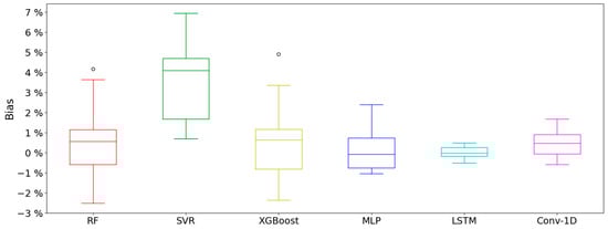
Figure 1.
Bias in the validation set of the different models using k-fold method.
Evaluating the fit of the metric in the test set, as presented in Figure 2, it can be seen that the SVR is still the model with the worst adjustment. In this case, its median is . Furthermore, two outliers are observed. However, it is the model with the lowest dispersion, with an IQR of . The rest of the ML also present a reduced dispersion, with an IQR of in the case of RF and in the case of XGBoost. Despite this, both models continue to have anomalous values, with 1 for RF and 3 for XGBoost. In contrast to what occurs in the training, the IQR of the DL in the test set is higher than the ML. The model with the greatest dispersion is the Conv-1D, with an IQR of . The median of this model is twice the value presented in the validation, growing from to . In this case, there is greater variation in the adjustment. The rest of the models have a variation from the median of about %. This affects the bias in the XGBoost and RF predictions, which change from underestimating to overestimating, and MLP, which changes to underestimating. The bias in the rest of the models remains stable, repeating the trend that occurs in the training. The most stable model is LSTM, which despite presenting a slightly worse fit, reduces the median by % and maintains the bias, i.e., continues to overestimate. It has an IQR similar to that of the training, which is % higher in the testing.
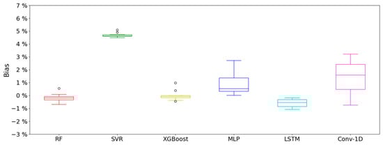
Figure 2.
Bias in the test set of the different models using k-fold method.
Figure 3 shows the variance in the predictions in the validation set from the calculation of the . The models with less divergence in the results are SVR and MLP, with IQR values of and , respectively. Nevertheless, these are the models that present the worst adjustments, with the median being and , respectively. In addition, both models present values above and below the ranges established as acceptable. Although RF and XGBoost improve the variance of the previously presented models and the medians are and , respectively, they also present anomalous values. In contrast, neither the Conv-1D nor the LSTM present anomalous values. The IQR of both models is similar: for Conv-1D, and for LSTM. The variance, based on its median value, is and , respectively. Thus, LSTM is shown to be the model with lower variance.
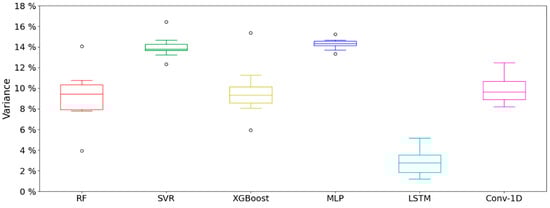
Figure 3.
Variance in the validation set of the different models using k-fold method.
The variance in the forecasts in the test set are shown in Figure 4. The variances of the SVR, MLP, and Conv-1D are the highest, with their medians being , , and , respectively. However, these are models with less dispersion in the results, with IQR values of for SVR, for MLP, and for Conv-1D. The dispersion in all the models in the test set is less than that presented in the validation set. The largest reduction in IQR occurs for RF, with a decrease of . In contrast, MLP has the least reduction, with a decrease in the IQR of %. RF and XGBoost are the only models that have decreased variance with respect to validation, with % and %, respectively. The other models have increases, with the greatest variation for Conv-1D (%), and the lowest for SVR (%). RF, XGBoost, and MLP continue to have outliers. Nevertheless, the SVR establishes the values in the accepted range, and the Conv-1D starts presenting 1 anomalous value. As in the validation set, the LSTM is the model with the lowest variance, with a value of .
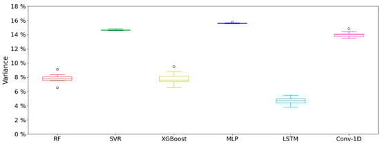
Figure 4.
Variance in the test set of the different models using k-fold method.
Figure 5 shows the dispersion and tendency of the forecast with respect to the actual values in the validation set. In contrast to the DL techniques, which are in the positive range, the ML architectures include instants in which the predictions are negative. This is because the validation set contains gaps to ensure the data continuity. These suffer from a slight inertia in the first learning epochs and are not capable of following the information provided by the data at the instants of change in which the signal is recovered. In general, a tendency can be observed for all models to overestimate low demand and underestimate high demand.
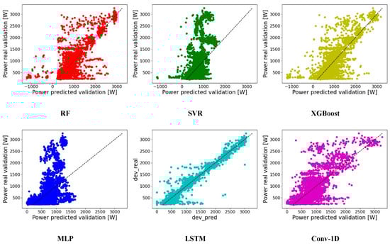
Figure 5.
Relationship intensity in the adjustment of the models in the validation set.
The MLP and SVR show a similar trend. Up to , they follow the patterns of the real data with a clear inclination to overestimate. Thereafter, they do not follow the trend and underestimate the electrical loads. There does not seem to be a significant improvement in the XGBoost forecast by adjusting the weak learners, since RF and XGBoost show a similar tendency. Not considering the negative values, these have a dispersion that tends to overestimate at low demand levels and overestimate at high levels. This same tendency can be observed in Conv-1D. The LSTM adequately follows the trend of the real data, although it presents moments with greater dispersion, mainly in the residual demands.
The dispersion and bias of the evaluated models in the test set is displayed in Figure 6. In contrast to what occurred in the validation set, the ML do not tend to falsify certain periods as missing values. The variation in the bias of the RF and XGBoost between the validation set (Figure 1) and test set (Figure 2), which changed from underestimate to overestimate, is due to this factor. As for the evaluation of the dispersion in the validation set, both models have a similar dispersion, without one model clearly standing out from the other. The SVR and the MLP have the same trend, with the MLP having more variance when it comes to predicting residual demands. When the electrical demand exceeds , neither of these two models is able to follow the real data patterns. The Conv-1D has a behavior similar to MLP causalities, with an even greater tendency to overestimate in low demand periods. In the case of powers above the range, unlike MLP, Conv-1D is capable of following the variations in demands with a certain dispersion. Except for residual demands, which LSTM tends to overestimate, this faithfully forecasts the patterns found in the real data.
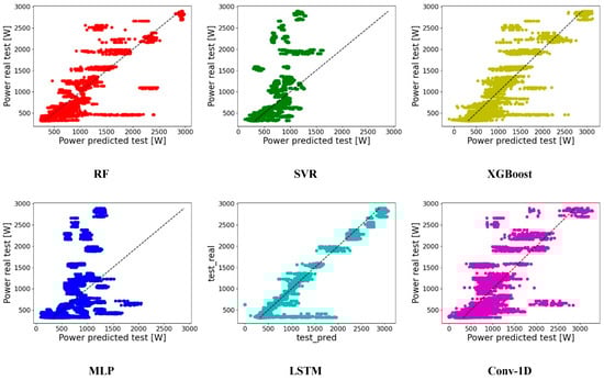
Figure 6.
Relationship intensity in the adjustment of the models in the test set.
The medians, quartiles and IQR of the error assessment metrics evaluated, i.e., , and , for the different models are displayed in Table 3. These values complement the figures presented throughout this section, reinforcing the comments with numerical values. The refers to the tendency of the models presented in Figure 1 and Figure 2. refers to the dispersion shown in Figure 3 and Figure 4 for the validation and test sets, respectively, in each pair. Both metrics are represented in Figure 5 (validation set) and Figure 6 (test set), which display the degree of interrelation between the results obtained and the real values.
Table 3.
Summary of error metrics in validation and test sets.
Table 3 shows the stability of the models constructed by testing them in different folds. The IQRs that are presented in both and in both splits show that the variability to the changes in the sets is reduced. Furthermore, looking at the changes in the median between the validation and the test set, it can be confirmed that the models are correctly fitted. In this way, knowing the test set as a set independent of training, i.e., where the quality of the modeling is evaluated under conditions different from those of the test, the reliability and reproducibility of the predictions made is guaranteed.
Observing the values obtained for the forecast that are presented in Table 3, it can be verified that the LSTM is the model that best adapts to the electrical demands. If is considered, the median is in the validation set and in the test set. The rest of the models are not able to adjust so well to the variable to be predicted. Evaluating the test set, i.e., independently of the training process set, the variance is 3% higher in the case of RF and XGBoost, and around 10% higher in the rest of the models. The bias, i.e., the tendency shown by the , is stable, showing slight variations in the adjustment of the models. The predictions show that possible variation in new datasets is reduced since the IQR is less than with most techniques.
The comparison of the adjustments in the different models built is graphically represented in Figure 7 for the validation sample, where a random cross-validation split was selected. As can be seen, the LSTM is the model that best fit the training sample. This, as expected, can adequately meet fluctuations in electrical loads in spite of it showing a slight underestimation in some periods when maximum demand occurs. The Conv-1D also has a good fit, although it seems to exhibit some anomalous behavior, for instance, in the fluctuations that appear on Wednesdays or not reaching peak levels during the day. As expected with the analysis of the metrics, RF and XGBoost have similar predictions, overestimating residual demands and not achieving a suitable adjustment to the variations in electrical loads. The worst settings are SVR and MLP. Nevertheless, SVR, is capable of reproducing part of the information to poorly meet the electrical loads pattern. The accumulation of inaccuracies observed in the SVR can be seen in the poor values in the metrics. On the other, because of the variability in the adjustment of MLP, its poor calibration does not stand out in the calculated metrics.
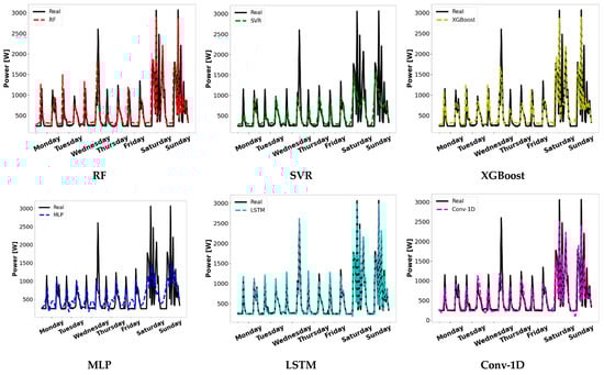
Figure 7.
Adjustment in validation sample in a random cross-validation split.
Figure 8 confirms the above comments about the superior performance of LSTM. This is the only model capable of faithfully reproducing the electrical loads on the testing sample. The main problem in RF and XGBoost seems to be the inability to accurately reproduce the residual demand values. Thus, these models underestimate these periods. This also occurs with Conv-1D, which still scarcely matches the real data fluctuations. As observed with the training sample, the SVR and MLP models performed worst in forecasting the electrical loads.
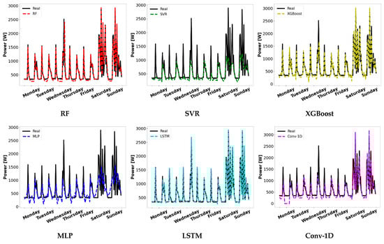
Figure 8.
Adjustment in test sample in a random cross-validation split.
6. Discussion
The substantial impact of the building sector on emissions of greenhouse gases means that adopting measures to meet sustainable development objectives is vital. The implementation of techniques to characterize fluctuations in the electrical loads enables better management of the energy needs in existing buildings. Thus, the comparative analysis of different AI techniques carried out in this paper provides a better understanding of the most appropriate models for forecasting electric power demand. The effective implementation of these techniques enables a more efficient and reliable energy system in buildings and can guide research in the field of ZEB.
Obtaining accurate electrical energy forecast models is key in the development of the building sector. Greater knowledge of electrical loads directly contributes to better use of energy since it allows greater control and a better response to the needs of buildings. The improvement in energy efficiency encourages facilities to adopt the necessary measures and facilitate the transition to the ZEB. Therefore, it offers the possibility of meeting the objectives set at a global level for reducing emissions.
In this paper, the models are constructed with missing values retained to preserve the continuity of the data. To compare results effectively, a seed is used. The performance of the models is obtained by analyzing their bias and variance in the validation and test samples. The reliability of the models is determined based on their ability to predict within a low from different sets obtained by a cross-validation technique. The adjustment that occurs between the predictions in the validation and test sets ensures the capability of the models to reproduce the results and their ability to forecast electrical loads.
There is not a linear relationship between the inputs considered to predict the electric energy since models with a more basic pattern extraction, such as MLP, fail to predict the objective variable. The inability shown by the SVR and MLP to predict variations in demand makes it impossible to use these models for the prediction of electricity consumption in buildings. All the models, except the LSTM, which has a slight tendency to overestimate the real values, show underestimation. In the case of adding human reasoning in post-processing, i.e., by invalidating the predictions with negative models of the ML values, it can be ensured that the RF and XGBoost follow the electrical patterns produced with a certain dispersion. The behavior of Conv-1d is similar to these models, despite there being slightly more variability. The performance obtained with LSTM makes it the most suitable model for the modeling and prediction of electricity consumption.
The forecast of the models in the test set is adjusted. Therefore, comparing the results with other similar analyses carried out recently, the performance shown in this study stands out. The accuracy shown (using nRMSE) in the less adjusted models, i.e., Conv-1D, SVR and MLP, is slightly higher, about 2%, than the models analyzed in [37,39]. The rest of the models analyzed, i.e., RF, XGBoost and LSTM, show a better performance than any of the models implemented in the aforementioned research. Therefore, in addition to the good fit offered by RF and SVR for the forecast of electrical loads, the superior performance of LSTM is clear.
The applied methodology offers a comprehensive comparison of different ML and DL models. The accuracy of the methods conducted is adequate, improving studies realized recently in the field of electricity consumption forecasting in buildings. As can be seen in the Results section, it is necessary to carry out a test method that considers the robustness of the models. In this way, the reliability of the results obtained can be analyzed.
The use of the nRMSE and nMBE metrics to determine the dispersion and trend of the predictions appears adequate to effectively categorize the evaluated models. Using these metrics and the adopted methodology, it is possible to determine the capacity of the models to reproduce the results obtained and the tendency of these models to overpredict or underpredict the data. Thus, by applying this methodology, the reproducibility and robustness of predictions in the future is ensured, i.e., in new datasets. Studies in the field of smart grids or local energy communities can benefit from the capacity of these models to effectively manage resources in buildings.
7. Conclusions
The impact of this research is related to the need to characterize electrical loads and act on them to improve building performance. This study can serve as the basis for an improvement in the analysis of smart buildings or smart grids to provide benefits such as optimizing distributed production, storage systems, and the presence of electric vehicles. The conclusions are summarized in the following points:
- The methodology used shows in detail the robustness and tendency of the studied models based on a comparative analysis in an effective and reliable manner.
- There is a trend suggesting that DL is better than ML, mainly due to the inclusion of missing values to conserve the data continuity.
- The performance of LSTM stands out with excellent results for predicting electrical loads, mainly because of the importance of the efficient modeling of the past input features, which in this study, were 6 h intervals.
- There is no improvement in using XGBoost over RF since these techniques seem to model the electric power demand in a similar way.
- The behavior of XGBoost, RF and Conv-1D is similar. Although they seem to follow the electric energy trends, they cannot be considered good predictors as they underestimate residual demands.
- The SNN, SVR have worse performance than LSTM.
The limitations of the research carried out are based on the need to generalize the study to different contexts. Different power profiles may require additional validation and adaptation. Also, the techniques employed have been developed on a limited subset of hyperparameters. The effectiveness of the models can vary according to the values used. Future work in the application of the advances obtained in this study could involve the integration of the techniques in a management system, the use of advanced architectures or the employment of real-time forecasting.
Author Contributions
Conceptualization, D.V. and M.C.-C.; methodology, M.C.-C.; software, M.C.-C. and M.M.-C.; validation, M.C.-C. and D.V.; formal analysis, M.C.-C. and S.R.; investigation, M.C.-C.; resources, D.V., P.E.-O. and S.R.; data curation, M.C.-C.; writing—original draft preparation, M.C.-C.; writing—review and editing, M.M.-C.; visualization, D.V.; supervision, P.E.-O. and S.R.; project administration, P.E.-O. and S.R.; funding acquisition, P.E.-O. All authors have read and agreed to the published version of the manuscript.
Funding
This work was supported by the Ministry of Science, Innovation and Universities of the Spanish Government (PV Smart project TED2021-130677B-I00 and the grant FPU19/01187), the Universidade de Vigo, Spain (grant 00VI 131H 6410211), and the European Group for territorial cooperation Galicia-North of Portugal (GNP, AECT) through the IACOBUS program of research stays.
Data Availability Statement
Data utilized in this manuscript can be found in References [45,46].
Conflicts of Interest
The authors declare no conflict of interest.
Nomenclature
| Preprocessing | |
| upper bound | |
| lower bound | |
| interquartile range | |
| third quartile | |
| first quartile | |
| RF section | |
| forecasted variable | |
| number of trees | |
| probability function of the forecasted variable given the independent variables | |
| objective function | |
| number of samples | |
| difficulty of each decision tree | |
| SVR section | |
| variance | |
| point being evaluated | |
| in the hyperplane | |
| slack margin of the SVR model | |
| number of independent variables | |
| hyperparameter that represents the regularization | |
| XGBoost section | |
| the iteration considered | |
| MLP section | |
| function of the studied neuron | |
| activation function of preceding neuron | |
| LSTM section | |
| kernel of the neuron connection | |
| bias of the neuron connection | |
| forget gate | |
| kernel of the forget gate | |
| bias of the forget gate | |
| information previously kept | |
| new data | |
| Information to be updated | |
| sequence regularized | |
| kernel of the phase of information retention of the input gate | |
| bias of the phase of information retention of the input gate | |
| kernel of the phase of sequence regulation of the input gate | |
| bias of the phase of sequence regulation of the input gate | |
| previous information kept in the cell state | |
| actual information of the cell state | |
| kernel of the information previously retained together with the new data | |
| bias of the information previously retained together with the new data | |
| activation function of the actual set of information | |
| activation function of the cell state | |
| Conv-1D section | |
| feature map | |
| input vector | |
| feature detector | |
| padding | |
| stride | |
| Performance evaluation section | |
| maximum value of the objective variable | |
References
- Deb, S.; Tammi, K.; Kalita, K.; Mahanta, P. Impact of electric vehicle charging station on distribution network. Energies 2018, 11, 178. [Google Scholar] [CrossRef]
- Ma, X.; Wang, S.; Li, F.; Zhang, H.; Jiang, S.; Sui, M. Effect of air flow rate and temperature on the atomization characteristics of biodiesel in internal and external flow fields of the pressure swirl nozzle. Energy 2022, 253, 124112. [Google Scholar] [CrossRef]
- Kakandwar, S.; Bhushan, B.; Kumar, A. Chapter 3—Integrated machine learning techniques for preserving privacy in Internet of Things (IoT) systems. In Blockchain Technology Solutions for the Security of IoT-Based Healthcare Systems; Academic Press: Cambridge, MA, USA, 2023; pp. 45–75. [Google Scholar] [CrossRef]
- Sheena, N.; Joseph, S.; Sivan, S.; Bhushan, B. Light-weight privacy enabled topology establishment and communication protocol for swarm IoT networks. Clust. Comput. 2022, in press. [Google Scholar] [CrossRef]
- International Energy Agency. Appliances and Equipment; International Energy Agency: Paris, France, 2020.
- Chauhan, R.K.; Chauhan, K. Building automation system for grid-connected home to optimize energy consumption and electricity bill. J. Build. Eng. 2019, 21, 409–420. [Google Scholar] [CrossRef]
- Yu, L.; Qin, S.; Zhang, M.; Shen, C.; Jiang, T.; Guan, X. A review of Deep Reinforcement Learning for smart building energy management. IEEE Internet Things J. 2021, 8, 12046–12063. [Google Scholar] [CrossRef]
- Thomas, D.; Deblecker, O.; Ioakimidis, C.S. Optimal operation of an energy management system for a grid-connected smart building considering photovoltaics’ uncertainty and stochastic electric vehicles’ driving schedule. Appl. Energy 2018, 210, 1188–1206. [Google Scholar] [CrossRef]
- European Commission. A European Long-Term Strategic Vision for a Prosperous, Modern, Competitive and Climate Neutral Economy; EU: Brussels, Belgium, 2018.
- International Energy Agency. Energy Efficiency 2018. Analysis and Outlooks to 2040; EU: Paris, France, 2018.
- Villanueva, D.; Cordeiro-Costas, M.; Feijoó-Lorenzo, A.E.; Fernández-Otero, A.; Míguez-García, E. Towards DC Energy Efficient Homes. Appl. Energy 2021, 11, 6005. [Google Scholar] [CrossRef]
- Xiong, R.; Cao, J.; Yu, Q. Reinforcement learning-based real-time power management for hybrid energy storage system in the plug-in hybrid electric vehicle. Appl. Energy 2018, 211, 538–548. [Google Scholar] [CrossRef]
- Tostado-Véliz, M.; Icaza-Alvarez, D.; Jurado, F. A novel methodology for optimal sizing photovoltaic-battery systems in smart homes considering grid outages and demand response. Renew. Energy 2021, 170, 884–896. [Google Scholar] [CrossRef]
- Nematchoua, M.K.; Marie-Reine Nishimwe, A.; Reiter, S. Towards nearly zero-energy residential neighbourhoods in the European Union: A case study. Renew. Sustain. Energy Rev. 2021, 135, 110198. [Google Scholar] [CrossRef]
- Brambilla, A.; Salvalai, G.; Imperadori, M.; Sesana, M.M. Nearly zero energy building renovation: From energy efficiency to environmental efficiency, a pilot case study. Energy Build. 2018, 166, 271–283. [Google Scholar] [CrossRef]
- Cordeiro-Costas, M.; Villanueva, D.; Eguía-Oller, P. Optimization of the Electrical Demand of an Existing Building with Storage Management through Machine Learning Techniques. Appl. Sci. 2021, 11, 7991. [Google Scholar] [CrossRef]
- Zhang, Q.; Yang, L.T.; Chen, Z.; Li, P. A survey on deep learning for big data. Inf. Fusion 2018, 42, 146–157. [Google Scholar] [CrossRef]
- Langer, L.; Volling, T. An optimal home energy management system for modulating heat pumps and photovoltaic systems. Appl. Energy 2020, 278, 115661. [Google Scholar] [CrossRef]
- Oh, S. Comparison of a Response Surface Method and Artificial Neural Network in Predicting the Aerodynamic Performance of a Wind Turbine Airfoil and Its Optimization. Appl. Sci. 2020, 10, 6277. [Google Scholar] [CrossRef]
- Thesia, Y.; Oza, V.; Thakkar, P. A dynamic scenario-driven technique for stock price prediction and trading. J. Forecast. 2022, 41, 653–674. [Google Scholar] [CrossRef]
- Runge, J.; Zmeureanu, R. Forecasting Energy Use in Buildings Using Artificial Neural Networks: A Review. Energies 2019, 12, 3254. [Google Scholar] [CrossRef]
- Habbak, H.; Mahmoud, M.; Metwally, K.; Fouda, M.M.; Ibrahem, M.I. Load Forecasting Techniques and Their Applications in Smart Grids. Energies 2023, 16, 1480. [Google Scholar] [CrossRef]
- López-Santos, M.; Díaz-García, S.; García-Santiago, X.; Ogando-Martínez, A.; Echevarría-Camarero, F.; Blázquez-Gil, G.; Carrasco-Ortega, P. Deep Learning and transfer learning techniques applied to short-term load forecasting of data-poor buildings in local energy communities. Energy Build. 2023, 292, 113164. [Google Scholar] [CrossRef]
- Madler, J.; Harding, S.; Weibelzahl, M. A multi-agent model of urban microgrids: Assessing the effects of energy-market shocks using real-world data. Appl. Energy 2023, 343, 121180. [Google Scholar] [CrossRef]
- Sethi, R.; Kleissl, J. Comparison of Short-Term Load Forecasting Techniques. In Proceedings of the 2020 IEEE Conference on Technologies for Sustainability (SusTech), Santa Ana, CA, USA, 23–25 April 2020. [Google Scholar] [CrossRef]
- Chou, J.S.; Tran, D.S. Forecasting energy consumption time series using machine learning techniques based on usage patterns of residential householders. Energy 2018, 165, 709–726. [Google Scholar] [CrossRef]
- Rafi, S.H.; Al-Masood, N.; Deeba, S.R.; Hossain, E. A Short-Term Load Forecasting Method Using Integrated CNN and LSTM Network. IEEE Access 2021, 9, 32436–32448. [Google Scholar] [CrossRef]
- Ye, Z.; Kim, M.K. Predicting electricity consumption in a building using an optimized back-propagation and Levenberg-Marquardt back-propagation neural network: Case study of a shopping mall in China. Sustain. Cities Soc. 2018, 42, 176–183. [Google Scholar] [CrossRef]
- Wang, C.; Baratchi, M.; Back, T.; Hoos, H.H.; Limmer, S.; Olhofer, M. Towards Time-Series Feature Engineering in Automated Machine Learning for Multi-Step-Ahead Forecasting. Eng. Proc. 2022, 18, 8017. [Google Scholar] [CrossRef]
- Fan, C.; Sun, Y.; Zhao, Y.; Song, M.; Wang, J. Deep learning-based feature engineering methods for improved building energy prediction. Appl. Energy 2019, 240, 35–45. [Google Scholar] [CrossRef]
- Tian, C.; Li, C.; Zhang, G.; Lv, Y. Data driven parallel prediction of building energy consumption using generative adversarial nets. Energy Build. 2019, 186, 230–243. [Google Scholar] [CrossRef]
- Dab, K.; Agbossou, K.; Henao, N.; Dubé, Y.; Kelouwani, S.; Hosseini, S.S. A compositional kernel based gaussian process approach to day-ahead residential load forecasting. Energy Build. 2022, 254, 111459. [Google Scholar] [CrossRef]
- Zeyu, W.; Yueren, W.; Rouchen, Z.; Srinivasan, R.S.; Ahrentzen, S. Random Forest based hourly building energy prediction. Energy Build. 2018, 171, 11–25. [Google Scholar] [CrossRef]
- Touzani, S.; Granderson, J.; Fernandes, S. Gradient boosting machine for modelling the energy consumption of commercial buildings. Energy Build. 2018, 158, 1533–1543. [Google Scholar] [CrossRef]
- Hadri, S.; Naitmalek, Y.; Najib, M.; Bakhouya, M.; Fakhiri, Y.; Elaroussi, M. A Comparative Study of Predictive Approaches for Load Forecasting in Smart Buildings. Procedia Comput. Sci. 2019, 160, 173–180. [Google Scholar] [CrossRef]
- Vrablecová, P.; Bou Ezzeddine, A.; Rozinajová, V.; Šárik, S.; Sangaiah, A.K. Smart grid load forecasting using online support vector regression. Comput. Electr. Eng. 2018, 65, 102–117. [Google Scholar] [CrossRef]
- Khan, S.; Javaid, N.; Chand, A.; Khan, A.B.M.; Rashid, F.; Afridi, I.U. Electricity Load Forecasting for Each Day of Week Using Deep CNN. Adv. Intell. Syst. Comput. 2019, 927, 1107–1119. [Google Scholar] [CrossRef]
- Chen, S.; Ren, Y.; Friedrich, D.; Yu, Z.; Yu, J. Prediction of office building electricity demand using artificial neural network by splitting the time horizon for different occupancy rates. Energy AI 2021, 5, 100093. [Google Scholar] [CrossRef]
- Amber, K.P.; Ahmad, R.; Aslam, M.W.; Kousar, A.; Usman, M.; Khan, M.S. Intelligent techniques for forecasting electricity consumption of buildings. Energy 2018, 157, 886–893. [Google Scholar] [CrossRef]
- Zhong, H.; Wang, J.; Jia, H.; Mu, Y.; Lv, S. Vector field-based support vector regression for building energy consumption prediction. Appl. Energy 2019, 242, 403–414. [Google Scholar] [CrossRef]
- Martínez-Comesaña, M.; Febrero-Garrido, M.; Granada-Álvarez, E.; Martínez-Torres, J.; Martínez-Mariño, S. Heat Loss Coefficient Estimation Applied to Existing Buildings through Machine Learning Models. Appl. Sci. 2020, 10, 8968. [Google Scholar] [CrossRef]
- Werner de Vargas, V.; Schneider Aranda, J.A.; dos Santos Costa, R.; da Silva Pereira, P.R.; Victória Barbosa, J.L. Imbalanced data preprocesing techniques for machine learning: A systematic mapping study. Knowl. Inf. Syst. 2023, 65, 31–57. [Google Scholar] [CrossRef]
- Ur Rehman, A.; Belhaouari, S.B. Unsupervised outlier detection in multidimensional data. J. Big Data 2021, 8, 80. [Google Scholar] [CrossRef]
- Bazlur Rashid, A.N.M.; Ahmed, M.; Pathan, A.K. Infrequent pattern detection for reliable network traffic analysis using robust evolutionary computation. Sensors 2021, 21, 3005. [Google Scholar] [CrossRef]
- Cordeiro-Costas, M.; Villanueva, D.; Eguía-Oller, P.; Granada-Álvarez, E. Machine Learning and Deep Learning Models Applied to Photovoltaic Production Forecasting. Appl. Sci. 2022, 12, 8769. [Google Scholar] [CrossRef]
- Xiong, Z.; Cui, Y.; Liu, Z.; Zhao, Y.; Hu, M.; Hu, J. Evaluating explorative prediction power of machine learning algorithms for materials discovery using k-fold forward cross-validation. Comput. Mater. Sci. 2020, 171, 109203. [Google Scholar] [CrossRef]
- Feng, Y.; Tu, Y. Phases of learning dynamics in artificial neural networks in the absence or presence of mislabeled data. Mach. Learn. Sci. Technol. 2021, 2, 043001. [Google Scholar] [CrossRef]
- Smith, G.D.; Ching, W.H.; Cornejo-Páramo, P.; Wong, E.S. Decoding enhancer complexity with machine learning and high-throughput discovery. Genome Biol. 2023, 24, 116. [Google Scholar] [CrossRef] [PubMed]
- Olu-Ajayi, R.; Alaka, H.; Owolabi, H.; Akanbi, L.; Ganiyu, S. Data-Driven Tools for Building Energy Consumption Prediction: A Review. Energies 2023, 16, 2574. [Google Scholar] [CrossRef]
- Ai, H.; Zhang, K.; Sun, J.; Zhang, H. Short-term Lake Erie algal bloom prediction by classification and regression models. Water Res. 2023, 232, 119710. [Google Scholar] [CrossRef]
- Park, H.J.; Kim, Y.; Kim, H.Y. Stock market forecasting using a multi-task approach integrating long short-term memory and the random forest framework. Appl. Soft Comput. 2022, 114, 1081106. [Google Scholar] [CrossRef]
- Roy, A.; Chakraborty, S. Support vector machine in structural reliability analysis: A review. Reliab. Eng. Syst. Saf. 2023, 233, 109126. [Google Scholar] [CrossRef]
- Alrobaie, A.; Krati, M. A Review of Data-Driven Approaches for Measurement and Verification Analysis of Building Energy Retrofits. Energies 2022, 15, 7824. [Google Scholar] [CrossRef]
- Pimenov, D.Y.; Dustillo, A.; Wojciechowski, S.; Sharma, V.S.; Gupta, M.K.; Kontoglu, M. Artificial intelligence systems for tool condition monitoring in machining: Analysis and critical review. J. Intell. Manuf. 2023, 34, 2079–2121. [Google Scholar] [CrossRef]
- Huang, K.; Guo, Y.F.; Tseng, M.L.; Wu, K.J.; Li, Z.G. A Novel Health Factor to Predict the Battery’s State-of-Health Using a Support Vector Machine Approach. Appl. Sci. 2018, 8, 1803. [Google Scholar] [CrossRef]
- Jassim, M.A.; Abd, D.H.; Omri, M.N. Machine learning-based new approach to films review. Soc. Netw. Anal. Min. 2023, 13, 40. [Google Scholar] [CrossRef]
- Yang, L.; Shami, A. IoT data analytics in dynamic environments: From an automated machine learning perspective. Eng. Appl. Artif. Intell. 2022, 116, 105366. [Google Scholar] [CrossRef]
- Priscilla, C.V.; Prabha, D.P. Influence of Optimizing XGBoost to Handle Class Imbalance in Credit Card Fraud Detection. In Proceedings of the 2020 Third International Conference on Smart Systems and Inventive Technology (ICSSIT), Tirunelveli, India, 20–22 August 2020; pp. 1309–1315. [Google Scholar] [CrossRef]
- Cao, J.; Gao, J.; Nikafshan Rad, H.; Mohammed, A.S.; Hasanipanah, M.; Zhou, J. A novel systematic and evolved approach based on XGBoost-firefly algorithm to predict Young’s modulus and unconfined compressive strength of rock. Eng. Comput. 2022, 38, 3829–3845. [Google Scholar] [CrossRef]
- Bienvenido-Huertas, D.; Sánchez-García, D.; Marín-García, D.; Rubio-Bellido, C. Analysing energy poverty in warm climate zones in Spain through artificial intelligence. J. Build. Eng. 2023, 68, 106116. [Google Scholar] [CrossRef]
- Qin, Y.; Luo, H.; Zhao, F.; Fang, Y.; Tao, X.; Wang, C. Spatio-temporal hierarchical MLP network for traffic forecasting. Inf. Sci. 2023, 632, 543–554. [Google Scholar] [CrossRef]
- Li, H.; Gao, W.; Xie, J.; Yen, G.G. Multiobjective bilevel programming model for multilayer perceptron neural networks. Inf. Sci. 2023, 642, 119031. [Google Scholar] [CrossRef]
- Lee, D.H.; Lee, D.; Han, S.; Seo, S.; Lee, B.J.; Ahn, J. Deep residual neural network for predicting aerodynamic coefficient changes with ablation. Aerosp. Sci. Technol. 2023, 136, 108207. [Google Scholar] [CrossRef]
- Panerati, J.; Schnellmann, M.-A.; Patience, C.; Beltrame, G.; Patience, G.-S. Experimental methods in chemical engineering: Artificial neural networks-ANNs. Can. J. Chem. Eng. 2019, 97, 2372–2382. [Google Scholar] [CrossRef]
- Marfo, K.F.; Przybyla-Kasperek, M. Study on the Use of Artificially Generated Objects in the Process of Training MLP Neural Networks Based on Dispersed Data. Entropy 2023, 25, 703. [Google Scholar] [CrossRef]
- Dai, C.; Wei, Y.; Xu, Z.; Chen, M.; Liu, Y.; Fan, J. ConMLP: MLP-Based Self-Supervised Contrastive Learning for Skeleton Data Analysis and Action Recognition. Sensors 2023, 23, 2452. [Google Scholar] [CrossRef]
- Zhao, R.; Yang, R.; Chen, Z.; Mao, K.; Wang, P.; Gao, R.-X. Deep learning and its applications to machine health monitoring. Mech. Syst. Signal Process. 2019, 115, 213–237. [Google Scholar] [CrossRef]
- Pal, P.; Chattopadhyay, P.; Swarnkar, M. Temporal feature aggregation with attention for insider threat detection from activity logs. Expert Syst. Appl. 2023, 224, 119925. [Google Scholar] [CrossRef]
- Sareen, K.; Panigrahi, B.K.; Shikhola, T.; Sharma, R. An imputation and decomposition algorithms based integrated approach with bidirectional LSTM neural network for wind speed prediction. Energy 2023, 278, 127799. [Google Scholar] [CrossRef]
- Laib, O.; Khadir, M.T.; Mihaylova, L. Toward efficient energy systems based on natural gas consumption prediction with LSTM Recurrent Neural Networks. Energy 2019, 177, 530–542. [Google Scholar] [CrossRef]
- Zhao, H.; Sun, S.; Jin, B. Sequential Fault Diagnosis Based on LSTM Neural Network. IEEE Access 2018, 6, 12929–12939. [Google Scholar] [CrossRef]
- Zaman, S.K.U.; Jehangiri, A.I.; Maqsood, T.; Umar, A.I.; Khan, M.A.; Jhanjhi, N.Z.; Shorfuzzaman, M.; Masud, M. COME-UP: Computation Offloading in Mobile Edge Computing with LSTM Based User Direction Prediction. Appl. Sci. 2022, 12, 3312. [Google Scholar] [CrossRef]
- Lablack, M.; Shen, Y. Spatio-temporal graph mixformer for traffic forecasting. Expert Syst. Appl. 2023, 228, 120281. [Google Scholar] [CrossRef]
- Ju, T.; Sun, G.; Chen, Q.; Zhang, M.; Zhu, H.; Rehman, M.U. A model combining convolutional neural network and lightgbm algorithm for ultra-short term wind power forecasting. IEEE Access 2019, 7, 28309–28318. [Google Scholar] [CrossRef]
- Zhang, Q.; Jin, Q.; Chang, J.; Xiang, S.; Pan, C. Kernel-Weighted Graph Convolutional Network: A Deep Learning Approach for Traffic Forecasting. In Proceedings of the 24th International Conference on Pattern Recognition (ICPR 2018), Beijing, China, 20–24 August 2018; pp. 1018–1023. [Google Scholar] [CrossRef]
- Mitra, S. Deep Learning with Radiogenomics towards Personalized Management of Gliomas. IEEE Rev. Biomed. Eng. 2023, 16, 579–593. [Google Scholar] [CrossRef]
- Borghesi, M.; Costa, L.D.; Morra, L.; Lamberti, F. Using Temporal Convolutional Networks to estimate ball possession in soccer games. Expert Syst. Appl. 2023, 223, 119780. [Google Scholar] [CrossRef]
- Velayuthapandian, K.; Subramoniam, S.P. A focus module-based lightweight end-to-end CNN framework for voiceprint recognition. Signal Image Video Process. 2023, 17, 2817–2825. [Google Scholar] [CrossRef]
- Goay, C.H.; Ahmad, N.S.; Goh, P. Temporal convolutional networks for transient simulation of high-speed channels. Alex. Eng. J. 2023, 74, 643–663. [Google Scholar] [CrossRef]
- Taqi, A.M.; Awad, A.; Al-Azzo, F.; Milanova, M. The Impact of Multi-Optimizers and Data Augmentation on TensorFlow Convolutional Neural Network Performance. In Proceedings of the 1st IEEE Conference on Multimedia Information Processing and Retrieval (MIPR 2018), Miami, FL, USA, 10–12 April 2018; pp. 140–145. [Google Scholar] [CrossRef]
- Zhang, J.; Lu, C.; Li, X.; Kim, H.J.; Wang, J. A Full Convolutional Network Based on DenseNet for remote sensing scene classification. Math. Biosci. Eng. 2019, 16, 3345–3367. [Google Scholar] [CrossRef] [PubMed]
- William, H.; Fanney, A.H.; Dougherty, B.; Payne, W.V.; Ullah, T.; Ng, L.; Omar, F. Net Zero Energy Residential Test Facility Instrumented Data; Year 2. 2017. Available online: https://pages.nist.gov/netzero/data.html (accessed on 3 July 2023).
- William, H.; Chen, T.H.; Dougherty, B.; Fanney, A.H.; Ullah, T.; Payne, W.V.; Ng, L.; Omar, F. Net Zero Energy Residential Test Facility Instrumented Data; Year 1. 2018. Available online: https://pages.nist.gov/netzero/ (accessed on 3 July 2023).


Disclaimer/Publisher’s Note: The statements, opinions and data contained in all publications are solely those of the individual author(s) and contributor(s) and not of MDPI and/or the editor(s). MDPI and/or the editor(s) disclaim responsibility for any injury to people or property resulting from any ideas, methods, instructions or products referred to in the content. |
© 2023 by the authors. Licensee MDPI, Basel, Switzerland. This article is an open access article distributed under the terms and conditions of the Creative Commons Attribution (CC BY) license (https://creativecommons.org/licenses/by/4.0/).