Abstract
This paper presents an optimization method that aims to mitigate disturbances in the radial-feed system of the ring-pendulum double-sided polisher (RDP) during processing. We built a radial-feed system model of an RDP and developed a single-tube robust model predictive control system to enhance the disturbance rejection capability of the radial-feed system. To constrain the system states inside the terminal constraint set and further enhance the system’s robustness, we added the ε-approximation to approach the single-tube terminal constraint set. Finally, the effectiveness of the proposed method for the RDP radial-feed system was verified through simulations and experiments. These findings demonstrate the potential of the proposed method for improving the performance of the RDP radial-feed system in practical applications. The polish processing results demonstrated a substantial improvement in the accuracy of the surface shape measurements obtained by applying the STRMPC method. Compared to the MPC method, the PV value decreased from 1.49 λ PV to 0.99 λ PV, indicating an improvement in the convergence rate of approximately 9.78%. Additionally, the RMS value decreased from 0.257 λ RMS to 0.163 λ RMS, demonstrating a remarkable 35.6% enhancement in the convergence rate.
1. Introduction
The ring-pendulum double-sided polisher (RDP) is a high-precision optical processing machine. It is designed for processing large-aperture planar optical components. These components are widely used in various essential scientific and technological fields, including space telescopes [1,2,3], high-energy laser weapons [4,5,6], laser nuclear fusion systems [7], and other essential scientific and technological fields [8,9,10].
In order to improve the precision optical element processing, numerous amounts of research have been carried out.
Numerous studies have been conducted to enhance precision optical element processing. Zhong et al. [11] systematically investigated the effects of four crucial process factors, namely polish pressure, pad rotational speed, polish head rotational speed, and slurry supply velocity, on chemically mechanically polished optical silicon substrates. Through meticulous CMP experiments, they successfully identified the optimal combination of these factors, resulting in a significant improvement in polishing efficiency. Ban et al. [12] introduced an advanced conditioning method called subaperture conditioning. By strategically removing and controlling specific regions of the pad surface using a smaller-sized conditioner tool, this method achieves a more uniform surface shape and higher polishing accuracy. Zhao et al. [13] investigated a polished trajectory interpolation scheme to ensure accuracy in trajectory runtime. The NURBS interpolation approach demonstrated a remarkable improvement in both interpolation and runtime error compared to linear interpolation. Moreover, the convergence rate of surface error for elements improved from 37.59% to 44.44%. Pirayesh et al. [14] examined the influence of slurry pH on the size of silica abrasives and their colloidal stability, and how these factors ultimately impacted the polish rate. Their findings provided strong evidence supporting the significant effects of slurry pH, abrasive concentration, and grain size on the polish rate. Notably, smaller abrasive particles with higher surface area showed improved performance in terms of polish rate. Chen et al. [15] investigated the impact of robot motion accuracy on element surface topography during polishing. They developed a material removal model that considers the normal error of the polishing tool, enabling predictions of surface morphology and form accuracy under varying normal-error conditions. This model offers guidance for achieving uniform material removal and improving polishing accuracy. Zhang et al. [16] proposed a material removal model to reduce surface roughness of optical elements. Through systematic analysis, they established a uniform polishing method that efficiently enhanced the surface roughness of hard-polished spherical optics. Zhang et al. [17] developed a material-removing model to analyze the effects of rotary table run-out error on polishing efficiency and accuracy at any given point on the element. Through an analysis and a series of polishing experiments using the KPJ1700 and KPJ1200 CMP machines, they obtained definitive evidence that reducing the run-out error leads to improved polishing efficiency and accuracy. Huang et al. [18] introduced an interpolation process for polishing trajectory using the equal proportional feed rate adjustment strategy. This approach significantly improved the accuracy of implementing dwell time in optical polishing. Simulations and experiments demonstrated that their proposed dwell time algorithm and spline interpolation method had a notable impact on enhancing the solution accuracy of dwell time and improving the convergence rate of form error during the polishing process.
These studies have led to significant advances in improving the accuracy and efficiency of the polishing process through the optimization of the process and the construction of material removal models from various perspectives. However, the uncertainty disturbances during the machining process can affect the polishing efficiency and the precision of the processed optical elements. Therefore, the disturbance rejection control of the RDP’s radial-feed system requires further investigation.
Various control methods, such as proportional-integral-derivative (PID) control [19,20,21], sliding mode control [22,23,24], and model predictive control (MPC) [25,26,27,28], are commonly used in practical systems. PID control is known for its simplicity and ease of implementation, effectively suppressing small disturbances. However, its performance may be compromised when facing complex uncertainty perturbations. Sliding mode control excels at attenuating uncertainties but may introduce significant control oscillations, posing challenges in applications. MPC demonstrates excellent disturbance rejection capabilities by optimizing control actions based on a predictive model to minimize future errors. Despite its strengths in handling disturbances, MPC has limitations when dealing with substantial interferences that exceed the predictive model’s capabilities. In comparison, robust model predictive control (RMPC) offers superior disturbance rejection capabilities [29,30,31,32,33,34]. By considering system uncertainties and employing robust optimization techniques, RMPC enhances its ability to withstand disturbances. However, it is important to note that even RMPC may have limitations when confronted with significant interferences, necessitating additional considerations during implementation.
This paper proposes an optimization method for the polishing process. The proposed method focuses on improving the radial-feed speed accuracy by establishing a single-tube RMPC system for the radial-feed system. By effectively mitigating disturbances during processing, this control system significantly enhances the performance of the radial-feed speed control in the RDP, resulting in improved polishing efficiency and accuracy for the RDP.
The subsequent sections of this paper are structured as follows. This paper is organized as follows. In Section 2, we establish the model for the radial-feed system of the RDP. In Section 3, we conduct the control structure of the RDP radial-feed system, highlighting the design of the single-tube robust model predictive control system. In Section 4, we present simulations and experiments that validate the effectiveness of our proposed method. Section 5 concludes the whole paper.
2. Model of Radial-Feed System of the RDP
The RDP is presented in Figure 1. It mainly comprises the lower-polishing disk with rotation pedestal, the element fixation disk, and the upper-polishing disk. The optical element is positioned on the element fixation disk, and the lower-polishing disk polishes the lower surface through rotation. The upper disk and the element-fixation disk polish the optical element’s upper surface by rotational and radial-feed motion simultaneously.
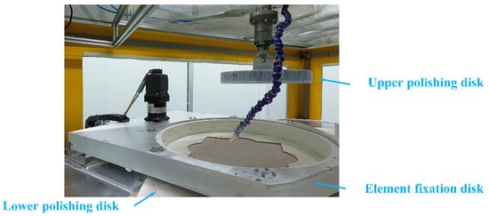
Figure 1.
The ring-pendulum double-sided polisher.
The radial-feed motion of the element fixation disk is less susceptible to uncertain disturbances compared to that of the upper-polishing disk. We establish a model for the radial-feed system of the latter. The upper-polishing disk radial-feed system of the RDP’s structure is demonstrated in Figure 2. The radial-feed system is composed of a radial-feed permanent-magnet synchronous motor, a spherical screw drive, and an upper-polishing disk. The screw is driven by the motor to realize the radial-feed motion.
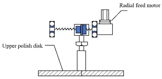
Figure 2.
Schematic diagram of radial-feed system of ring pendulum double-sided polisher.
The second-order system model proposed in Equation (1) represents an open-loop transfer function of the radial feed’s speed and current. The motor driving current provides the input, while the radial-feed motor speed of the upper-polishing disk represents the output. The remaining physical quantities in Equation (1) have the following meanings: is the load torque, is the number of motor poles, is the flux of a permanent magnet, is the motor’s moment of inertia, and is the viscous damping coefficient.
Equation (2) shows the radial-feed system model with its parameters identified by the multi-innovation stochastic gradient descent parameter identification method [35,36].
To facilitate the subsequent controller design, we transform the system transfer function into the state space in Equation (3), which adds the interferences of the system state and control quantity into the model.
where A = [0.0788, −0.1852; 1.0000, 0], B = [1; 0], and C = [−2.0491, 88.5127]. is the system state variable and is the system control quantity. and are system state disturbance and control quantity disturbance, respectively.
3. RDP Radial-Feed System Control Structure
3.1. Single-Tube RMPC
Figure 3 shows the control structure of the single-tube RMPC. is the actual input. is the actual output. The difference between the input and output is defined as actual state .
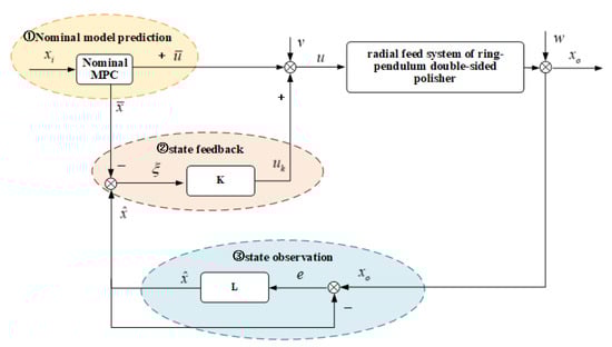
Figure 3.
Single-tube RMPC structure.
The structure consists of three parts: nominal model predictive control, state estimation, and state feedback. The identification system model is utilized for the nominal MPC optimization. represents the estimated state of the system, which is obtained through the utilization of the estimation matrix L. The total control volume of the single-tube robust predictive controller consists of the nominal model predictive control (MPC) and the feedback control. Moreover, the system state gradually approaches the origin under the influence of the control quantity.
, , , and in Equation (3) are constrained by Equation (4). , , , and represent the constraint sets containing the origin. Equation (5) describes the nominal MPC system, which excludes the disturbances and . is the nominal prediction state . is the nominal model prediction control quantity.
is a sequence of the nominal system state and is a sequence of the optimal control quantity at k = [0,… k]. The integer N represents the prediction horizon length. At current time k, is the nominal MPC system state and is the nominal MPC control quantity. represents the nominal MPC reachable set, while R and Q are two weight matrices in nominal MPC cost function .
The feedback matrix K can eliminate the distance between the actual state and the estimated state. To ensure system stability, the feedback matrix K must satisfy the condition that the spectral radius of matrix is below a value of 1.
in Equation (9) is the estimated state. The parameters in estimated matrix L must guarantee that the spectral radius of matrix is below a value of 1, ensuring system stability. The estimated error is defined as the difference between and . The prediction error is defined as the difference between and .
Combining Equations (11) and (12), the actual state can be presented as follows:
Combining Equations (7)–(12), we obtained the error system as follows:
is the Minkowski sum in the following formulas, where represents the operation symbol. The terminal constraint set for and is designed by utilizing the minimal robust invariant set. According to Equations (14)–(16), we can obtain the constraint set for and the constraint set for .
Combining the calculation of minimal robust invariant set in Reference [37] and Equations (14) and (15), we can obtain the minimal robust invariant sets and .
3.2. ε- Approximation of the Single-Tube Terminal Constraint Set
This section presents the computation of the single-tube terminal constraint set and approximates it by utilizing the ε-approximation method.
We define the single-tube constraint variable as . According to Equations (14)–(17), we obtain the calculation formulas of single-tube constraint reduction:
In order to extend the allowable range of system disturbances, the ε-approximation is designed for the single-tube terminal constraint set. We can utilize the following formula to calculate the single-tube constraint set .
For scalars and ε > 0, there exists a positive integer s that satisfies the condition , which further satisfies . Then, we define as the ε-approximation of .
When , Equation (22) and hold, so that and . Based on Equations (24) and (25), can approach , when we choose appropriate s or α.
Equation (26) shows that when condition holds, , and where represents a p-norm ball in , then is an -approximation of the minimal robust invariant set .
Table 1 presents an overview of the single-tube RMPC structure, which involves an offline computation phase and online computation phase. Steps 1 and 2 involve the former, while steps 3 and 4 are related to the latter. Step 2 computes , which is utilized to constrain the system state. The control quantity in step 4 facilitates the system state gradual convergence towards zero. For a more comprehensive understanding of the STRMPC control process, Figure 4 provides a visual representation.

Table 1.
Steps of RDP radial-feed system control method.
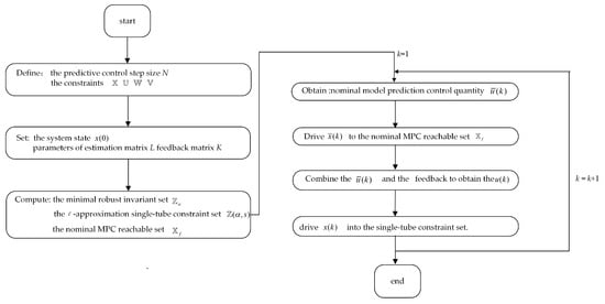
Figure 4.
Flowchart of RDP radial-feed system control method.
3.3. Stability Analysis
As part of our analysis, we prove that the nominal MPC shows recursive feasibility. Moreover, we prove that will be contained in the terminal constraint set and eventually approach zero.
Using Equation (6), we obtain the difference between the nominal predictive optimization cost functions and as follows:
Then, by combining Equation (27) and the condition , we obtain:
The inequality of nominal model prediction optimization cost functions is extended as:
Due to the nominal MPC ignoring the uncertain disturbance, we demonstrate that is a bounded and non-increasing sequence; therefore, the nominal MPC shows recursive feasibility.
As the nominal MPC shows recursive feasibility, when , , and are satisfied, and . Then, using Equation (23), we can obtain , . For , we can derive from ; for , is satisfied. When , we can obtain ; then, . As condition , the system state is asymptotically stable. The system states will gradually approach zero and stabilize in the .
4. Simulation and Experiment Verification
The parameters of single-tube RMPC (STRMPC) are as follows:
The constraints of the radial-feed control system state variable and its acceleration are defined as , the constraint of the system input control quantity current is , the constraint of the state disturbance is , and the constraint of the control disturbance is .
The nominal MPC parameters for the STRMPC are as follows:
The matrices Q = [1, 0; 0, 1] and R = [0.01]. The observation matrix is set as L = [0.0022; 0.0023]. The feedback matrix is set as K = [−0.0372, 0.0882] and the prediction horizon length is N = 15. The MPC method is provided as a comparison to the proposed method. The parameters of the matrices K, Q, and R in the MPC are identical to those in the nominal MPC.
As outlined in Section 3, the off-line calculation phase involved simulating the proposed algorithm and the MPC method to evaluate their performance, including a comprehensive analysis of the calculation costs. These simulations were conducted using MATLAB (R2019b) software on a computer system comprising an Intel Core i7–9750H CPU and 8 GB RAM. During the off-line computation phase, the MPC method exhibited a computation time of 0.54s, whereas the STRMPC method required a slightly longer duration of 0.79 s. The slightly longer computation time of the proposed method during the off-line calculation phase does not affect the subsequent simulations and experiments outlined in this study, as these calculations are performed in advance.
4.1. Simulation
We set step, sine, and square wave with amplitudes of 10 rpm and periods of 16 s as input signals. We separately added noise and load disturbances to the system output to validate the proposed method’s disturbance rejection capability. The initial system states for the STRMPC and MPC were defined as . We used the integral of the time-weighted absolute error (ITAE) performance index to evaluate the control performance.
(1) Load disturbance
To verify the system disturbance rejection performance with load disturbance, we superimposed a 1 rpm load disturbance onto the system output at 16 s and computed the ITAE indices.
In Figure 5, is presented on the horizontal axis as the system state and is presented on the vertical axis as the derivative of the system state. The green patches in Figure 5 represent the single-tube terminal constraint set , while the gray patches denote the nominal MPC reachable set . The convergence results shows that the actual system state follows and , then eventually converges within the single-tube constraint set.
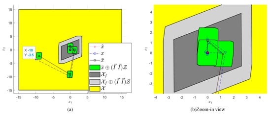
Figure 5.
Convergence of system state and terminal constraint set with load disturbance.
Figure 6, Figure 7 and Figure 8 show that the output curve without a controller is unable to resist the load disturbance. However, the MPC control method is able to resist load disturbance but still produces an overshoot. In comparison, the proposed method efficiently suppresses the disturbance and rarely produces an overshoot.
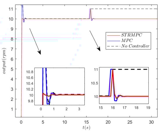
Figure 6.
Step response with load disturbance.
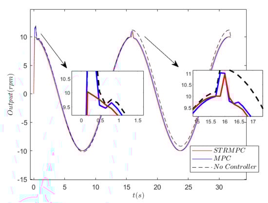
Figure 7.
Sine wave tracking with load disturbance.
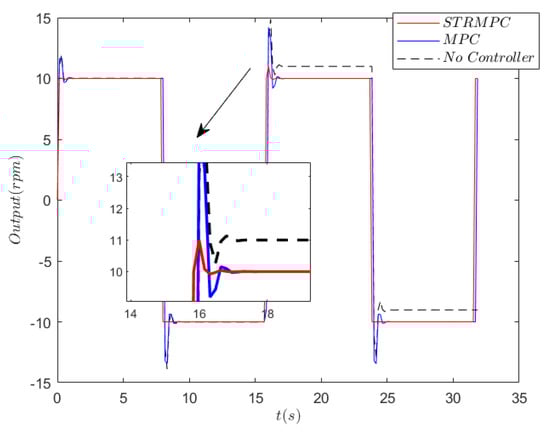
Figure 8.
Square wave tracking with load disturbance.
Table 2 presents the ITAE indices obtained from the simulations. The STRMPC method achieves an ITAE index of 1.9203 in square wave tracking, which is approximately 89.87% lower than the MPC method and 94.63% lower than the no controller method. Similarly, for sine wave tracking and step response, the ITAE index of the STRMPC method is also 83.87% and 30.79% lower than the MPC method and 91.87% and 90.13% lower than the no controller method, respectively. The STRMPC method achieves higher control effectiveness compared to MPC and no controller. Compared with the results of the no controller and MPC method, the proposed STRMPC method has the smallest ITAE index, which indicates that the STRMPC method has better control performance.
Table 2.
ITAE indices with load disturbance.
(2) Noise disturbance
The random white noise disturbance with the amplitude range of [−0.5, 0.5] is set as the noise interference.
From Figure 9, the STRMPC method is able to maintain in a terminal constraint set. Figure 10, Figure 11 and Figure 12 demonstrate that the proposed STRMPC method is more effective in suppressing noise disturbance compared to the MPC method. Based on the simulation results in Table 3, it can be observed that the STRMPC method demonstrates higher control efficiency compared to the other methods. In square wave tracking, the STRMPC method has an ITAE index of 4.3713, which is approximately 83.29% lower than the MPC method and 84.86% lower than the no controller method. Similarly, for sine wave tracking and step response, the ITAE index of the STRMPC method is lower than the other two methods. It shows that the proposed method has the lowest index value, which also demonstrates its stability and tracking accuracy.
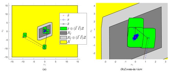
Figure 9.
Convergence of system state and terminal constraint set with ± 0.5 noise disturbance.
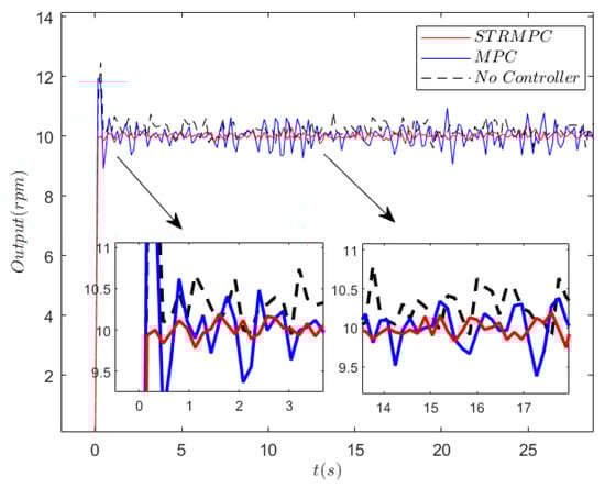
Figure 10.
Step response with ±0.5 noise disturbance.
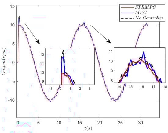
Figure 11.
Sine wave tracking with ±0.5 noise disturbance.
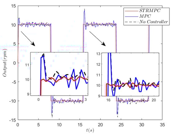
Figure 12.
Square wave tracking with ±0.5 noise disturbance.
Table 3.
ITAE indices with ±0.5 noise.
To further verify the noise suppression capability of the proposed method, we expanded the noise range to [−1, 1]. The simulation results are presented below.
From Figure 13 it can be seen that the system actual states remain within the terminal constraint set. Therefore, this simulation result indicates that increasing noise interference has a rare effect on the system stability of the STRMPC method.
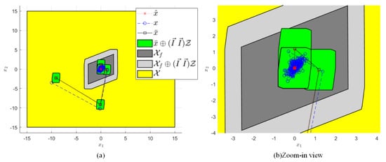
Figure 13.
Convergence of system state and terminal constraint set with ±1 noise disturbance.
Figure 14, Figure 15 and Figure 16 show the ability of the STRMPC method to effectively suppress the noise disturbance. The ITAE indices in Table 4 show that the STRMPC has a lowest value, indicating higher control accuracy compared to the other methods. The results demonstrate that the proposed method effectively suppresses interference, even in the presence of increased noise interference.
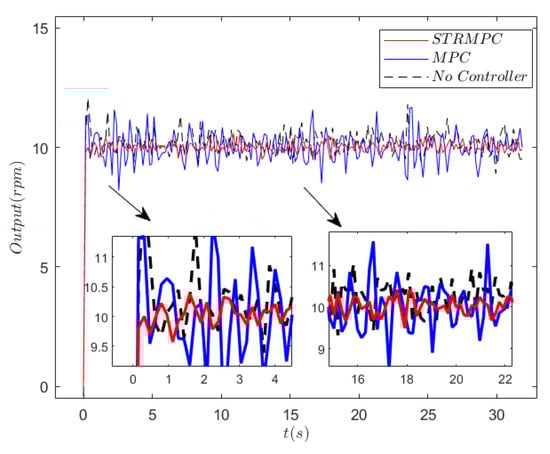
Figure 14.
Step response with ±1 noise disturbance.
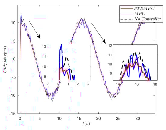
Figure 15.
Sine wave tracking with ±1 noise disturbance.
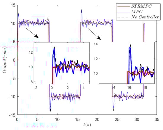
Figure 16.
Square wave tracking with ±1 noise disturbance.
Table 4.
ITAE indices with ±1 noise.
(3) Model parameters uncertainty
To verify the system robustness, we designed a model parameters uncertainty simulation with ±0.5 noise disturbance and load disturbance for the step response. The models with ±10% parameter fluctuations are laid out in Table 5.
Table 5.
Comparison of the model parameters.
The step response results in Figure 17, Figure 18, Figure 19 and Figure 20 show that the output of different models is nearly identical and that the model parameters uncertainty has little influence on the system performance. The results in Table 6 demonstrate that the STRMPC method exhibits high control effectiveness and robustness against model parameter fluctuations, load changes, and noise interference. The ITAE index remains relatively stable for the load disturbance test, with a maximum value increase of only 0.1359 from f1 to f5. Similarly, for the noise interference test, the ITAE index shows minimal increase, with a maximum value increase of only 0.1255 from f1 to f5. These results highlight the ability of the STRMPC method to maintain accurate control performance, demonstrating its robustness and effectiveness in achieving high-precision control.
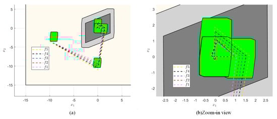
Figure 17.
Convergence of system state and terminal constraint set with ±1 noise disturbance.
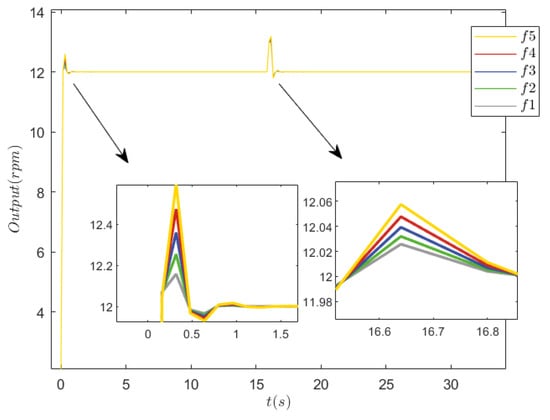
Figure 18.
Step response of different models with load disturbance.
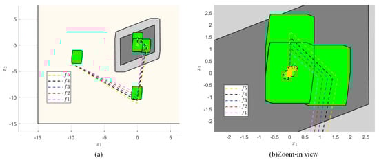
Figure 19.
Convergence of system state and terminal constraint set of different models with ± 0.5 noise disturbance.
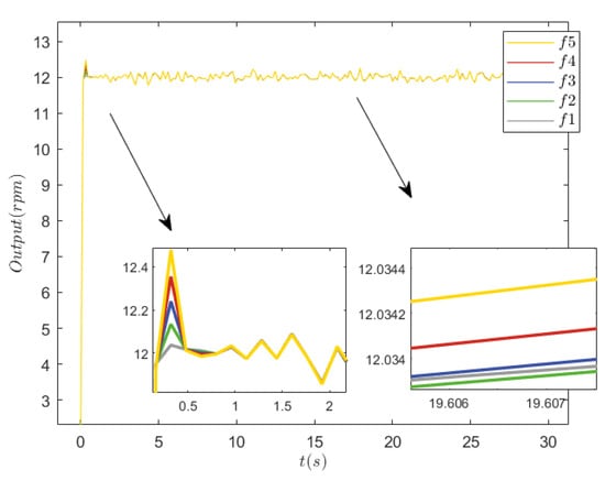
Figure 20.
Step response of different models with ±0.5 noise disturbance.
Table 6.
ITAE indices with ±1 noise.
Based on the simulation results on disturbance rejection and robustness, we conclude that the proposed STRMPC method exhibits extraordinary ability in suppressing noise and load disturbances, thereby demonstrating its robustness.
4.2. Experiment
To evaluate the effectiveness of the proposed method, we conducted experiments on the radial-feed motor speed and actual polishing process using MPC and STRMPC methods.
(4) Radial-feed motor speed
During the experiment on radial-feed motor speed, the sampling period was set to 0.002 s, and the radial-feed motor speed of the system with MPC method and system with no controller were given as comparisons to the proposed method. The radial-feed motor speed was set to 30 rpm, and, after the speed stabilized, we changed the reference to 18 rpm at a time of 20.84 s. The experiment’s results are present in Figure 20 and Figure 21.
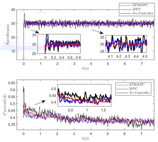
Figure 21.
Step response of the RDP radial-feed system [ref. speed = 30 rpm].
The experimental results indicate that the STRMPC displays outstanding robustness in Figure 21; the speed of the system with STRMPC has fewer steady errors than the speed outputs of comparison, and hardly produces the overshoot. The better control performance can be attributed to the STRMPC’s capability to restrict the output error through the single-tube terminal constraint set, as confirmed by the simulation results. The current curve in Figure 20 also verifies the robustness of the proposed method. Figure 22 demonstrates that when the speed changes abruptly, the proposed method has the more stable speed curves, which reflects its advantage in terms of robustness.
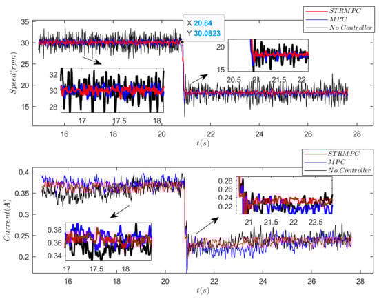
Figure 22.
Step response of the RDP radial-feed system [ref. speed = 30 rpm and 18 rpm].
(5) Actual polishing process
In the surface processing experiment, we chose a fused silica optical glass with dimensions of 430 × 430 mm and a thickness of 10 mm. The polishing pressure was set at 200 N, and the upper polishing disk had a radial displacement range of 20 mm relative to the center of the fused silica optical glass. Both the polishing disk and the glass were rotated at a speed of 15 rpm. Each piece of fused silica optical glass was then polished for a duration of 30 min. Surface shape detection was performed before and after processing; the peak-to-valley (PV) and root-mean-square (RMS) indices are presented in Figure 23 and Figure 24.
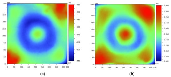
Figure 23.
Surface shape processing by STRMPC: (a) surface shape before processing [PV = 1.49 λ, RMS = 0.257 λ]; (b) surface shape after processing [PV = 0.99 λ, RMS = 0.163 λ].
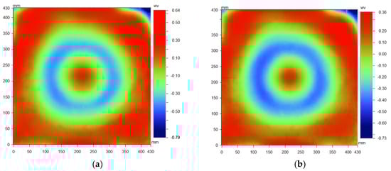
Figure 24.
Surface shape processing by MPC: (a) surface shape before processing [PV = 1.43 λ, RMS = 0.218 λ]; (b) surface shape after processing [PV = 1.09 λ, RMS = 0.216 λ].
The application of the MPC method yielded a 23.78% improvement in surface shape as evidenced by the reduction of the PV value from 1.43 λ to 1.09 λ. However, the reduction of RMS was reduced slightly from 0.218 λ RMS to 0.216 λ RMS, with a convergence rate of 0.9%. In contrast, the STRMPC method significantly enhanced both surface shape and roughness, reducing PV and RMS values from 1.49 λ PV and 0.257 λ RMS to 0.99 λ PV and 0.163 λ RMS, respectively. Compared with the MPC method, the STRMPC method achieved a higher convergence rate 33.56% and 36.57% for both PV and RMS. Specifically, the PV convergence rate was improved by 9.78%, while the RMS convergence rate increased by 35.6%. These findings suggest that the STRMPC method is more effective in improving surface shape and roughness accuracy than the conventional MPC method. Therefore, the STRMPC method’s stable radial feed enables rapid and stable processing of the ring-pendulum double-sided polisher, resulting in a more uniform surface shape.
5. Conclusions
In this paper, we propose a single-tube RMPC method for the RDP’s radial-feed system. The actual parameter identification model of the radial-feed system is presented. The single-tube RMPC structure is built to improve the disturbance suppression ability of the system. Further, the ε-approximation is conducted to enlarge the single-tube constraint sets, which improves the robustness of the system. Additionally, the stability analysis of the system is presented. Finally, the simulations and experiments have verified the efficacy of the proposed method in validating the disturbance rejection ability in the radial-feed system of RDP, and the uniformity of surface shape on optical elements processed by the RDP. Compared to the MPC method, the STRMPC method achieved higher convergence rates, a 9.78% improvement in PV convergence rate, and a 35.6% improvement in RMS convergence rate. These results demonstrate the superior performance of the STRMPC method in achieving faster and more accurate surface shape and roughness optimization.
However, this study includes the focus only on optimizing the radial-feed system motor speed control of the RDP, without focusing on its polish rotation system motor speed control. In the next step, the proposed method can be applied to rotation systems to achieve dual system linkage control, which further improves the polish efficiency and polish accuracy of the RDP.
Author Contributions
S.L.: Methodology, Writing—original draft. B.X.: Writing—review and editing. C.W.: Project administration, Funding acquisition. L.W.: Visualization. Z.W.: Validation. All authors have read and agreed to the published version of the manuscript.
Funding
This research was funded by the Equipment Advance Research Field Foundation, grant number: 80923010202.
Data Availability Statement
Data underlying the results presented in the paper are not publicly available at this time but may be obtained from the authors upon reasonable request.
Conflicts of Interest
The authors declare that there are no conflicts of interests; we do not have any possible conflicts of interest.
References
- Hugot, E.; Ferrari, M.; Hadi, K.E.; Vola, P.; Hubin, N. Active Optics: Stress polishing of toric mirrors for the VLT SPHERE adaptive optics system. Appl. Opt. 2009, 48, 2932–2941. [Google Scholar] [CrossRef]
- Zhao, W.; Wang, X.; Liu, H.; Lu, Z.; Lu, Z. Development of space-based diffractive telescopes. Front. Inf. Technol. Electron. Eng. 2020, 21, 884–902. [Google Scholar] [CrossRef]
- Qu, Y.; Jiang, Y.; Feng, L.; Li, X.; Liu, B. Lightweight design of multi-objective topology for a large-aperture space mirror. Appl. Sci. 2018, 8, 2259. [Google Scholar] [CrossRef]
- Zhan, R.; Lyu, C. Stop model development and analysis of optical collimation system for tactical high-energy laser weapon. Appl. Opt. 2021, 60, 3596–3603. [Google Scholar] [CrossRef]
- Sprangle, P.; Hafizi, B.; Ting, A.; Fischer, R. High-power lasers for directed-energy applications. Appl. Opt. 2015, 54, F201. [Google Scholar] [CrossRef]
- Nosov, P.A.; Shirankov, A.F.; Khorokhorov, A.M.; Zaytsev, K.I.; Yurchenko, S.O. Investigation of heating of optical elements during formation of high-power CW fiber laser radiation. Russ. Phys. J. 2019, 61, 2305–2312. [Google Scholar] [CrossRef]
- Derkach, I.N.; Kudryashov, E.A.; Kachalin, G.N.; Kirdyaev, N.A.; Ladeishchikova, V.V.; Timaev, D.S. Damage of dusty optical elements in the field of continuous-wave laser radiation. JETP Lett. 2018, 108, 379–383. [Google Scholar] [CrossRef]
- Xu, L.B.; Lu, X.Q.; Lei, Z.M. Influence of phase error of optical elements on optical path design of laser facilities. Acta Phys. Sin. -Chin. Ed. 2018, 67, 024201. [Google Scholar] [CrossRef]
- Sun, X.; Zhang, X.; Liu, Z.; Fan, Q.; Liu, C.; Zhu, J. Stress and wavefront measurement of large-aperture optical components with a ptychographical iterative engine. Appl. Opt. 2022, 61, 7231–7236. [Google Scholar] [CrossRef]
- Liu, Y.Q.; Ren, Z.; Shu, Y.; Wu, L.; Sun, J.; Cai, H.; Zhang, X.; Lu, L.; Qi, K.; Li, L.; et al. Broadband, large-numerical-aperture and high-efficiency microwave metalens by using a double-layer transmissive metasurface. Appl. Phys. Express 2021, 15, 014003. [Google Scholar] [CrossRef]
- Zhong, Z.W.; Tian, Y.B.; Ang, Y.J.; Wu, H. Optimization of the chemical mechanical polishing process for optical silicon substrates. Int. J. Adv. Manuf. Technol. 2012, 60, a12. [Google Scholar] [CrossRef]
- Ban, X.; Zhao, H.; Zhu, X.; Zhao, S.; Xie, R.; Liao, D. Improvement and application of pad conditioning accuracy in chemical mechanical polishing. Opt. Eng. 2018, 57, 095102-1. [Google Scholar] [CrossRef]
- Zhao, D.; Guo, H. A trajectory planning method for polishing optical elements based on a non-uniform rational b-spline curve. Appl. Sci. 2018, 8, 1355. [Google Scholar] [CrossRef]
- Pirayesh, H.; Cadien, K. The Effect of Slurry Properties on the CMP Removal Rate of Boron Doped Polysilicon. ECS J. Solid State Sci. Technol. 2016, 5, P233–P238. [Google Scholar] [CrossRef]
- Chen, Y.T.; Liu, M.Y.; Cao, Z.C. Effect of Robot Motion Accuracy on Surface Form during Computer-Controlled Optical Surfacing Process. Appl. Sci. 2022, 12, 12301. [Google Scholar] [CrossRef]
- Zhang, H.; Wang, P.; Li, Z.; Shen, Y.; Zhang, X. Uniform polishing method of spherical lens based on material removal model of high-speed polishing procedure. Micromachines 2020, 11, 938. [Google Scholar] [CrossRef]
- Zhang, C.P.; Zhao, H.Y.; Xie, R.Q.; Zhao, Z.X.; Gu, Y.W.; Jiang, Z.D. Effect of motion accuracy on material removal during the cmp process for large-aperture plane optics. Int. J. Adv. Manuf. Technol. 2017, 94, 105–119. [Google Scholar] [CrossRef]
- Huang, A.T.; Zhao, A.D.; Zhong, C.C. Trajectory planning of optical polishing based on optimized implementation of dwell time. Precis. Eng. 2020, 62, 223–231. [Google Scholar] [CrossRef]
- Ren, T.J.; Chen, T.C.; Chen, C.J. Motion control for a two-wheeled vehicle using a self-tuning PID controller. Control Eng. Pract. 2008, 16, 65–75. [Google Scholar] [CrossRef]
- Olivares, M.; Albertos, P. Linear control of the flywheel inverted pendulum. ISA Trans. 2014, 53, 1396–1403. [Google Scholar] [CrossRef]
- Wang, J. Simulation studies of inverted pendulum based on PID controllers. Simul. Model. Pract. Theory 2011, 19, 440–449. [Google Scholar] [CrossRef]
- Shtessel, Y.; Edwards, C.; Fridman, L.; Levant, A. Sliding Mode Control and Observation; Birkhauser: New York, NY, USA, 2014. [Google Scholar] [CrossRef]
- Abbasi, S.J.; Kallu, K.D.; Lee, M.C. Efficient Control of a Non-Linear System Using a Modified Sliding Mode Control. Appl. Sci. 2019, 9, 1284. [Google Scholar] [CrossRef]
- Bekiroglu, N.; Bozma, H.I.; Istefanopulos, Y. Model reference adaptive approach to sliding mode control. In Proceedings of the 1995 American Control Conference—ACC’95, Seattle, WA, USA, 21–23 June 1995; pp. 1028–1032. [Google Scholar] [CrossRef]
- Mayne, D.Q.; Rawlings, J.B.; Rao, C.V.; Scokaert, P. Constrained model predictive control: Stability and optimality. Automatica 2000, 36, 789–814. [Google Scholar] [CrossRef]
- Maciejonski, J. Predictive Control with Constraints; Prentice-Hall: Upper Saddle River, NJ, USA, 1999; ISBN 0-201-39823-0. [Google Scholar]
- Garcia, C.E.; Prett, D.M.; Morari, M. Model predictive control: Theory and practice—A survey. Automatica 1989, 25, 335–348. [Google Scholar] [CrossRef]
- Chen, H.; Allgöwer, F. A Quasi-Infinite Horizon Nonlinear Model Predictive Control Scheme with Guaranteed Stability. Automatica 1998, 34, 1205–1217. [Google Scholar] [CrossRef]
- Pin, G.; Raimondo, D.M.; Magni, L.; Parisini, T. Robust model predictive control of nonlinear systems with bounded and state-dependent uncertainties. IEEE Trans. Autom. Control 2009, 64, 1681–1687. [Google Scholar] [CrossRef]
- Limon, D.; Alamo, T.; Camacho, E.F. Input-to-state stable MPC for constrained discrete-time nonlinear systems with bounded additive uncertainties. In Proceedings of the 41st IEEE Conference on Decision and Control, Las Vegas, NV, USA, 10–13 December 2002. [Google Scholar] [CrossRef]
- Pant, Y.V.; Abbas, H.; Mangharam, R. Robust model predictive control for non-linear systems with input and state constraints via feedback linearization. In Proceedings of the 2016 IEEE 55th Conference on Decision and Control (CDC), Las Vegas, NV, USA, 12–14 December 2016. [Google Scholar] [CrossRef]
- Li, H.P.; Shi, Y. Robust distributed model predictive control of constrained continuous-time nonlinear systems: A robustness constraint approach. IEEE Trans. Autom. Control 2014, 59, 1673–1678. [Google Scholar] [CrossRef]
- Chisci, L.; Rossiter, J.A.; Zappa, G. Systems with persistent disturbances: Predictive control with restricted constraints. Automatica 2001, 37, 1019–1028. [Google Scholar] [CrossRef]
- Song, Y.; Wang, Z.D.; Wei, G.L. N-Step MPC for Systems With Persistent Bounded Disturbances Under SCP. IEEE Trans. Syst. Man Cybern. -Syst. 2020, 50, 4762–4772. [Google Scholar] [CrossRef]
- Xu, C.; Mao, Y.W. Auxiliary Model-Based Multi-Innovation Fractional Stochastic Gradient Algorithm for Hammerstein Output-Error Systems. Machines 2021, 9, 247. [Google Scholar] [CrossRef]
- Mao, Y.W.; Ding, F. Data Filtering-Based Multi-innovation Stochastic Gradient Algorithm for Nonlinear Output Error Autoregressive Systems. Circuits Syst. Signal Process. 2016, 35, 651–667. [Google Scholar] [CrossRef]
- Rakovi, S.V.; Kouramas, K.I.; Kerrigan, E.C.; Allwright, J.C.; Mayne, D.Q. The Minimal Robust Positively Invariant Set for Linear Difference Inclusions and its Robust Positively Invariant Approximations. Mathematics 2005. [Google Scholar] [CrossRef]


Disclaimer/Publisher’s Note: The statements, opinions and data contained in all publications are solely those of the individual author(s) and contributor(s) and not of MDPI and/or the editor(s). MDPI and/or the editor(s) disclaim responsibility for any injury to people or property resulting from any ideas, methods, instructions or products referred to in the content. |
© 2023 by the authors. Licensee MDPI, Basel, Switzerland. This article is an open access article distributed under the terms and conditions of the Creative Commons Attribution (CC BY) license (https://creativecommons.org/licenses/by/4.0/).