Article

An Optimized Hybrid Transformer for Enhanced Ultra-Fine-Grained Thin Sections Categorization via Integrated Region-to-Region and Token-to-Token Approaches

1
Coal Industry Engineering Research Center for Comprehensive Prevention and Control of Mine Water Disaster, Anhui University of Science and Technology, Huainan 232001, China
2
School of Earth and Environment, Anhui University of Science and Technology, Huainan 232001, China
*
Author to whom correspondence should be addressed.
Appl. Sci. 2023, 13(13), 7853; https://doi.org/10.3390/app13137853
Submission received: 6 June 2023 / Revised: 28 June 2023 / Accepted: 28 June 2023 / Published: 4 July 2023
(This article belongs to the Special Issue Applications of Machine Learning on Earth Sciences)

Abstract

:
The analysis of thin sections for lithology identification is a staple technique in geology. Although recent strides in deep learning have catalyzed the development of models for thin section recognition leveraging varied deep neural networks, there remains a substantial gap in the identification of ultra-fine-grained thin section types. Visual Transformer models, superior to convolutional neural networks (CNN) in fine-grained classification tasks, are underexploited, especially when dealing with limited, highly similar sample sets. To address this, we incorporated a dynamic sparse attention mechanism and tailored the structure of the Swin Transformer network. We initially applied a region-to-region (R2R) approach to conserving key regions in coarse-grained areas, which minimized the global information loss instigated by the original model’s local window mechanism and bolstered training efficiency with scarce samples. This was then fused with deep convolution, and a token-to-token (T2T) attention mechanism was introduced to extract local features from these regions, facilitating fine-grained classification. In comparison experiments, our approach surpassed various sophisticated models, showcasing superior accuracy, precision, recall, and F1-score. Furthermore, our method demonstrated impressive generalizability in experiments external to the original dataset. Notwithstanding our significant progress, several unresolved issues warrant further exploration. An in-depth investigation of the adaptability of different rock types, along with their distribution under fluctuating sample sizes, is advisable. This line of inquiry is anticipated to yield more potent tools for future geological studies, thereby widening the scope and impact of our research.

1. Introduction

The role of lithology identification is central in the field of geological engineering [1]. Lithologic information serves as a crucial foundation for geologists, enabling the assessment of regional geological evolution history, the determination of deep mineral and oil and gas resource types, and the estimation of various resource reserves [2,3]. Furthermore, it supplies reference data for the prevention of geological disasters [4]. As such, the ability to identify rock lithology carries immense engineering and application value swiftly, efficiently, and accurately.
In practical engineering, the accuracy of onsite manual visual inspection often falls short, necessitating more precise lithology identification to be conducted within the laboratory setting. Typically, this goal is facilitated by equipment such as scanning electron microscopes (SEM), X-ray diffraction (XRD), and electron probe microanalyzers (EPMA), which identify lithology based on characteristics such as rock density, magnetism, conductivity, and elemental content [5]. Nevertheless, these disparate devices may yield different types of data [6]. Given the high costs and time-intensive nature associated with most of this equipment, lithology identification methods based on thin sections as the primary approach. Thin sections identification is a traditional method of identifying lithology based on image recognition. This method involves cutting rock samples to make thin sections and then determining the rock type, genesis characteristics, and lithology under a polarizing microscope according to the rock structure and mineral sequence. Usually, this work requires experienced geologists, so the objectivity and efficiency of the research are limited. If intelligent recognition can be achieved, it would not only reduce the workload of researchers but also allow more practitioners to obtain efficient and objective identification results.
Thompson [7] applied artificial neural networks (ANN) to identify thin sections of 10 prevalent minerals. Singh [8] utilized a multi-layer perceptron algorithm to establish feature extraction rules. They extracted features from RGB or grayscale rock images and classified 140 thin rock sections, achieving an accuracy of 92.2%. Employing color, shape, and texture features extracted from rock images, Chatterjee [9] fed these features into the SVM model for rock type identification and reported an accuracy of 96.2%. Zhang [10] selected the three highest-performing models from five machine learning models for rock and mineral image identification. They then used stacking to enhance the performance of these models.
The advent of deep learning technology aimed to heighten the degree of automation in the identification process and alleviate image processing challenges. Polat [11] utilized DenseNet 121 and ResNet 50 to identify six categories of volcanic rocks and assessed the influence of four optimizers on model accuracy. Alzubaidi [12] applied the ResNeXt-50 architecture for identifying rock types in oil and gas well logging core images, reaching a final accuracy of 93.12%. To augment identification accuracy, Ma [13] proposed the MaSE-ResNeXt model to bolster the feature connectivity across different channels, achieving an identification accuracy of 90.89% for three types of thin rock section images.
Li [14] explored the impact of three distinct optimization algorithms and two learning rate decay methods on identification performance. Utilizing transfer learning, de Lima [15] identified five types of thin rock sections and compared several advanced convolutional neural network models, including VGG 19, MobileNet V2, Inception V3, and ResNet 50. Among these, ResNet 50 recorded the highest accuracy of 95% in their study.
The Ultra-Fine-Grained Visual Classification (Ultra-FGVC) endeavor seeks to identify objects with heightened precision, distinguishing various subcategories within a single species. This task represents a formidable challenge due to the inherent complexity in discerning and delineating these minute visual differences, even for human experts [16]. In the realm of geology, the objective expands beyond simply determining the type of rock under investigation. It demands the implementation of subtle, ultra-fine-grained classifications to thoroughly comprehend the intricate geological attributes of a specific region [17]. The ultra-fine-grained visual classification of rocks exhibits significant applicability in geological studies. However, the field grapples with certain unresolved issues, such as the scarcity of ultra-fine-grained image datasets and the constraints on sample sizes for each category. These limitations surpass the processing capabilities of neural network methods that are dependent on extensive training data [18]. The principal objective of Ultra-FGVC is to discern considerable intra-class differences and minor inter-class variances among identical or similar species, such as identifying disparate subtypes of limestone or sandstone rather than merely determining their overarching category. As depicted in Figure 1, relative to a standard rock classification task, an ultra-fine-grained visual classification dataset presents larger intra-class variance and smaller inter-class variance, posing greater challenges to models tasked with distinguishing between different types of rocks.
This process requires the model to capture both global and local feature information concurrently. Nonetheless, current CNN models continue to encounter difficulties in recognizing global features. Self-attention mechanisms, which excel at processing sequential data [19], and the recent Vision Transformer [20], along with its variant model, the Swin Transformer [21], have demonstrated superior learning capabilities in fine-grained classification compared to traditional convolutional neural networks [22,23].
The Swin Transformer employs a window self-attention mechanism that divides the input image into multiple windows, subsequently performing self-attention computations within these windows rather than globally. This strategy notably decreases computational complexity while preserving local information, empowering the model to excel in image-related tasks. However, when tasked with the ultra-fine-grained classification of rocks, this method hampers the ability to capture long-range dependencies within the image.
In response to these findings, we propose an enhanced ultra-fine-grained rock classification model that incorporates a dynamic sparse attention mechanism based on the Swin Transformer framework. This model initially captures related information within a broader area, subsequently processing the fine-grained information within these regions. Consequently, it effectively balances the acquisition of global and local information, ultimately enabling the ultra-fine-grained classification of rocks.

2. Materials and Methods

2.1. Dataset Source

Currently, no dataset specifically tailored for rock identification tasks exists, and data for ultra-fine-grained rock identification are even rarer. To ensure the validity and reliability of our experimental samples, we sourced all thin rock section data from the science data bank [24,25,26,27,28,29,30,31,32,33,34,35]. While attempting to minimize disparities and errors in data volume among different rock types, we selected limestone and sandstone, both possessing substantial data quantities, as the focal subjects of our study. For limestone nomenclature, we followed the revision scheme proposed by Embry and Klovan, predicated on Dunham [36,37]. In contrast, the classification nomenclature for sandstone adheres to the classification method proposed by Garzanti [38]. Data augmentation, a prevalent pre-processing technique in various deep learning tasks, enhances the diversity of training samples, reduces overfitting during the training process, and, consequently, bolsters the generalizability of neural networks. Upon segmenting the dataset into a training set and a test set, we applied standard augmentation techniques to the training set, including random cropping, random rotation, random horizontal flipping, etc. This approach ensured balanced data volumes in each category within the training set. Additionally, we utilized the dataset [39] published by Nanjing University in China as the test dataset for the generalization experiment. This dataset boasts significant hierarchy and extensive type coverage, comprising 108 rock types, which account for over 90% of commonly used classifications, making it ideal for verifying the model’s generalizability. The data conditions for this experiment are detailed in Table 1.

2.2. Methods

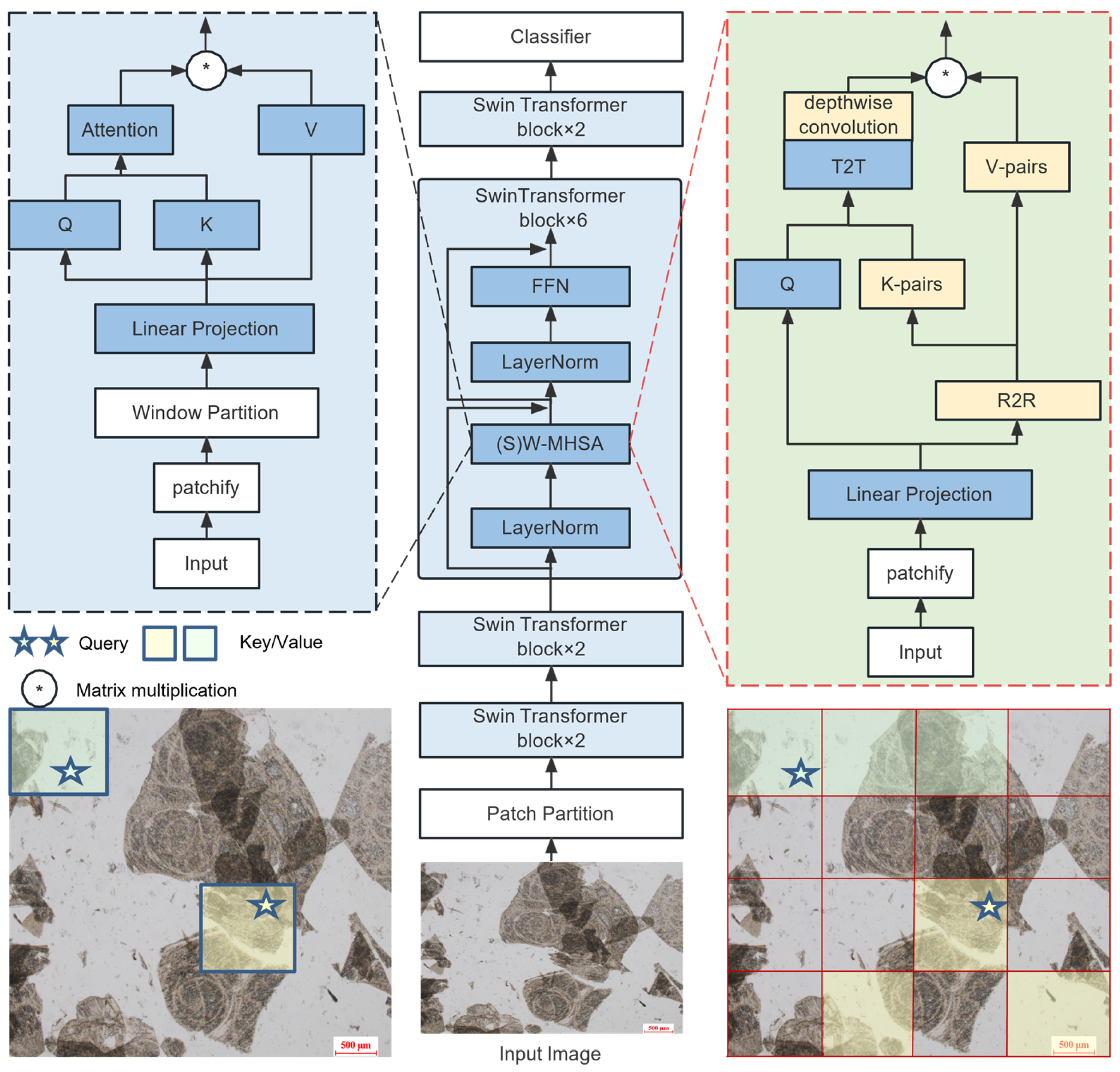
Firstly, we addressed the limitation of the Swin Transformer’s attention operation within a single local window by implementing a region-to-region approach [40]. Specifically, we first executed a region segmentation operation, partitioning the input image X (with a height of H, a width of W, and a channel number of C) into smaller blocks of size H/S. We assumed H to be equal to W, and S was set to the square root of the number of regions post-segmentation. The tensor representation is achieved by dividing the space into S × S distinct regions, each subjected to reshaping operations. This sequential aggregation forms a new tensor. The ensuing tensor’s dimensions are denoted as (S × S) × (H/S) × (W/S) × C. For simplification, we can express (S × S) × (H/S) × (W/S) as S2 × (H/S) × (W/S) × C. Further, (H/S) × (W/S) × C may be considered as a new dimension, reformulated as HW/S2 × C. Thus, our resulting tensor shape is S2 × HW/S2 × C. Here, S2 corresponds to the number of regions, HW/S2 quantifies the feature vectors within each region, and C indicates each feature vector’s channel count. A linear projection on X then generates the query, key, and value information.
Q = Xr Wq,
K = Xr Wk,
V = Xr Wv,
where Wq, Wk, Wv ∈ RC×C are the respective projection weights of the query, key, and value.
Subsequently, we determined the most relevant regions that require attention for each given area. By conducting average pooling on Q and K, we computed region-level queries and keys, denoted as Qr and Kr. The region adjacency matrix Ar was calculated by multiplying Qr with the transpose of Kr.
Ar = Qr (Kr)T.
Following this, we computed the index matrix Ir of the essential routing regions. This process involved pruning the affinity graph by retaining only the top k connections for each region.
Ir = topkIndex(Ar).
Thus, the ith row of Ir contains the k indices of the most relevant regions for the ith region.
After obtaining the index matrix Ir of the routing regions, we carried out a token-to-token attention operation on these regions [41]. For each query token in region i, we gathered all key-value pairs located in the union of k routing regions indexed by Ir.
Kg = gather (K,Ir),Vg = gather (V,Ir).
Having obtained this information, we applied the T2T attention and further enhanced it locally through deep convolution processing. This process allowed us to collect global context information within each region, which we then reassembled into a complete feature map, ready for input into the next block. The model’s overall framework adheres to the structure of the Swin Transformer-tiny, incorporating four stages with a block ratio of 2:2:6:2. We replaced the original window multi-head self-attention (W-MHSA) module in the block with our proposed method. The detailed network structure is depicted in Figure 2.

2.3. Experimental Setup and Evaluation Criteria

The experimental procedure is illustrated in the accompanying Figure 3. We selected three advanced models for our control experiment: ResNet 152 [42], ViT, and Swin Transformer. These models were trained using transfer learning to expedite model convergence. The experiment was implemented within the PyTorch framework, employing an NVIDIA RTXA4000 GPU with 17 GB of memory, was manufactured by NVIDIA and sourced from Huainan, China. We adjusted the input image size to 224 × 224 pixels. The cross-entropy loss function [43] was chosen as the rectifying function for backpropagation, and we set the batch size to 32. We trained our model using the AdamW [44] optimizer (β1 = 0.9, β2 = 0.999) and applied a learning rate scheduling strategy based on ReduceLROnPlateau (with mode = max, factor = 0.5 and patience = 10). We evaluated model performance using accuracy, precision, recall, and F1-scores as criteria.
Precision = TP/(TP + FP),
Recall = TP/(TP + FN),
F1-scores = 2 × (Precision × Recall)/(Precison + Recall).
Here, in the N × N confusion matrix, we call those judged as positive samples and are positive samples as true positive (TP); those judged as positive samples but are negative samples as false positive (FP); those judged as negative samples but are positive samples as false negative (FN); those judged as negative samples and are negative samples as true negative (TN).

3. Results

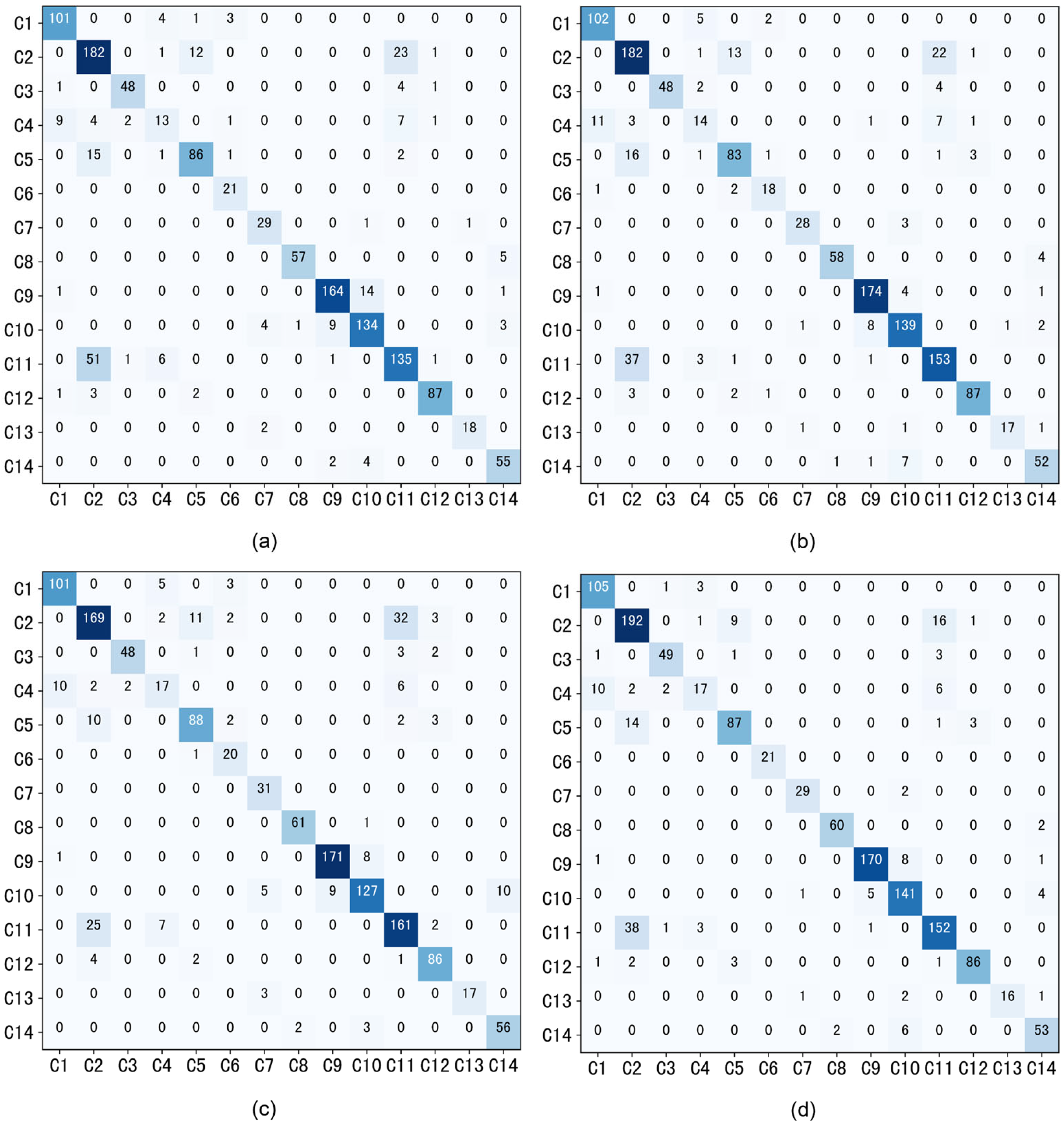
Table 2 lists the comparison results of the average Top-1 accuracy on Dataset 1. Our method achieves a Top-1 accuracy of 87.07% on the macro average and 88.04% on the weighted average. Moreover, as shown in Figure 4, according to the confusion matrix of different models, our method has the highest recognition accuracy in multiple categories, especially in the C2 category Debris Quartz Sandstone, where the accuracy reaches 87.67%.
We further conducted a detailed performance analysis of recall, precision, and F1-scores. The experimental comparison provided in Table 3 shows that our model has the highest recall, precision, and F1-scores in both the macro average and weighted average. Compared with the original Swin Transformer, it improves the F1-scores of all categories except for C3, C10, and C12.

4. Discussion

4.1. Explainable Analysis with SHAP

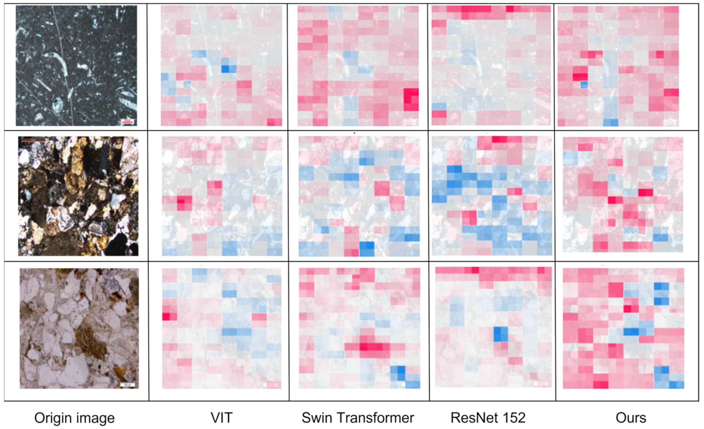
The interpretability of machine learning is relatively weak compared to traditional generalized linear models. Even though some models can train the importance of features, the scale standards of feature roles are inconsistent and lack intuitiveness; hence, they are often referred to as “black boxes”. This study uses the SHapley Additive exPlanation (SHAP) method to interpret the model [45,46]. SHAP analysis is a method of post hoc model interpretation and can interpret the output of any machine learning model. Based on the training status of tree models or neural networks, this method unifies the scale of feature importance for each sample and reflects the importance of features through SHAP values while also presenting the specific roles of each feature in each sample. We apply the SHAP method to the interpretive analysis of three types of rock thin-section images. By calculating the contribution of each pixel to the model’s predictive results, we visualize the decision-making process of the model in judging the rock. As shown in Figure 5, red pixels indicate a positive correlation, meaning the larger and darker the red area, the more favorable the model’s judgment of the rock. Conversely, the larger and darker the blue pixel area, the more unfavorable it is for the model’s judgment. The results show that our method can more accurately locate and interpret the key features in the rock compared to the other three advanced models.

4.2. Model Complexity Analysis

We compared the average running time on Dataset 1, where the resolution of the input images is 224 × 224. Table 4 lists the average running time, the number of parameters, GFLOPs, and model size of the three most advanced models and our model. Please note that all times are measured on the same computing platform with a single RTXA4000 GPU. Although the number of parameters and GFLOPs of our model is slightly increased compared to the Swin Transformer, the average running speed is faster. Compared to the other two models, our model not only performs optimally but also significantly reduces the number of parameters, greatly reducing the need for storage and computational resources.

4.3. Generalization Analysis

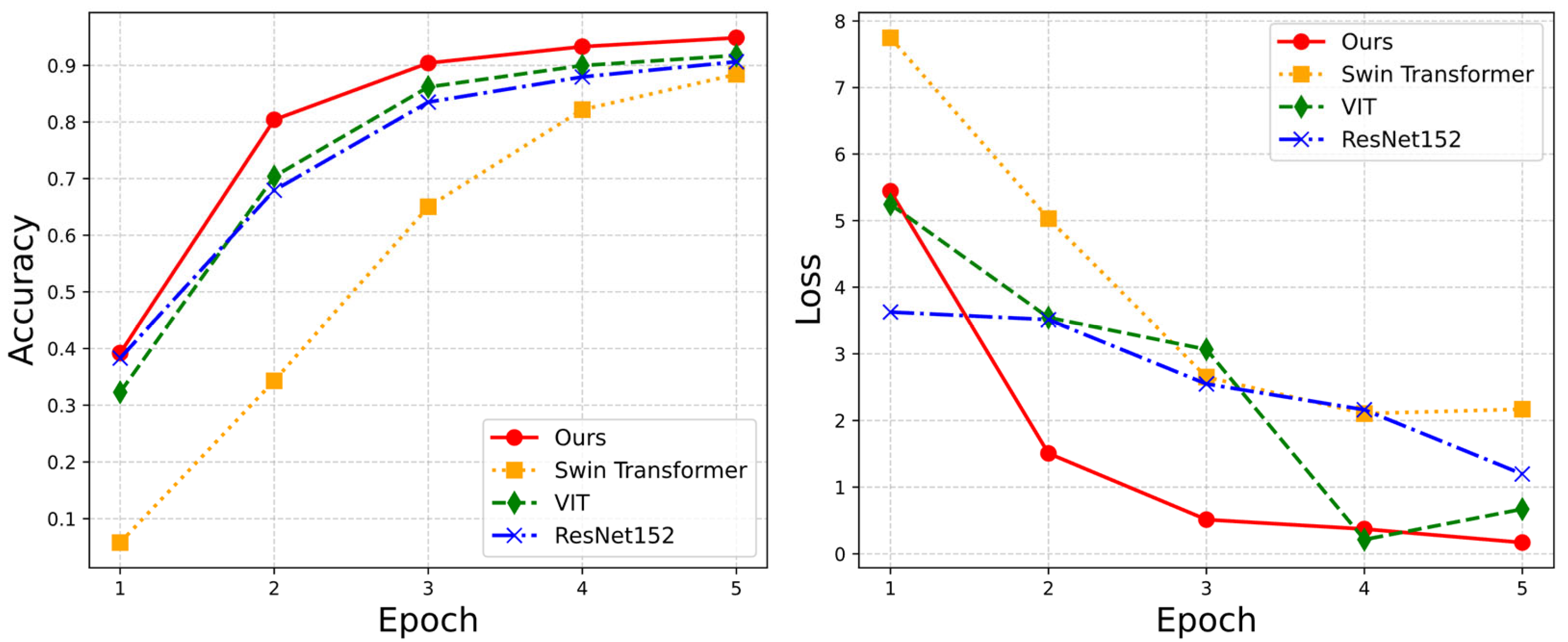
To verify the generalization ability and robustness of our model, the model trained on Dataset 1 was tested on Dataset 2. Figure 6 compares the generalization performance of our model with the three most advanced models. After five rounds, in terms of generalization capability analysis, our method shows significant advantages. Our model still shows the highest Top-1 accuracy, performing best among all models. Additionally, according to the loss curve, our model has better stability.

4.4. Limitations

Transformer models use self-attention mechanisms, thereby performing well in capturing long-range dependencies in input data and understanding global structures and local features in images. Our model has mitigated the problem of sample scarcity in Transformers. However, compared to CNN models, Transformer models still need more training samples to extract rich features [47], and the amount of publicly available thin rock section data is far from sufficient. Furthermore, the incorporation of a nominal quantity of disparate rock samples aimed at diversifying the dataset could induce a long-tail distribution [48]. This might precipitate an unfair outcome in comparative analysis. Consequently, we deliberately omitted igneous rocks from our current investigation. On the other hand, the significant differences between samples in the source domain and target domain limited the effectiveness of transfer learning techniques in this experiment. Therefore, the performance of the Vision Transformer and Swin Transformer is still not as good as that of ResNet-152. The recognition result of Feldspar Debris Sandstone performed the worst. It can be clearly seen that due to the lack of training samples, it is difficult for the model to distinguish it from the extremely similar Debris Feldspar Sandstone.

5. Conclusions

In this research, we enhanced the Swin Transformer’s performance in ultra-fine grain classification of sandstone and limestone by integrating the region-to-region (R2R) method and token-to-token (T2T) attention mechanisms. The novelty of our approach lies in its capacity to extend beyond the constraint of an independent local window for attention operation, incorporating the most relevant adjacent regions for computation. This strategy significantly enriches the capture density of global information. We then executed token-to-token attention operations along with deep convolution operations within these related regions to capture fine-grained details more effectively. When compared with three other advanced models, our model consistently outperformed in all four measures—accuracy, precision, recall, and F1-score—both in macro and weighted averages. The interpretive analysis based on SHAP reveals that our model can more accurately locate and interpret key features in thin-section images. Simultaneously, the model has significant advantages in complexity, with a low number of parameters and computational complexity, and can provide excellent performance. This makes our method more feasible and sustainable in practical applications. Furthermore, our model demonstrated robustness in generalization analysis, signifying its potential as a reference for subsequent ultra-fine grain recognition tasks across different rock categories. Certainly, experimental research possesses numerous avenues for further exploration. One critical issue meriting future investigation is the incorporation of a broader range of rock samples into the experiments without compromising the fairness of results. Future research might focus on several areas. First, in the context of an expanded array of rock samples, there is a need to investigate strategies for enhancing the performance of the Visual Transformer model and for addressing the long-tail distribution issue in rock classification tasks. Second, it is crucial to identify methods that bridge the performance disparity between the Visual Transformer model and the CNN model on small datasets. Simultaneously, research should concentrate on how to harness the full potential of the Transformer model when the sample size is limited.

Author Contributions

Conceptualization, project administration, visualization, H.Z. and S.W.; methodology, software, investigation, data curation, writing—original draft preparation, formal analysis, validation, S.W.; supervision, writing—review and editing, H.Z. All authors have read and agreed to the published version of the manuscript.

Funding

This research was supported by Coal Industry Engineering Research Center for Comprehensive Prevention and Control of Mine Water Disaster (2022-CIERC-03). Research on rock recognition of intelligent terminal (2022CX2008) was conducted in association with the Graduate Innovation Fund Project of Anhui University of Science and Technology. Funding was also received from the Scientific Research Foundation for High-level Talents of Anhui University of Science and Technology.

Institutional Review Board Statement

Not applicable.

Informed Consent Statement

Not applicable.

Data Availability Statement

The data in this study are available from the corresponding authors upon request.

Conflicts of Interest

The authors declare no conflict of interest.

References

  1. Xu, Z.; Ma, W.; Lin, P.; Hua, Y. Deep Learning of Rock Microscopic Images for Intelligent Lithology Identification: Neural Network Comparison and Selection. J. Rock Mech. Geotech. Eng. 2022, 14, 1140–1152. [Google Scholar] [CrossRef]
  2. Liu, N.; Huang, T.; Gao, J.; Xu, Z.; Wang, D.; Li, F. Quantum-Enhanced Deep Learning-Based Lithology Interpretation from Well Logs. IEEE Trans. Geosci. Remote Sens. 2021, 60, 4503213. [Google Scholar] [CrossRef]
  3. Pi, Z.; Zhou, Z.; Li, X.; Wang, S. Digital Image Processing Method for Characterization of Fractures, Fragments, and Particles of Soil/Rock-like Materials. Mathematics 2021, 9, 815. [Google Scholar] [CrossRef]
  4. Martínez-Martínez, J.; Corbí, H.; Martin-Rojas, I.; Baeza-Carratalá, J.F.; Giannetti, A. Stratigraphy, Petrophysical Characterization and 3D Geological Modelling of the Historical Quarry of Nueva Tabarca Island (Western Mediterranean): Implications on Heritage Conservation. Eng. Geol. 2017, 231, 88–99. [Google Scholar] [CrossRef] [Green Version]
  5. Izadi, H.; Sadri, J.; Bayati, M. An Intelligent System for Mineral Identification in Thin Sections Based on a Cascade Approach. Comput. Geosci. 2017, 99, 37–49. [Google Scholar] [CrossRef]
  6. Vaneghi, R.G.; Saberhosseini, S.E.; Dyskin, A.V.; Thoeni, K.; Sharifzadeh, M.; Sarmadivaleh, M. Sources of Variability in Laboratory Rock Test Results. J. Rock Mech. Geotech. Eng. 2021, 13, 985–1001. [Google Scholar] [CrossRef]
  7. Thompson, S.; Fueten, F.; Bockus, D. Mineral Identification Using Artificial Neural Networks and the Rotating Polarizer Stage. Comput. Geosci. 2001, 27, 1081–1089. [Google Scholar] [CrossRef]
  8. Singh, N.; Singh, T.; Tiwary, A.; Sarkar, K.M. Textural Identification of Basaltic Rock Mass Using Image Processing and Neural Network. Comput. Geosci. 2010, 14, 301–310. [Google Scholar] [CrossRef]
  9. Chatterjee, S. Vision-Based Rock-Type Classification of Limestone Using Multi-Class Support Vector Machine. Appl. Intell. 2013, 39, 14–27. [Google Scholar] [CrossRef]
  10. Zhang, Y.; Li, M.; Han, S.; Ren, Q.; Shi, J. Intelligent Identification for Rock-Mineral Microscopic Images Using Ensemble Machine Learning Algorithms. Sensors 2019, 19, 3914. [Google Scholar] [CrossRef] [Green Version]
  11. Polat, Ö.; Polat, A.; Ekici, T. Automatic Classification of Volcanic Rocks from Thin Section Images Using Transfer Learning Networks. Neural Comput. Appl. 2021, 33, 11531–11540. [Google Scholar] [CrossRef]
  12. Alzubaidi, F.; Mostaghimi, P.; Swietojanski, P.; Clark, S.R.; Armstrong, R.T. Automated Lithology Classification from Drill Core Images Using Convolutional Neural Networks. J. Pet. Sci. Eng. 2021, 197, 107933. [Google Scholar] [CrossRef]
  13. Ma, H.; Han, G.; Peng, L.; Zhu, L.; Shu, J. Rock Thin Sections Identification Based on Improved Squeeze-and-Excitation Networks Model. Comput. Geosci. 2021, 152, 104780. [Google Scholar] [CrossRef]
  14. Li, D.; Zhao, J.; Ma, J. Experimental Studies on Rock Thin-Section Image Classification by Deep Learning-Based Approaches. Mathematics 2022, 10, 2317. [Google Scholar] [CrossRef]
  15. De Lima, R.P.; Duarte, D.; Nicholson, C.; Slatt, R.; Marfurt, K.J. Petrographic Microfacies Classification with Deep Convolutional Neural Networks. Comput. Geosci. 2020, 142, 104481. [Google Scholar] [CrossRef]
  16. YU, X. Ultra-Fine-Grained Visual Categorization. PhD Thesis, Griffith University, Australia, 2021. [Google Scholar]
  17. Liang, Y.; Cui, Q.; Luo, X.; Xie, Z. Research on Classification of Fine-Grained Rock Images Based on Deep Learning. Comput. Intell. Neurosci. 2021, 2021, 5779740. [Google Scholar] [CrossRef]
  18. Yu, X.; Wang, J.; Zhao, Y.; Gao, Y. Mix-ViT: Mixing Attentive Vision Transformer for Ultra-Fine-Grained Visual Categorization. Pattern Recognition 2023, 135, 109131. [Google Scholar] [CrossRef]
  19. Vaswani, A.; Shazeer, N.; Parmar, N.; Uszkoreit, J.; Jones, L.; Gomez, A.N.; Kaiser, L.; Polosukhin, I. Attention Is All You Need. arXiv 2017, arXiv:1706.03762. [Google Scholar]
  20. Dosovitskiy, A.; Beyer, L.; Kolesnikov, A.; Weissenborn, D.; Zhai, X.; Unterthiner, T.; Dehghani, M.; Minderer, M.; Heigold, G.; Gelly, S.; et al. An Image Is Worth 16 × 16 Words: Transformers for Image Recognition at Scale. arXiv 2020, arXiv:2010.11929. [Google Scholar]
  21. Liu, Z.; Lin, Y.; Cao, Y.; Hu, H.; Wei, Y.; Zhang, Z.; Lin, S.; Guo, B. Swin Transformer: Hierarchical Vision Transformer Using Shifted Windows. In Proceedings of the IEEE/CVF International Conference on Computer Vision, Montreal, BC, Canada, 11–17 October 2021; pp. 10012–10022. [Google Scholar]
  22. Zheng, Y.; Jiao, L.; Wu, W.; Zhang, C. Petrographic Recognition and Classification of Bioclastic Carbonate Thin Sections Based on Attention Mechanism. Geoenergy Sci. Eng. 2023, 225, 211712. [Google Scholar] [CrossRef]
  23. Huang, Z.; Su, L.; Wu, J.; Chen, Y. Rock Image Classification Based on EfficientNet and Triplet Attention Mechanism. Appl. Sci. 2023, 13, 3180. [Google Scholar] [CrossRef]
  24. Xu, Y.; Hu, X.; Sun, G.; A Photomicrograph Dataset of Mid-Cretaceous Langshan Formation from the Northern Lhasa Terrane, Tibet. Science Data Bank. Available online: https://www.scidb.cn/en/detail?dataSetId=724638692169220096 (accessed on 10 May 2022).
  25. Han, Z.; Hu, X.; A Photomicrograph Dataset of the Early-Middle Jurassic Rocks under Thin Section in the Tibetan Tethys Himalaya. Science Data Bank. Available online: https://www.scidb.cn/en/detail?dataSetId=722014393801375744 (accessed on 10 May 2022).
  26. Hu, X.; Data Set of Polarizing Micrographs of Late Cretaceous-Eocene Rock Slices in the Western Tarim Basin, Xinjiang. Science Data Bank. Available online: https://www.scidb.cn/en/detail?dataSetId=683352400798416896 (accessed on 10 May 2022).
  27. Zhang, Y.; An, W.; Hu, X.; A Photomicrograph Dataset of Cretaceous Siliciclastic Rocks from Xigaze Forearc Basin, Southern Tibet. Science Data Bank. Available online: https://www.scidb.cn/en/detail?dataSetId=731595076429414400 (accessed on 10 May 2022).
  28. Lai, W.; Zhang, Y.; Hu, X.; Sun, G.; Photomicrograph Dataset of Cretaceous Siliciclastic Rocks from the Central-Northern Lhasa Terrane. Tibet Science Data Bank. Available online: https://www.scidb.cn/en/detail?dataSetId=684034823831945216 (accessed on 10 May 2022).
  29. Liu, Y.; Hou, M.; Liu, X.; Qi, Z.; A Micrograph Dataset of Buried Hills and Overlying Glutenite in Bozhong Sag, Bohai Bay Basin. Science Data Bank. Available online: https://www.scidb.cn/en/detail?dataSetId=752623639467130880 (accessed on 10 May 2022).
  30. Du, X.; Microscopic Image Data Set of Xujiahe Gas Reservoir in Northeast Sichuan. Science Data Bank. Available online: https://www.scidb.cn/en/detail?dataSetId=b068f97abd9b4b6da1558bcc20337632 (accessed on 10 May 2022).
  31. Shi, G.; Hu, Z.; Li, Y.; Liu, C.; Guan, J.; Chen, H.; Hou, M.; Wang, F.; A Sandstone Microscopical Images Dataset of He-8 Member of Upper Paleozoic in Northeast Ordos Basin. Science Data Bank. Available online: https://www.scidb.cn/en/detail?dataSetId=727528044247384064 (accessed on 10 May 2022).
  32. Li, P.; Li, Y.; Cheng, X.; Wang, Y.; Li, C.; Liu, Z.; A Photomicrograph Dataset of Upper Paleozoic Tight Sandstone from Linxing Block, Eastern Margin of Ordos Basin. Science Data Bank. Available online: https://www.scidb.cn/en/detail?dataSetId=727601552654598144 (accessed on 10 May 2022).
  33. Cai, W.; Hou, M.; Chen, H.; Liu, Y.; A Micrograph Dataset of Terrigenous Clastic Rocks of Upper Devonian Lower Carboniferous Wutong Group in Southern Lower Yangtze. Science Data Bank. Available online: https://www.scidb.cn/en/detail?dataSetId=732987889075355648 (accessed on 10 May 2022).
  34. Feng, W.; He, F.; Zhou, Y.; Yang, J.; A Microscopic Image Dataset of Permian Volcanolithic Fragment Bearing Sandstones from SouthWest China. Science Data Bank. Available online: https://www.scidb.cn/en/detail?dataSetId=703351065692602368 (accessed on 10 May 2022).
  35. Ma, Q.; Chai, R.; Yang, J.; Du, Y.; Dai, X.; A Microscopic Image Dataset of Mesozoic Metamorphic Grains Bearing Sandstones from Mid-Yangtze, China. Science Data Bank. Available online: https://www.scidb.cn/en/detail?dataSetId=727525043063488512 (accessed on 10 May 2022).
  36. Dunham, R.J. Classification of sedimentary rocks according to depositional texture. In Classification of Carbonate Rocks, Memoir 1, American; Ham, W.E., Ed.; Association of Petroleum Geologists: Tulsa, OK, USA, 1962; pp. 108–121. [Google Scholar]
  37. Embry, A.F.; Klovan, J.E. A Late Devonian Reef Tract on Northeastern Banks Island, NWT. Bull. Can. Pet. Geol. 1971, 19, 730–781. [Google Scholar]
  38. Garzanti, E. From Static to Dynamic Provenance Analysis—Sedimentary Petrology Upgraded. Sediment. Geol. 2016, 336, 3–13. [Google Scholar] [CrossRef]
  39. Lai, W.; Jiang, J.; Qiu, J.; Yu, J.; Hu, X.; A Photomicrograph Dataset of Rocks for Petrology Teaching at Nanjing University. Science Data Bank. Available online: https://www.scidb.cn/en/detail?dataSetId=732953783604084736 (accessed on 10 May 2022).
  40. Zhu, L.; Wang, X.; Ke, Z.; Zhang, W.; Lau, R.W. BiFormer: Vision Transformer with Bi-Level Routing Attention. In Proceedings of the IEEE/CVF Conference on Computer Vision and Pattern Recognition, Vancouver, BC, Canada, 18–22 June 2023; pp. 10323–10333. [Google Scholar]
  41. Yuan, L.; Chen, Y.; Wang, T.; Yu, W.; Shi, Y.; Jiang, Z.-H.; Tay, F.E.; Feng, J.; Yan, S. Tokens-to-Token Vit: Training Vision Transformers from Scratch on Imagenet. In Proceedings of the IEEE/CVF International Conference on Computer Vision, Montreal, BC, Canada, 11–17 October 2021; pp. 558–567. [Google Scholar]
  42. He, K.; Zhang, X.; Ren, S.; Sun, J. Deep Residual Learning for Image Recognition. In Proceedings of the IEEE Conference on Computer Vision and Pattern Recognition, Las Vegas, NV, USA, 27–30 June 2016; pp. 770–778. [Google Scholar]
  43. Szegedy, C.; Vanhoucke, V.; Ioffe, S.; Shlens, J.; Wojna, Z. Rethinking the Inception Architecture for Computer Vision. In Proceedings of the IEEE Conference on Computer Vision and Pattern Recognition, Las Vegas, NV, USA, 27–30 June 2016; pp. 2818–2826. [Google Scholar]
  44. Loshchilov, I.; Hutter, F. Decoupled Weight Decay Regularization. arXiv 2017, arXiv:1711.05101. [Google Scholar]
  45. Nohara, Y.; Matsumoto, K.; Soejima, H.; Nakashima, N. Explanation of Machine Learning Models Using Shapley Additive Explanation and Application for Real Data in Hospital. Comput. Methods Programs Biomed. 2022, 214, 106584. [Google Scholar] [CrossRef]
  46. Rodríguez-Pérez, R.; Bajorath, J. Interpretation of Compound Activity Predictions from Complex Machine Learning Models Using Local Approximations and Shapley Values. J. Med. Chem. 2019, 63, 8761–8777. [Google Scholar] [CrossRef]
  47. Steiner, A.; Kolesnikov, A.; Zhai, X.; Wightman, R.; Uszkoreit, J.; Beyer, L. How to Train Your Vit? Data, Augmentation, and Regularization in Vision Transformers. arXiv 2021, arXiv:2106.10270. [Google Scholar]
  48. Xu, Z.; Liu, R.; Yang, S.; Chai, Z.; Yuan, C. Learning Imbalanced Data with Vision Transformers. In Proceedings of the IEEE/CVF Conference on Computer Vision and Pattern Recognition, Vancouver, BC, Canada, 18–22 June 2023; pp. 15793–15803. [Google Scholar]
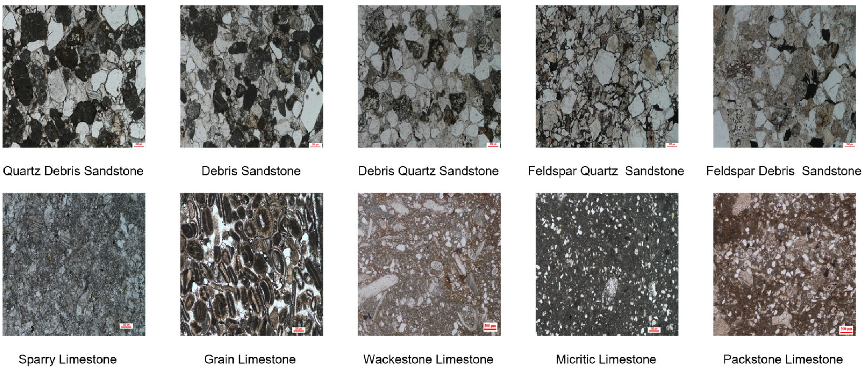
Figure 1. The ultra-fine-grained categories of 10 types of rocks. Due to the slight visual differences between thin sections of rocks from different categories, it is very challenging to distinguish the ultra-fine-grained categories of these 10 types of rocks. For example, the visual differences between quartz debris sandstone and debris sandstone, as well as debris quartz sandstone, are very subtle.
Applsci 13 07853 g001
Figure 2. Improved network structure diagram. The diagram on the left represents the attention module used in each block of the original model, where the operation of each node is confined to a single local window. The one on the right is an improved module where each node can perform attention operations within multiple related windows.
Applsci 13 07853 g002
Figure 3. Flowchart of the training and evaluation process for each model in this study.
Applsci 13 07853 g003
Figure 4. Confusion matrices of four models, where (a) is ViT, (b) is Swin Transformer, (c) is ResNet152, and (d) is our improved model. C1–C14 are named according to the order of rocks in dataset1 in Table 1.
Applsci 13 07853 g004
Figure 5. SHAP interpretability analysis diagrams of the four models for rocks. color intensity represents the strength of correlation; darker shades of red indicate stronger positive correlations, while darker shades of blue denote stronger negative correlations.
Applsci 13 07853 g005
Figure 6. Accuracy and loss curves of the four models tested on Dataset 2.
Applsci 13 07853 g006
Table 1. Dataset statistics.
DatasetIDClassNumbers
Subclass
Number
TrainTest
Dataset1C1Debris Feldspar Sandstone111,3531360
C2Debris Quartz Sandstone1
C3Debris Sandstone1
C4Feldspar Debris Sandstone1
C5Feldspar Quartz Sandstone1
C6Feldspar Sandstone1
C7Quartz Debris Sandstone1
C8Quartz Sandstone1
C9Floatstone limestone1
C10Grain Limestone1
C11Micritic Limestone1
C12Packstone Limestone1
C13Quartz Debris Sandstone1
C14Quartz Sandstone1
Dataset2 Metamorphic Rock402185449
Sedimentary Rock28
Volcanic Rock40
Table 2. The average Top-1 accuracy on Dataset 1.
ResNet152ViTSwin TransformerOurs
macro avg86.65%85.00%84.50%87.07%
weighted avg86.17%84.45%86.32%88.04%
Table 3. Results of recall, precision, and F1-scores on Dataset 1.
Categories Metrics (%)Models
ResNet-152ViTSwin TransformerOurs
C1Precision0.90180.89380.88700.8898
Recall0.92660.92660.93580.9633
F1-score0.91400.90990.91070.9251
C2Precision0.80480.71370.75520.7742
Recall0.77170.83110.83110.8767
F1-score0.78790.76790.79130.8223
C3Precision0.96000.94121.00000.9245
Recall0.88890.88890.88890.9074
F1-score0.92310.91430.94120.9159
C4Precision0.54840.52000.53850.7083
Recall0.45950.35140.37840.4595
F1-score0.50000.41940.44440.5574
C5Precision0.85440.85150.82180.8700
Recall0.83810.81900.79050.8286
F1-score0.84620.83500.80580.8488
C6Precision0.74070.80770.81821.0000
Recall0.95241.00000.85711.0000
F1-score0.83330.89360.83721.0000
C7Precision0.79490.82860.93330.9355
Recall1.00000.93550.90320.9355
F1-score0.88570.87880.91800.9355
C8Precision0.96830.98280.98310.9677
Recall0.98390.91940.93550.9677
F1-score0.97600.95000.95870.9677
C9Precision0.95000.93180.94050.9659
Recall0.95000.91110.96670.9444
F1-score0.95000.92130.95340.9551
C10Precision0.91370.87580.90260.8868
Recall0.84110.88740.92050.9338
F1-score0.87590.88160.91150.9097
C11Precision0.78540.78950.81820.8492
Recall0.82560.69230.78460.7795
F1-score0.80500.73770.80100.8128
C12Precision0.89580.95600.94570.9556
Recall0.92470.93550.93550.9247
F1-score0.91010.94570.94050.9399
C13Precision1.00000.94740.94441.0000
Recall0.85000.90000.85000.8000
F1-score0.91890.92310.89470.8889
C14Precision0.84850.85940.86670.8689
Recall0.91800.90160.85250.8689
F1-score0.88190.88000.85950.8689
macro avgPrecision0.85480.84990.86820.8997
Recall0.86650.85000.84500.8707
F1-score0.85770.84700.85490.8820
weighted avgPrecision0.86230.84530.86260.8813
Recall0.86170.84450.86320.8804
F1-score0.86090.84280.86190.8790
Table 4. Detailed parameters of the four models.
ModelsAverage Runtime (MS)Params(M)GFLOPsInput SizeModel Size
ResNet15252.3458.223.20224 × 224222.8
ViT14.8458.122.57224 × 224330.3
Swin Transformer32.3919.65.96224 × 224108.2
Ours23.5321.96.70224 × 224108.3
Disclaimer/Publisher’s Note: The statements, opinions and data contained in all publications are solely those of the individual author(s) and contributor(s) and not of MDPI and/or the editor(s). MDPI and/or the editor(s) disclaim responsibility for any injury to people or property resulting from any ideas, methods, instructions or products referred to in the content.