1. Introduction
Reliable prediction of structural responses is essential in analyzing, designing, and evaluating buildings under earthquake effects. In recent years, substantial research has been devoted to developing efficient, rapid, and reliable methods for estimating these responses using approximate solutions. Among the approximate methods, continuous beam models have become preferred for dynamic analysis, preliminary design, and assessment of buildings under earthquake effects [
1,
2,
3,
4,
5,
6,
7,
8,
9,
10,
11,
12,
13]. Buildings are classified according to specific height ranges in the codes: generally, low-rise up to four or five stories, high-rise after 12 stories, and mid-rise buildings in between. As the number of stories increases, these approximate models are preferred for modeling mid- and high-rise buildings, generally named multistory buildings [
14]. These studies have explored the influence of mass and stiffness distributions, both uniform and nonuniform, along the height of buildings on their structural behavior. Heidebrecht and Rutenberg [
15] presented an alternative formulation for assessing the upper and lower bounds of inter-story drift demands in frame structures, which diverged from the original method proposed by Heidebrecht and Stafford Smith [
1]. Miranda [
4] refined the idea of the coupling beam. Notably, Miranda and Reyes [
16] extended the work of Miranda [
4] to address nonuniform stiffness distributions and demonstrated that, unless there are abrupt and significant stiffness changes, they do not significantly impact the structural behavior.
Similarly, Miranda and Taghavi [
5] and Taghavi and Miranda [
6,
17] investigated floor acceleration demands using a continuous shear–flexural beam model with nonuniform stiffness for low and medium-height buildings. Reinoso and Miranda [
18] focused on acceleration demands in tall buildings. Miranda and Akkar [
6] derived the generalized inter-story drift spectrum for buildings under earthquake ground motions. Alonso-Rodríguez and Miranda [
10] analyzed the continuous shear–flexural beam model with a shear beam featuring a parabolic variable stiffness and a Bernoulli beam with fourth-order flexural stiffness. In a recent study, Alonso-Rodríguez and Tsavdaridis [
12] investigated the effects of rotational inertia on the structural behavior of the continuous shear–flexural beam model. Lai et al. [
19] employed a continuous shear–flexural beam model with nonuniform mass and stiffness distributions along the height to estimate the elastic inter-story drift demands in super high-rise buildings. In addition to developing the continuous shear–flexural beam model by considering mass and stiffness variations, there have been studies on the capabilities of and their applications in structural response prediction of this approximate model in recent years. Huergo and Hernández [
20,
21] investigated tall buildings’ dynamic analysis and soil–structure interaction with tuned mass dampers (TMDs) using the continuous shear–flexural beam model. Guo et al. [
22] investigated the self-similar inter-story drift and response distribution using a shear–flexural beam model with nonuniform lateral stiffness. Ghahari et al. [
23] presented a method for quantifying modeling uncertainty in approximate methods used in building response prediction and applied it to a coupled shear–flexural beam model. Ranaiefar et al. [
24] estimated the seismic inter-story drift in tall buildings by applying mode acceleration instead of mode displacement to a shear–flexural beam model.
Lateral displacements and inter-story drift demands are the main cause of structural damage in buildings when subjected to lateral loads. In many studies, the inter-story drift ratio has been denoted as the most critical parameter associated with damage occurring in buildings under lateral forces [
6,
25,
26,
27,
28,
29,
30], and limitations on the inter-story drift ratio have been introduced in the building codes [
31,
32].
The drift ratios along the height of a building do not exhibit a uniform distribution, and they attain their maximum values at specific stories according to the structural behavior. Since the maximum inter-story drift ratio is directly associated with structural damage, it is also essential to determine the location within the building this maximum response occurs [
7]. Khaloo and Khosravi [
7] conducted a comprehensive investigation of the behavior of structures under pulse-type ground motions in near-field earthquakes using a continuous beam model. They analyzed the maximum displacement spectrum, maximum inter-story drift ratio spectrum, and maximum inter-story drift height spectrum. Similarly, Neam and Taghikhang [
26] and Eroglu [
27] proposed a logarithmic function based on seismic and geotechnical information to estimate the maximum inter-story drift. This function was employed in probabilistic seismic analysis and design methods.
Previous studies [
1,
3,
4,
5,
8] have typically assumed the base point’s boundary condition of zero when solving the differential equations for continuous beam models. However, this approach does not accurately reflect the first story drift, as the rotation in the displacement function of the continuous model provides the inter-story drift ratio [
6,
7,
12]. In the study by Eroǧlu and Akkar [
33], a new lateral stiffness coefficient that is story-dependent along the building height was proposed for frame-type buildings, considering the model by Heidebrecht and Stafford Smith [
1].
In this study, the dynamic response of a shear–flexural continuous beam model is elucidated by solving the equation of motion, wherein the rotation (θ) is introduced at the base. The closed-form solutions are obtained, and the lateral displacement and inter-story drift demands are investigated. Closed-form solutions of the displacement and inter-story drift equations are obtained depending on the lateral stiffness ratio (α) and the initial rotation (θ). The lateral stiffness ratio (α) plays a crucial role in determining the structural behavior on the basis of the stiffness of elements within the building systems, emphasizing the significance of its accurate definition. To this end, a simple function for the lateral stiffness ratio based on the beam–column stiffness ratio and the number of stories is proposed. The function coefficients are determined through fitting analysis using data obtained from finite element analysis. In order to demonstrate the accuracy of the proposed method, the results obtained by analyzing different building type structures with the finite element program sap2000 and the results obtained with the proposed method are compared.
In conclusion, the proposed study presents a novel closed-form solution for the continuous beam model, incorporating a rotation (θ) at the base. The model’s effectiveness in predicting building behavior could be validated through comprehensive dynamic analyses and comparative results. The accurate estimation of critical parameters and their applicability to low-rise buildings position the model as a noteworthy advancement in structural engineering.
2. Continuous Shear–Flexural Beam Model
Despite the complex analysis of multi-degree-of-freedom (discrete mass) systems, continuous models are widely used in the literature as approximate methods. In recent years, various continuous beam models and simplified versions based on beam theories have been proposed to predict structural responses. Typically, these simplified models consider a continuous cantilever beam with uniform mass and stiffness distributions along its height. In these studies, displacement and rotation are taken to be zero as the base boundary condition. This approach does not fully represent the behavior of the structure since rotation gives drift in the continuous model. This study aims to enhance the continuous system model approach and improve predictions of structural responses by introducing a closed-form solution that incorporates a rotation (θ) boundary condition at the base, as utilized by Miranda and Taghavi [
5] in their continuous shear–flexural beam model with fixed base.
When subjected to a horizontal ground acceleration ü
g(t) at the base, the undamped motion equation of the continuous beam model is formulated as a partial derivative differential equation, represented as Equation (1).
where m is the mass per unit length, H is the total height of the building, u(ζ,t) is the lateral displacement at dimensionless height ζ = z/H at time t, EI is the flexural rigidity of the flexural beam, and the lateral stiffness ratio (α) is a dimensionless parameter that determines the extent of flexure and shear deformations in the continuous model, thereby controlling the lateral deformation along the height. For α = 0, the continuous model behaves as a Euler–Bernoulli beam, while α → ∞ corresponds to a pure shear beam. Intermediate values of α correspond to multistory buildings exhibiting combined flexure and shear deformations [
5].
where GA is the shear rigidity of the shear beam. Miranda [
4] specified the range of α as 0 to 30 for conventional structures and defined different ranges on the basis of the structural system type. Shear wall systems exhibit α values within 0 < α < 2, while dual systems (moment-resisting frame–wall or moment-resisting frame–cross braced systems) fall within 1.5 < α < 6. Moment-resisting frame systems typically have α values ranging from 5 to 20, while α values greater than 30 represent shear frame behavior. Taghavi and Miranda [
6,
16] used the average values of these ranges according to the type of structural system in their building models. They suggested that this value can be used as 3.125 for dual systems and 12.5 for moment-resisting frame systems. Since moment-resisting frame systems are analyzed in this study, Miranda’s α approximation is considered as 12.5.
For linear elastic structures, the responses can be obtained by combining the responses of all modes. The displacement expression (u(ζ,t)) at dimensionless height ζ and time t for a continuous structure can be calculated using a linear combination of modal responses.
Considering classical damping, the contribution of each mode to the response, in terms of lateral displacement (u
i(ζ,t)) and inter-story drift ratio (IDR
i(ζ,t)), is determined as follows:
Here, the modal participation factor (Γ
i) for the continuous model with uniform mass distribution is given by
By substituting Equation (4) into Equation (1) and solving for the free vibration case using the separation of variables method, two partial equations dependent on location (ϕ
i(ζ)) and time (D
i(t)) are obtained:
The general solution of Equation (8) provides the mode shape function (ϕ
i (ζ)):
where B
1–4 represents the integration constants obtained based on the boundary conditions.
The eigenvalue (γ
i) is derived from the solution of the circular frequencies (ω
i) using Equation (10).
In this case, the period ratios (T
i/T
1) for the continuous beam model are determined as follows:
The mode shape function (ϕ(ζ)), drift mode shape function (ϕʹ(ζ)), modal participation factor (Γ
i), and period ratios (T
i/T
1) solely depend on the lateral stiffness ratio α [
5,
6]. Accurate dynamic properties and structural response prediction can be achieved by selecting the appropriate value of α [
4]. In addition to these parameters, information regarding the structure’s fundamental vibration period and damping ratios is required for modal analysis. Miranda and Taghavi [
5] suggested using the period equations proposed by Heidebrecht and Smith [
1] or Rutenberg [
34] to calculate the fundamental vibration period of the continuous model.
Implementation of Boundary Conditions
When the continuous model is fixed at the base, the boundary conditions include displacement and rotation of zero at the base. However, in the proposed model, the displacement at the base is zero, while a rotation (θ) is defined, which differs from zero. The following equations can express this:
The case where the rotation is zero (θ = 0) provides the same solution as presented by Miranda and Taghavi [
5].
Similarly, in the continuous model, at the free end, the boundary condition at the normalized height (ζ = 1) results in zero moment and shear force:
The integration constants obtained using the boundary conditions are as follows:
The B
1-4 integration constants given in Equations (12)–(14) are used to substitute the mode shape function given in Equation (9) into the boundary condition Equation (15), resulting in the characteristic Equation (16).
By solving the characteristic Equation (Equation (16)), which is a function of α and θ, the eigenvalues (γi) of the equation are obtained.
The rotation (θ) at the base is defined as the displacement ratio of the ground story. In this case, the expression “θ” is defined as the ratio of the ground story height (h
1) to the building height (H) through the normalized height (ζ).
When considering the case where all stories have equal story heights (h1 = hj), the definition of θ is equal to “1/N”, where N is the number of stories. In this study, equal story heights are assumed for all stories.
The continuous model with a uniform mass and stiffness distribution along the height, mode shapes, period ratios, and modal participation factors depends on dimensionless base rotation and lateral stiffness ratio parameters. The base rotation is defined as the drift ratio of the first story. The remaining lateral stiffness ratio needs to be known. In the literature, approximate ranges for this coefficient have been determined on the basis of the structural system of the building, but no definitive calculation has been suggested. In the subsequent parts of the study, a simple empirical equation is proposed for the lateral stiffness ratio using a curve fitting method to provide more accurate predictions of structural responses.
3. Estimation of Lateral Stiffness Ratio
The displacement of buildings under horizontal loads is determined by the bending deformation of the columns and the rotation of the beams connected to the ends of the columns, which is influenced by their respective stiffness ratios. In a study conducted by Blume [
35], it was found that the structural and dynamic properties of framed buildings depend on the ratio of horizontal member (beam) stiffness to vertical member (column) stiffness. This ratio, known as the “nodal rotation index” or Blume coefficient (ρ), considers the structure’s combined deformation.
The beam-to-column stiffness ratio, ρ, is a critical structural parameter that determines the relative rotation at the joint points in a building system [
35]. It is expressed as the ratio of the total relative stiffness of the columns in the floor closest to the middle of the building height and the beams attached to the upper ends of these columns. The general equation for ρ, assuming that beams and columns have the same modulus of elasticity, is given by Equation (18).
where I
b and I
c represent the moment of inertia of the beam and column, respectively, and l
b and h
c represent the beam length and column height, respectively. The value of ρ indicates the relative stiffness of the beam–column system and determines the extent of participation of bending and shear deformations in the frame structure. A ρ value of zero indicates flexural deformation, a value of infinity (∞) represents a shear structure, and intermediate values indicate a frame with combined shear and flexural deformation [
4].
The ρ parameter quantifies the relative stiffness between beams and columns, controlling the system’s behavior and affecting the structure’s natural period and mode shapes. The fundamental natural period provides valuable information about the dynamic properties of the frame system, including the proximity and distribution of natural periods and the shapes of natural modes. This parameter measures the relative beam–column stiffness and, thus, controls the degree of participation of lateral bending and shear deformations in a moment-resisting frame structure. In other words, it indicates how closely the system’s behavior resembles that of a frame. The fundamental natural period of the system has a significant influence on the relative proximity or disparity of natural periods and shapes of natural modes, providing valuable information for the overall dynamic structural characteristics of the frame system [
36,
37,
38,
39]. Therefore, ρ serves as a versatile variable for representing structural systems and retrieving important dynamic properties of the entire structure [
39]. Unlike the dimensionless parameter α used in continuous models, ρ is independent of the building height. In this study, the number of stories (N) is employed instead of height for framed buildings, and the estimation of α is related to ρ and N.
3.1. Generic Building Models and Analyses
Discrete systems were utilized to estimate the lateral stiffness ratio (α) defined for the continuous beam model. Ten building model sets consisting of moment-resisting frames with different Blume values were considered. In each model set, buildings between five and 20 stories are considered. The frame models were constructed while considering the beam-to-column stiffness ratio ρ (Equation (18)), corresponding to Blume’s coefficient. Various group models were generated by adjusting the element sizes of beams and columns. All building models consisted of a six-span frame system with a 5 m beam length and 3 m column height. The modulus of elasticity was uniformly assigned as 2.85 × 10
7 kN/m
2 for all models. Different numbers of stories (N = 5, 8, 10, 12, 15, and 20 stories) with the same floor plan were obtained, as presented in
Table 1. Rigid diaphragms were defined at floors, and lumped masses were assigned at floor levels. Column axial stiffnesses were considered, with column dimensions proportional to the axial load.
The UBC97 response spectrum curve (
Figure 1) was used in the dynamic analysis of the sample models. The seismic parameters, such as seismic zone factor (Z) of 0.3, local soil type (S
B) of rocky, and seismic coefficients C
a and C
v of 0.3, were considered.
Figure 1.
UBC97 response spectrum.
Figure 1.
UBC97 response spectrum.
3.2. Prediction of Structure Responses
To evaluate the predictive capability of the proposed model for structural responses, we obtained solutions for various sets of sample buildings, as created in the preceding section. The SAP2000 software was employed to analyze these models, encompassing a range of 5–20 stories, as specified in
Table 1. Subsequently, the results obtained from these analyses were utilized in this study to make predictions using equations formulated on the basis of the proposed base rotation (θ = 1/N) and lateral stiffness ratio (α). The optimal lateral stiffness ratio was determined through an iterative trial-and-error approach to ensure an accurate prediction of structural behavior. The primary aim was to identify the lateral stiffness ratio that yields the most accurate prediction of the structural response. Primarily, by comparing the mode shape profiles derived from the SAP2000 (FEM) models with the mode shape functions of the proposed model, it is estimated by the α values through iterative experimentation to achieve the closest correspondence between the results.
In this study, dynamic analysis employing the response spectrum method was performed to obtain the first-mode (i = 1) lateral displacement (u
i(ζ,T)) and inter-story drift ratio (IDR
i(ζ,T)), as defined in Equations (19) and (20), respectively.
We obtained closed-form solutions for the continuous flexural–shear beam utilizing the MATHEMATICA software. The lateral displacement, inter-story drift ratio, and mode shapes were determined and visually presented. Furthermore, the SAP2000 structural analysis program, which utilizes finite element-based solutions, was employed to dynamically analyze the structural models following the UBC97 response spectrum. The resultant structural responses were considered “exact” and compared with the solutions obtained from the continuous model.
In the lateral displacement expression given by Equation (19), if S
d(T
i) is known in the model with a constant mass distribution along the height, the behavior of the structure depends only on α [
4,
5]. We compared the lateral displacement profile of the SAP2000 model (u(z,T)/u(H,T)) with the mode shape profile of the continuous model (ϕ) and the drift mode shape (u(z
j,T) − u(z
j−1,T)/h
j) (ϕ′). The α values employed in the continuous model were estimated through iterative experimentation. Similarly, when the modal displacement profile of the SAP2000 model was divided by the spectral displacement (u(z,T)/S
d(T)), it was compared with the modal displacement of the continuous model (Γϕ), while the modal drift ratio profile (u(z
j,T) − u(z
j−1,T)S
d(T) × /h
j) (Γϕ′) was compared with the drift mode shape of the continuous model.
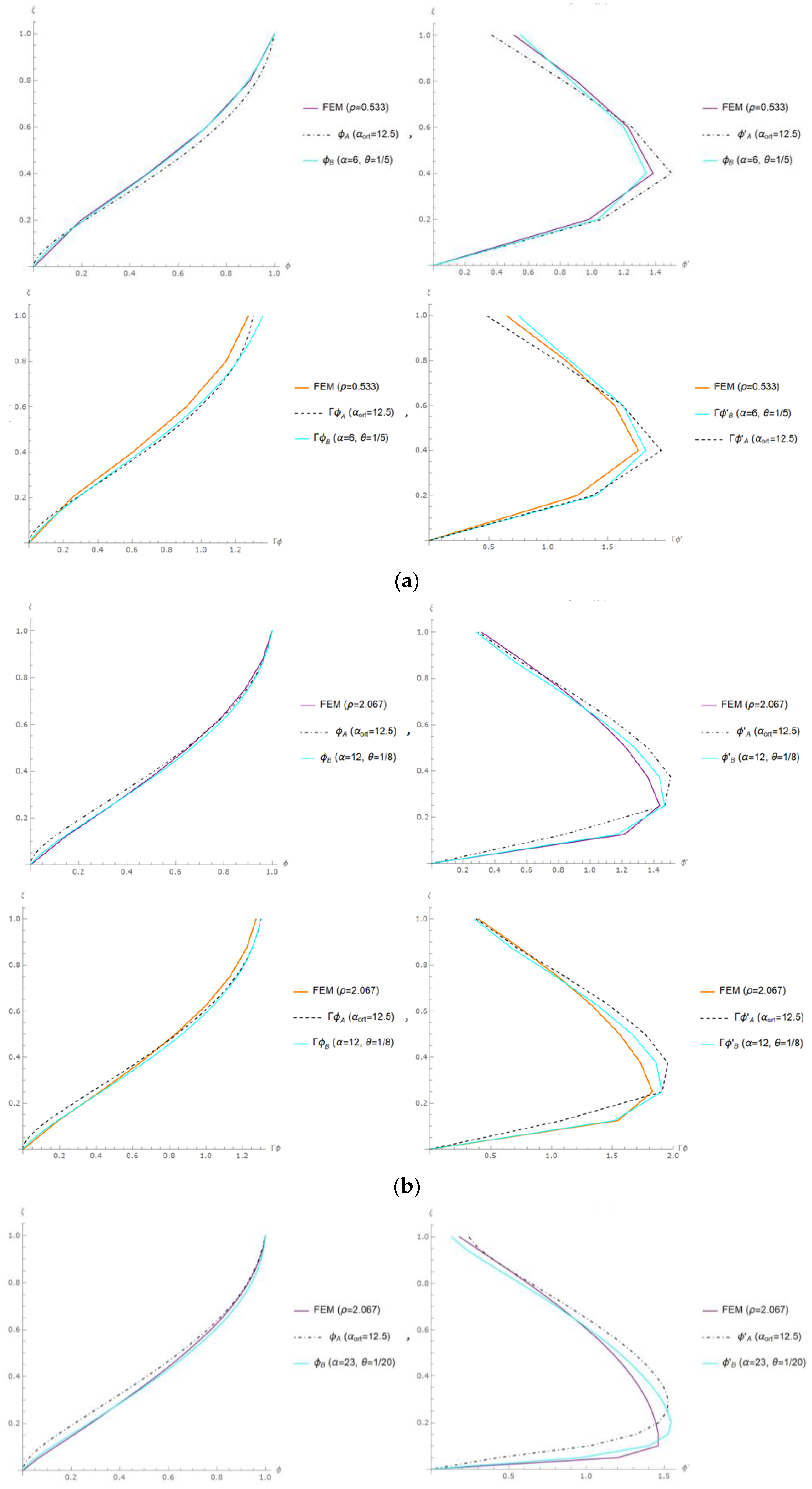
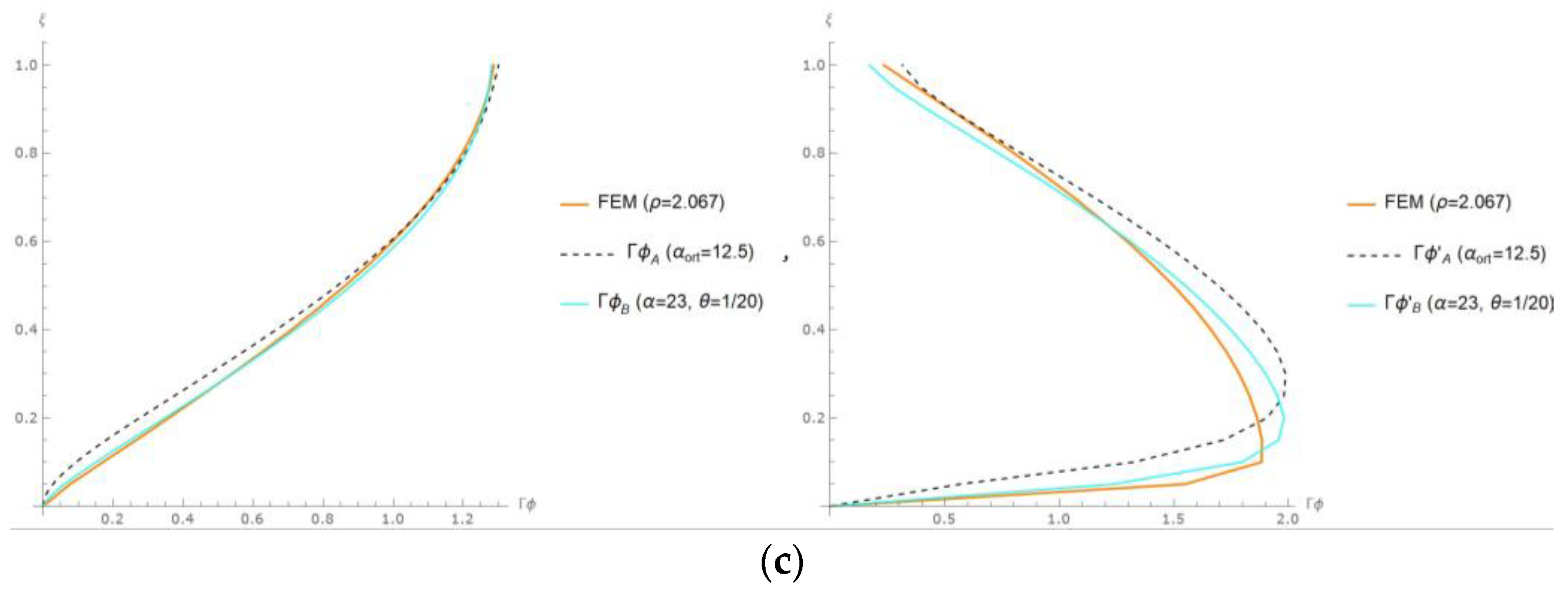
This section presents the structural responses obtained for the sample building models developed in this study, encompassing mode shape (ϕ), drift mode shape (ϕ′), modal displacement (Γϕ), and modal inter-story drift ratio (Γϕ′). These responses are graphically illustrated in
Figure 2 for multiple sample models. The results, denoted by dash-dotted black lines with an index labeled as A, depict the solutions obtained using Miranda’s approach (α = 12.5, θ = 0). The results represented by solid blue and green lines labeled as B correspond to the proposed model approach in this study (α determined through iterative experimentation, θ = 1/N), while the purple and orange lines represent the FEM results. The results for the “maximum inter-story drift ratio (IDR
max)” are also presented in the subsequent section for comparative analysis.
Estimation of Maximum Inter-Story Drift Ratios (IDRmax)
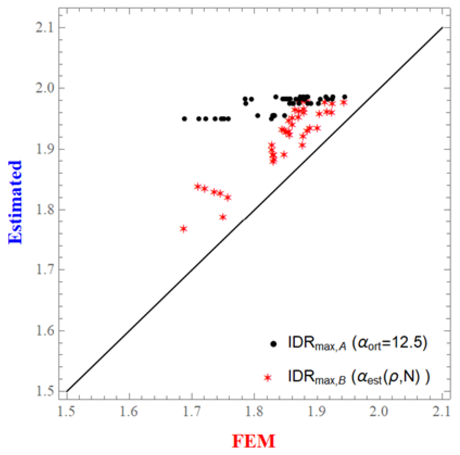
This study presents the maximum inter-story drift ratios obtained for the proposed model (θ = 1/N) and the cases where the base rotation is 0, as illustrated in
Figure 3. In particular, the lateral deformation profiles obtained using the average value of α = 12.5 recommended by Miranda’s approach (θ = 0) for frame buildings with the estimated α value for the θ = 1/N condition proposed in this study were compared. The procedures were repeated for sample-building models in each set (group), and the maximum relative inter-story drift ratios (IDR
max) were determined and compared with the SAP2000 (FEM) results. The results are compared on a one-to-one function graph provided in
Figure 3. The circular data points labeled as A in the graph represent the solution obtained using Miranda’s approach (α
ort = 12.5, θ = 0), while the starred data points labeled as B represent the proposed model approach in this study (α determined through trial and error, θ = 1/N). All predictions from the continuous model were overestimated from the SAP2000 (FEM) result values.
It can be observed that the analytical results obtained for cases where the base rotation was different from 0 significantly improved the FEM results. This improvement was particularly pronounced in low-rise models; however, as the number of stories increased, the rate of improvement diminished. This can be attributed to the fact that the base rotation decreases with respect to N and approaches 0, leading to an approximation of the fixed-end beam model solution at the base. Although continuous models are more suitable for analyzing multistory buildings, including the base rotation angle in the continuous model solution also allows for its applicability to low-story buildings.
3.3. Determination of Lateral Stiffness Ratio (α)
In the preceding section, the numerical values of lateral stiffness ratios, as defined in the proposed equations, were obtained via an iterative process employing SAP2000 simulations of building models with varying Blume ratios and floor quantities.
Figure 4 presents the graph illustrating the variation of the lateral stiffness ratio (α) for the number of floors (N) and the Blume ratio (ρ). It can be observed from the figure that α changes depending on ρ and N. The relationship linking the lateral stiffness ratio (α), the beam–column stiffness ratio (Blume coefficient) (ρ) specific to the building models, and the number of floors (N) is depicted in
Figure 4.
The variation of ρ, defined for discrete (frame) systems, significantly influenced the structural displacements. The lateral displacements increased as ρ increased, and the most significant differences in displacements occurred in the range of 0.0 to 0.125, where the fundamental mode transitioned from flexural to mixed (a combination of flexural and shear behavior). When ρ exceeded 0.125, the lateral displacements changed more gradually. Similar variations were also observed for the first mode of inter-story drift. The change in the maximum inter-story drift toward lower floors was rapid within the range of 0.0 to 0.125. In extreme cases, at ρ = 0.0, the structure behaved like a flexural beam, whereas, at ρ = ∞, it exhibited pure shear behavior, with the maximum inter-story drift occurring at the top and ground floors, respectively [
39]. These findings for moment-resisting frame systems support the relationship between the lateral stiffness ratio α and ρ. As shown in
Figure 4, the variation of α, representing the structural behavior in the continuous model, was rapid for 0.0 < ρ < 0.125 and gradually increased after ρ ≥ 0.125. Therefore, it is appropriate to consider the behavior in two sections to obtain a more accurate α.
Nonlinear regression analysis using the DataFit [
40] program was performed to estimate the equations. The relationship between the variables was investigated by defining two independent variables (ρ and N) and one dependent variable (α). The most suitable set of equations to determine α was obtained in two sections. The first Equation (21) corresponds to the range up flexural to the transition of mixed behavior, while the second Equation (22) corresponds to the range from mixed behavior to shear behavior.
When 0.0 < ρ < 0.125, a coefficient of multiple determination (R2) = 0.99 and adjusted coefficient of multiple determination (Ra2) = 0.99 were achieved. The corresponding equation constants were “a1 = 2.672”, “b1 = 0.851”, and “c1 = 0.401”.
When ρ ≥ 0.125, a coefficient of multiple determination (R2) = 0.93 and adjusted coefficient of multiple determination (Ra2) = 0.93 were achieved. The corresponding equation constants were “a2 = 0.0946”, “b2 = 0.877”, and “c2 = 2.722”.
With this proposed estimation equation, the lateral stiffness ratio of a building model can be quickly determined with minimal information from the building model. It provides more accurate results than the approximate average values commonly used in the literature and assists in estimating α without involving complex calculations for the shear stiffness expression of frame systems (GA).
4. Evaluation of the Model
This paper presents two moment-resisting frame models (
Figure 5) with distinct features for evaluating the proposed model. Detailed information regarding these models is provided below. The eigenvalue analyses of detailed finite element models are employed to calculate the dynamic characteristics of the structures, which are subsequently compared to those obtained using the approximate method proposed in this study. Furthermore, the buildings’ lateral deformation responses and inter-story drift ratio demands are determined using detailed finite element analysis under the response spectrum analysis. The simplified method compares these results to the lateral deformation demands obtained. The buildings’ two-dimensional linear finite element models were constructed utilizing the SAP2000 structural analysis software. The results obtained through the eigenvalue finite element analysis are assumed to be the “exact” results in this study.
Example 1 consisted of a three-span, five-story moment-resisting frame model. The beam–column rigidity ratio was 0.6 (ρ = 0.6), and the spans and story heights were equal, measuring 4 m and 3 m, respectively. The floor weights in the frame were uniformly distributed, with each floor weighing 800 kN. The first-mode period of vibration was 0.90 s. Dynamic analysis was performed using the UBC97 response spectrum. The lateral deformation responses and the maximum inter-story drift ratio estimations for the fundamental mode were compared between the proposed approach and the analysis; the results are shown in
Figure 6.
In Example 1, the maximum inter-story drift ratio obtained through the proposed method (α(ρ, N) = 6.1, θ = 1/5) exhibited a difference of 4.24% compared to the results obtained from the finite element model. This maximum value was observed at the corresponding height location in the SAP2000 model. When the same example was solved using Miranda’s approach (α = 12.5, θ = 0), the difference amounted to 10.51%. It can be observed that the proposed approach here yields an improvement of approximately 6% in this sample-building model. As evident from the results, when the correct α definition was employed, the proposed method captured the structural responses more accurately along the building height.
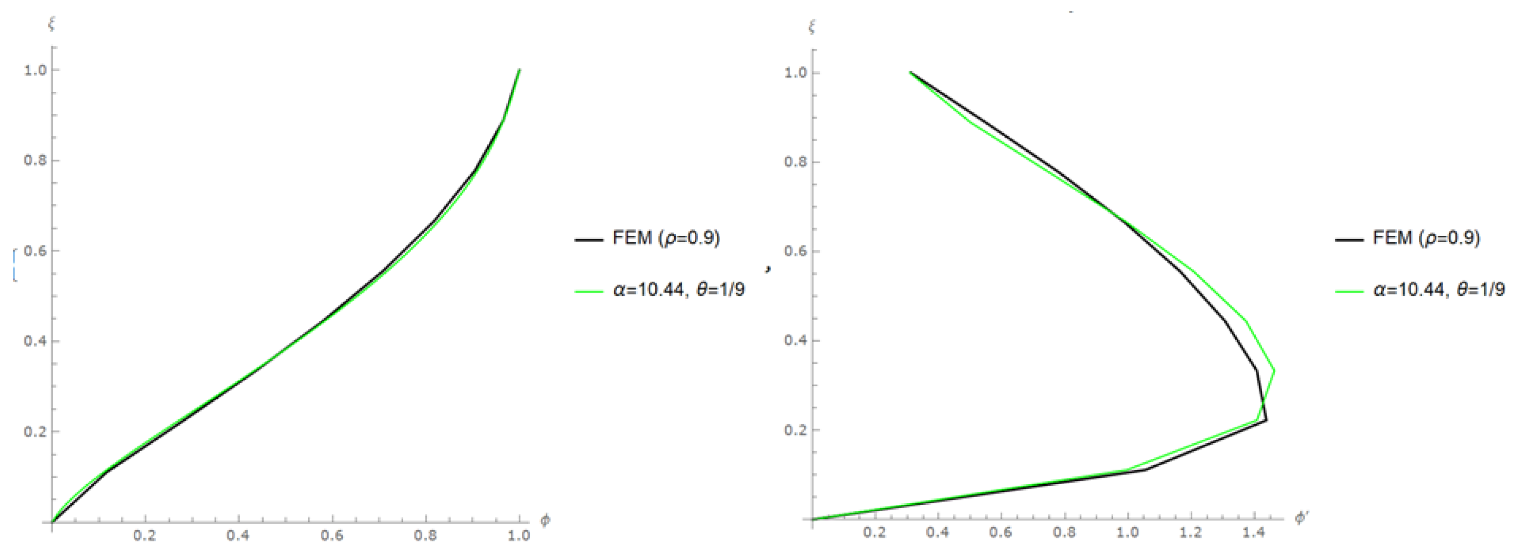
Example 2 considered a moment-resisting frame model with five spans and nine stories. The beam-to-column stiffness ratio was 0.9 (ρ = 0.9). The spans and story heights were equal in length and are 3.8 m and 3 m, respectively. The weights in the frame were equal at each story and 1200 kN. The first-mode period of vibration was 1.53 s. Dynamic analysis was performed using the UBC97 Response Spectrum. The lateral deformation responses and the maximum inter-story drift ratio estimations for the fundamental mode were compared between the proposed approach and the analysis; results are shown in
Figure 7.
For Example 2, the maximum inter-story drift ratio obtained through the proposed method (α(ρ, N) = 10.44, θ = 1/9) exhibited a difference of 3.84% compared to the results obtained from the finite element model. This maximum value was nearly observed at the corresponding height location, aligning with the results from the SAP2000 model. When applying Miranda’s approach (α = 12.5, θ = 0) to the identical example, a discrepancy of 6.94% was observed. The proposed approach demonstrated a performance enhancement of approximately 3.1% in the analyzed sample building model. This result indicates a significant influence of the θ dependent on N in Example 1, which had fewer floors. As the number of stories increased, θ approached 0, resulting in a decrease in the improvement rate, as expected.


