Non-Destructive Testing in Concrete Maturity Modeling and Master Curve Development

Abstract

Assessing concrete quality as construction goes on provides early warnings of potential flaws and leads to timely corrections in mix proportioning and placement techniques. Compressive strength and maturity modeling are among the most common parameters used by the concrete industry. Past studies indicated that non-destructive methods, NDTs, relate well to maturity and concrete strength predictions. In this study, the hydration temperature–time history of concrete was explored in defining “master curves” for concrete maturity for the first time. Well-accepted NDTs, such as ultrasonic pulse velocity and resonant frequency, were used in this effort. The study findings indicated that the novel approach of “master curves” for the maturity of concrete can be defined and follow a generalized logarithmic form. The best fit models relating NDT response and the maturity temperature–time product provided a high coefficient of determination (i.e., in almost all cases above 0.9 and p < 0.05), thus resulting in a very good fit. The shift factors for each mixture’s maturity function in relation to the master curve were related to concrete properties. The shifted maturity functions from the concrete mixtures included in the study had a perfect transition to the master curve (i.e., all the shifted data overlap the master curve trend line with an R² = 1). The NDTs’ ability to capture the hydration temperature-time history was assessed with impeded sensors into the concrete mixtures. This approach has provided strength prediction models with a high accuracy (i.e., good agreement between observed and predicted strength values with R² = 0.93). The proposed NDT-based maturity modeling through “master curve” development provides significant benefits in relation to traditional maturity modeling since it offers the opportunity to: (i) predict strength without having to repeat maturity testing each time a producer adjusts mixture proportioning to fine tune mix design; (ii) save testing time and cost due to reduced maturity evaluation from the use of master curves; and (iii) be able to quickly predict without further testing what the strength gain will be due to variations in mixture proportioning. The ability to monitor concrete maturity, and thus strength, with NDTs in reinforced concrete is of particular interest since using cores is problematic due to the presence of reinforcement.

1. Introduction & Background

Monitoring concrete quality during construction and/or production of pre-cast concrete is a critical need to provide early warnings of potential flaws and identify timely corrections in mix proportion and placement techniques. Compressive strength is among the most common quality indicators used by the concrete industry. During production, early detection implies monitoring concrete strength at early ages. Over the years, many studies have investigated the effect of various parameters (e.g., mixture proportion, cement type, curing conditions, aggregate, additives, etc.) on concrete strength. The findings have been well documented and extensively reported in standard concrete references [1,2,3]. Overall, aggregate used in concrete should have suitable strength and resistance to abrasion, chemical attack, and freezing–thawing [1,2]. When chemical admixtures are used, these are added to water during batching, and—depending on the type used—may affect setting time, hardening, water demand, workability, and entrained air among other properties [3,4]. The strength of concrete is influenced by the specific properties of all the ingredients and the water-to-cement ratio (w/c), cement type, and/or the use of supplementary cementitious materials [5,6]. Concrete permeability and air void structure are also affected by both chemical admixtures and supplemental cementitious materials, such as fly ash, slag cement, and silica fume among others [6]. In addition to compressive strength, modulus of elasticity is also a very important parameter in structural analysis and design of concrete structures. Thus, over the years, numerous studies have examined the effect of various parameters on concrete elastic modulus, its relationship to compressive strength, and the development of predictive relationships [7,8]. With the use of non-destructive testing in concrete, the relationship between static elastic modulus from destructive testing and dynamic modulus has been explored for both conventional and alternative concrete mixtures [8,9].

In recent years, the value and potential adoption of non-destructive testing in assessing concrete properties and quality during construction have been emphasized by many studies and the Federal Highway Administration (FHWA) [10,11,12]. This has generated the need to develop this study focused toward the implementation of NDTs in concrete assessment for QA and, more specifically, in maturity modeling, which is the focus of this manuscript. The benefits of using NDTs in quality assurance (QA) include faster results in relation to destructive testing and increase in testing frequency without significant increase in cost. A larger testing dataset is particularly helpful in developing accurate predictive and machine learning models. As mentioned earlier, many studies explored the development of experimental relationships between parameters obtained from NDTs, such as ultrasonic pulse velocity (UPV), with compressive strength and modulus [13,14,15,16]. The use of alternative NDTs was also considered in developing models for predicting the static elastic modulus [17,18]. Amini et al. [19] presented statistical univariate and multivariable regression models to predict the compressive strength of concrete using UPV and rebound hammer measurements. The results of this and other studies showed that in some instances the accuracy of the models when considering multiple NDTs are higher [19,20]. Kewalramani et al. [21] successfully employed linear regression and an artificial neural network (ANN) to predict the compressive strength of UPV. Similar studies in recent years have developed alternative machine learning models for predicting compressive strength of concrete using available mixture optimization data [22,23].

The value of using alternative NDTs and/or blended methods for assessing concrete properties was highlighted by various researchers [19,20], thus paving the way and emphasizing the need for this study. In terms of alternative NDTs, Chávez-García et al. [17] developed a relationship between static elastic modulus from destructive testing and dynamic elastic modulus from non-destructive tests, such as UPV, electrical resistivity, and resonant frequency testing. Lee et al. [24] performed a series of experimental and numerical analyses to find the most robust relationship between static modulus of elasticity and dynamic modulus of concrete obtained from UPV and resonant frequency. The use of non-destructive testing is advantageous since the same samples and/or concrete members can be tested again and again for assessing concrete quality in terms of uniformity and strength gain with regards to the expected values. As concluded earlier, past studies indicated that ultrasonic pulse velocity (UPV) and the corresponding dynamic modulus of elasticity relate well to the compressive strength and modulus of elasticity from static destructive compressive strength testing [25,26]. Thus, such parameters from NDT evaluation can be used as quality control measures during concrete production [25]. In order to estimate concrete strength—and thus modulus—with hardening age, the concept of maturity is used by the concrete community and industry in developing predictive models. Temperature and time are two important parameters considered in this modeling approach [14,26]. The Nurse–Saul maturity function (MI(t)) equation presented later in the manuscript represents the relationship between concrete temperature, time, and strength gain. The resulting maturity index (MI) (i.e., sum of the product of time and temperature history during the hydration process) can be calculated in real time in the lab and/or the field. While curing conditions during hydration affect strength gain [5,27] according to the maturity function, concrete of the same mix that has the same maturity index has approximately the same strength whatever combination of temperature and time is experienced. Maturity models are mixture-specific since the hydration rate in concrete is dependent on mixture ingredients and proportioning [26,28,29,30].

Thus, based on past studies’ shortcomings and recommendations [20,26,28], it was the objective of this study to explore alternative non-destructive-based testing, such as ultrasonic pulse velocity and resonant frequency, to model maturity of concrete at young ages after casting. Maturity represents the effect of time and temperature during hydration on concrete strength gain. The relationship between concrete quality measures (e.g., compressive strength, UPV, or modulus of elasticity) and maturity index (MI) is mixture-specific [26,28,29,31]. Thus, to overcome the extended maturity testing needed each time a new mixture is developed, it was the second objective of the study to explore for the first time ever a novel approach in maturity modeling by developing “master curves” for a group of concrete mixtures. This novelty in maturity modeling includes (i) the development of a representative maturity function (identified herein as “master curve”) for a group of concrete mixtures with similar ingredients and proportioning and (ii) define the transfer function between individual mixture MI relationships and the “master curve” in function of mixture properties. The benefits of developing the novel concept of universal functions for similar mixtures is driven from the potential benefits to the concrete industry in predicting strength without having to repeat maturity testing each time a producer adjusts mixture proportioning to fine tune mix design; being able to quickly predict what will be the strength gain for small variations in mixture proportioning; and saving time and testing cost by reducing maturity testing in such conditions. For example, a producer could assess how variations in material and mixture proportioning will affect (i) fresh concrete properties, such as unit weight and air content, combined with (ii) UPV response and/or initial strength at early ages to predict concrete strength and/or dynamic modulus over time during the hydration at later ages. To achieve this, once the “master curve” and shift factor equations are defined for a specific set of concrete mixtures, trial batches could be produced during mix design and/or the concrete optimization phase to assess impact on fresh concrete properties and NDT response early on in order to estimate strength and modulus at later ages. This will reduce the need for the traditional ongoing shortcoming of maturity monitoring requiring extensive testing during concrete hardening and/or hydration over time when a mixture is modified or a new mixture is explored [14,20,25]. Such early assessment will also provide early warning on the potential implications of changes and/or variability in materials and proportioning without having to wait for follow-up testing during longer periods of hydration [14]. At the same time, such early assessment will minimize the need for ongoing monitoring of hydration and strength gain during concrete production, thus saving time and reducing testing needs. Thus, during concrete production, the use of master curves could minimize quality control testing for (i) assessing production quality and assess early impact on concrete strength at later ages as well as (ii) assess whether the 28-day design target strength is expected to be achieved based on limited testing early on. In terms of field evaluation during construction of a concrete structure, companion cylinders are often used for monitoring maturity and strength gain in time, as these are affected by similar field conditions as the structure. Such companion cylinders, along with the fresh concrete properties regularly monitored during concrete batching, could be used similarly to the lab testing case to assess from early ages what will be the follow-up implications in strength and modulus due to potential variability in production concrete uniformity as construction goes on. Such companion cylinders, and/or selected structural members, could be tested with UPV for verification as well. These early warnings could be beneficial in adjusting concrete mix materials, proportioning during the construction of the structure, or making sure that targeted values of strength are achieved.

In a previous effort, the relationships between UPV and dynamic modulus with the temperature–time factor (maturity index) were investigated with a single concrete mixture [28]. The results showed that such relationships were dependent on mixture composition. In this study, the results of UPV, resonant frequency, and compressive strength of eleven concrete mixtures were investigated to identify (i) whether a “master curve” for a group of concrete mixtures is possible, (ii) the general predictive form of such a curve, and (iii) whether a transfer function for shifting the individual maturity curves to the “master curve” can be defined using mixture properties.

It should be mentioned that objective of this study was to (i) propose an NDT-based maturity approach for the specific and/or typical concrete mixtures encountered in infrastructure projects in the region rather than a universal maturity study for all possible concretes and to (ii) assess whether the novel concept of “master curves” for maturity can by developed. Since “maturity” is mixture-specific, calibration of maturity models is needed when other concrete mixtures are of interest (such as fiber-reinforced, low-shrinkage, self-consolidated, high-volume fly ash, etc.). As mentioned earlier, this second goal represents a novel approach in maturity modeling for the first time ever suggested by developing “master curves” and thus overcoming the traditional and extended maturity testing needed each time when a new mixture is developed with similar concrete ingredients. Additionally, the successful development of the transfer functions between individual mixture MI relationships and the “master curve,” in the function of mixture properties, represents a useful and innovative approach in considering mixture variations and eventually expanding the suggested modeling approach to other mixture types.

2. Materials and Methods

In this study, two NDTs were used: ultrasonic pulse velocity and resonant frequency. While UPV can be used in both lab and field conditions, resonant frequency is primarily for lab samples and is thus a complementary method when further forensic verification may be of interest.

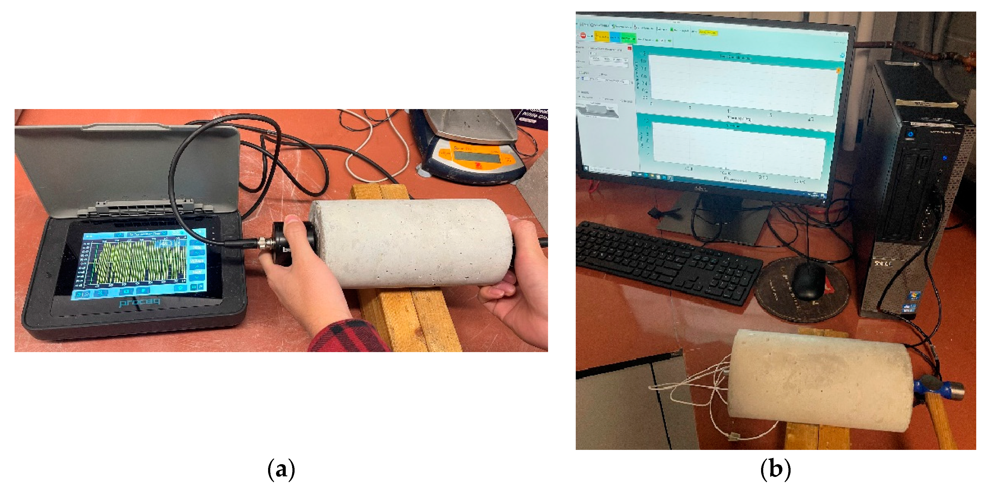
UPV transducers measure the wave’s propagation time through concrete. Three modes of testing are possible, direct, semi-direct, and indirect transmission. In the direct method used in this study, longitudinal compressive stress waves generated by an electro-acoustic transducer travel through the concrete and are received at the other end by another transducer, Figure 1a. As per ASTM C597, the pulse velocity is independent of the sample dimensions when there are no reflected waves from the sample boundaries [32]. This is assured when the smaller sample dimension exceeds the signal wavelength. With the distance between the two transducers known, the velocity can be calculated. The velocity of compression waves in concrete is related to concrete’s elastic properties and density. Equation (1) provides the relationship between concrete properties and compression wave velocity [32], while Equation (2) provides the dynamic modulus, $E_d$, in relation to pulse velocity and concrete properties:

$$V=\sqrt{\frac{E_d(1-\nu )}{p(1+\nu )(1-2\nu )}}$$

(1)

$$E_d=\frac{(1+\nu )(1-2\nu )}{(1-\nu )}\rho V^2$$

(2)

where $E_d$ is the dynamic modulus of elasticity, N/m², $\nu$ is the dynamic Poisson’s ratio, $\rho$ is the density, kg/m³, and V is the ultrasonic pulse velocity, m/s. The UPV configuration used in this study was in the direct longitudinal mode, Figure 1a.

Resonant frequency testing, RFT, involves determining the fundamental resonant frequency of concrete samples. Similarly to UPV, the fundamental longitudinal, transverse, and torsional frequencies can be determined. Two testing alternatives are available—the forced and the impact resonance methods. In this study, the impact resonance method was used in the longitudinal testing mode, in which the specimen is struck with a small impactor at one end and the response is measured with an accelerometer at the other end of the sample. The maximum amplitude observed represents the resonance frequency. RTF is more sensitive to sample size (i.e., cylinders with length-to-diameter ratios equal to 2 are often recommended even though ASTM C215 recommends a higher ratio). The resonant frequency is a function of sample’s elastic constants (modulus and Poisson’s ratio), geometry, and mass density [14,33]. The dynamic modulus of a concrete sample in the longitudinal mode used in this study is calculated based on the fundamental longitudinal frequency and a sample shape constant based on Equation (3) [34]:

$$E_d=DM {(n\prime )}^2$$

(3)

where E_d is the dynamic modulus in Pa; $n^{\prime }$ is the fundamental longitudinal frequency in Hz; D is 5.093 ($\frac{L}{d^2}$) in ${\mathrm{m}}^{-1}$ for a cylinder or 4 ($\frac{L}{bt}$) in ${\mathrm{m}}^{-1}$ for a prism; and M is the mass in kg. The configuration of the resonance testing gauge (RTG) used in this study for resonance frequency evaluation is shown in Figure 1b.

In this study eleven mixtures were considered,

Table 1. Concrete mix proportion and properties.

Mixtures	WAEA/Wcement	WHRWR/Wcement	Fresh Unit Weight (kg)	w/c	Air Content	Slump (mm)	Average 28-Day Compressive Strength (MPa)
Mix 1	0.16%	0.11%	2352	0.44	4.0%	25	38
Mix 2	0.40%	0.24%	2418	0.44	3.6%	15	31
Mix 3	0.40%	0.24%	2274	0.45	6.5%	98	31
Mix 4	0.40%	0.24%	2336	0.43	4.6%	111	31
Mix 5	0.40%	0.24%	2287	0.45	5.4%	76	25
Mix 6	0.40%	0.24%	2271	0.45	6.0%	146	22
Mix 7	0.40%	0.24%	2278	0.45	5.8%	105	23
Mix 8	0.40%	0.24%	2271	0.45	6.1%	76	25
Mix 9	0.40%	0.24%	2253	0.48	6.2%	130	19
Mix 10	0.40%	0.32%	2258	0.48	5.4%	175	25
Mix 11	0.40%	0.40%	2232	0.50	5.6%	226	26

Note: HRWR = high-range water reducer; AEA = air-entrainer agent; all mixtures designed based on the departure concrete mix (i.e., meeting MD7 designation) designed according to ACI 211 and with proportioning of 1014 and 733 kg of coarse and fine aggregate, respectively, and 378 kg of type I Portland cement per m³ of concrete. Water and admixture contents were adjusted as reported herein.

. Some of these mixtures represent typical concrete used in the construction of infrastructure projects in the region (Mixes 1 to 8), reflecting possible fine-tuning in proportioning that a concrete producer may consider. The remaining mixtures have higher water-to-cement ratios, deviating from a typical concrete in the region (Mixes 9 to 11). The typical mixtures have to meet proportioning and acceptance requirements similar to MD7 (Maryland designation 7). The deviation from MD7 was intentional in order to observe the effect of different parameters on NDT response and assess the feasibility of the “master curve” concept. A subset of these mixtures could also represent potential mixture proportioning variability during production with regards to water-to-cement ratio. The concrete ingredients included a 0.78 mm trap rock #57 aggregate and fine aggregate—meeting ASTM C33, Type I cement, water, and admixtures such as air-entraining admixture (AEA)—and high-range water reducer (HRWR), meeting AASHTO M 154 and M194, respectively. Air-entraining admixtures provide resistance to freeze–thaw, although they lead to a reduction in strength. High-range water reducers provide the desired concrete strength at a lower water content with acceptable workability [7].

Cylinders with diameters of D = 100 mm and heights of L = 200 mm were prepared from each mixture and tested with UPV and RFT and for compressive strength at different hardening ages. The samples were kept in a water bath at room temperature during curing. iButton sensors were embedded in companion samples for each mixture for recording the temperature history during hydration. The temperature history was then used to calculate the temperature–time factor using the Nurse–Saul maturity function [35]:

$$MI(t)=\sum (T_a-T_o)\Delta t$$

(4)

where MI(t) is the temperature–time factor at age t, degree days or degree hours; ∆t is time interval, days or hours; $T_a \mathrm{a}\mathrm{n}\mathrm{d} T_o$ are the average concrete temperature during the time interval ∆t and the datum temperature, respectively, in °C. The datum temperature is the temperature below which the chemical reaction between cement particles and water ceases. It is the theoretical temperature below which concrete ceases to gain maturity. Even though a procedure is available in ASTM C1074 to determine such temperature experimentally, the standard recommends a datum temperature of 0 °C for concrete with no special admixtures or supplemental cementitious materials, as is the case in this study. Thus, the datum temperature was assumed to be zero [25,26]. The samples were tested with UPV and RFT 1, 3, 7, 14, and 28 days after casting, and compressive strength was tested for three specimens at each age.

Once concrete mixing is complete, the hydration chemical reaction takes place between concrete ingredients. More specifically, during the initial mixing phase, a reaction takes place when cement and water particles come into contact [6]. The aluminate compounds react with water molecules to form ettringite. The energy released from such exothermic reaction causes an initial peak in temperature at early ages and, depending on the mixture, as early as a few minutes to hours depending on the mixture and concrete ingredients [14,25,26]. During the next hydration phase, a surface coating of the cement particles occurs. As this coating keeps increasing, it slows down the hydration reaction. The amount of hydrated concrete keeps increasing steadily while it stays in a fluid form. The length of time for this phase depends on the specific concrete mix. In the next phase of hydration, the tricalcium and dicalcium silicates react, producing an increase in internal temperature and the formation of silicate hydrate (CSH), associated with strength gain. This phase is followed by a reduction of unhydrated free particles and thus a slowdown in temperature increase. After this stage, the hydration process continues to slow until complete hydration of the remaining unhydrated cement particles is achieved. Hydration is often not complete when the concrete reaches the desired strength, but it continues—if curing conditions are favorable—in some cases for more than a year, and under unfavorable conditions, it stops before reaching completion.

Based on the maturity modeling testing outlined in ASTM C1074 [35], concrete hydration and the development of the Maturity Index, are monitored by using the standard laboratory curing conditions (i.e., 20 ± 2 °C, and relative humidity of 100%). As identified in the standard, the definition of maturity is “concrete experiencing the same product of time-temperature history, no matter what the specific temperature pattern occurred,” will produce the same MI(t), Equation (4), and thus will produce the same strength. Thus, whether specific lab and/or field conditions are considered, as far as the product MI(t) is the same, concrete will have reached the same strength even though the temperature history might be different. Similarly, since the degree of moisture present will affect hydration and thus concrete temperature history, such effects are also accounted for. The trend of time–temperature will only affect how fast in time a specific strength will be achieved in relation to each case.

3. Results

As mentioned previously, the maturity index (MI) is mixture-specific. While several alternative relationships were explored for relating NDT response to the maturity temperature–time product, it was concluded that the best fit model was of the logarithmic form $y=a ln\left(x\right)+b$ [28]. For all 11 mixtures included in this study, the logarithmic form also provided the best fit. The corresponding R² are shown in

Table 2. R² for best fit logarithmic models between NDTs and compressive strength with temperature–time.

Mix	UPV vs. Temp-Time	Ed (RTG) vs. Temp-Time	Compressive Strength vs. Temp-Time
1	0.99	0.95	0.97
2	0.95	0.97	0.95
3	0.86	0.97	NA *
4	0.96	0.96	NA *
5	0.92	0.97	0.98
6	0.96	0.96	0.99
7	0.97	0.95	0.92
8	0.92	0.97	0.90
9	0.94	0.95	0.98
10	0.99	0.99	0.99
11	0.95	0.96	0.99

* Limited data; p < 0.05 for all cases.

. The R² for almost all cases was above 0.9 and p < 0.05, indicating (i) a very good fit between NDTs and the maturity temperature–time product and (ii) consistent model forms for all concrete mixtures. It should be mentioned that such NDTs provide consistent response in concrete independent of the sample’s dimensions and shape [33] since these effects are factored in Equations (1)–(3). Also of note is that for Mixtures 3 and 4, there were not sufficient compressive strength data to provide reliable relationships. The consistency on the model form between mixtures implied that the “master curve” concept may potentially be feasible for UPV and/or dynamic modulus versus MI for a group of similar concrete mixtures. The shift function for each mixture-specific maturity equation to the generalized form (i.e., master curve) was then developed in function of mixture-specific concrete ingredients and proportioning.

3.1. Developing Master Curves for UPV and Dynamic Modulus

In order to develop the maturity master curves for UPV and/or dynamic modulus the following steps were followed:

• Using the general logarithmic form, $y=a ln\left(MI\right)+b$, the coefficients of ln(MI), “a” and/or “a′”, were set to a constant value (i.e., a = average of coefficient “a” and “a′” of all mixture equations). New coefficients “b” and/or “b′” for each mixture were then calculated. The resulting R² values are reported in

  Table 3. Modified equations of best fit for each mixture.

  Mix No.	UPV vs. Temp-Time (y = a * Ln (x) + b)		Ed (RTG) vs. Temp-Time (y = a′ ** Ln (x) + b′)
  	b	R2	b	R2
  1	2915.7	0.82	16.86	0.95
  2	3243.0	0.95	22.17	0.97
  3	3131.8	0.91	18.42	0.96
  4	3299.8	0.96	21.44	0.95
  5	3089.6	0.92	17.38	0.97
  6	3107.0	0.96	16.82	0.96
  7	3197.9	0.97	18.42	0.95
  8	3128.1	0.92	17.09	0.97
  9	3009.0	0.94	13.45	0.95
  10	3233.5	0.99	17.73	0.99
  11	3288.1	0.95	17.44	0.96

  * a = 224.26; ** a′ = 2.5; p < 0.05 for all cases.

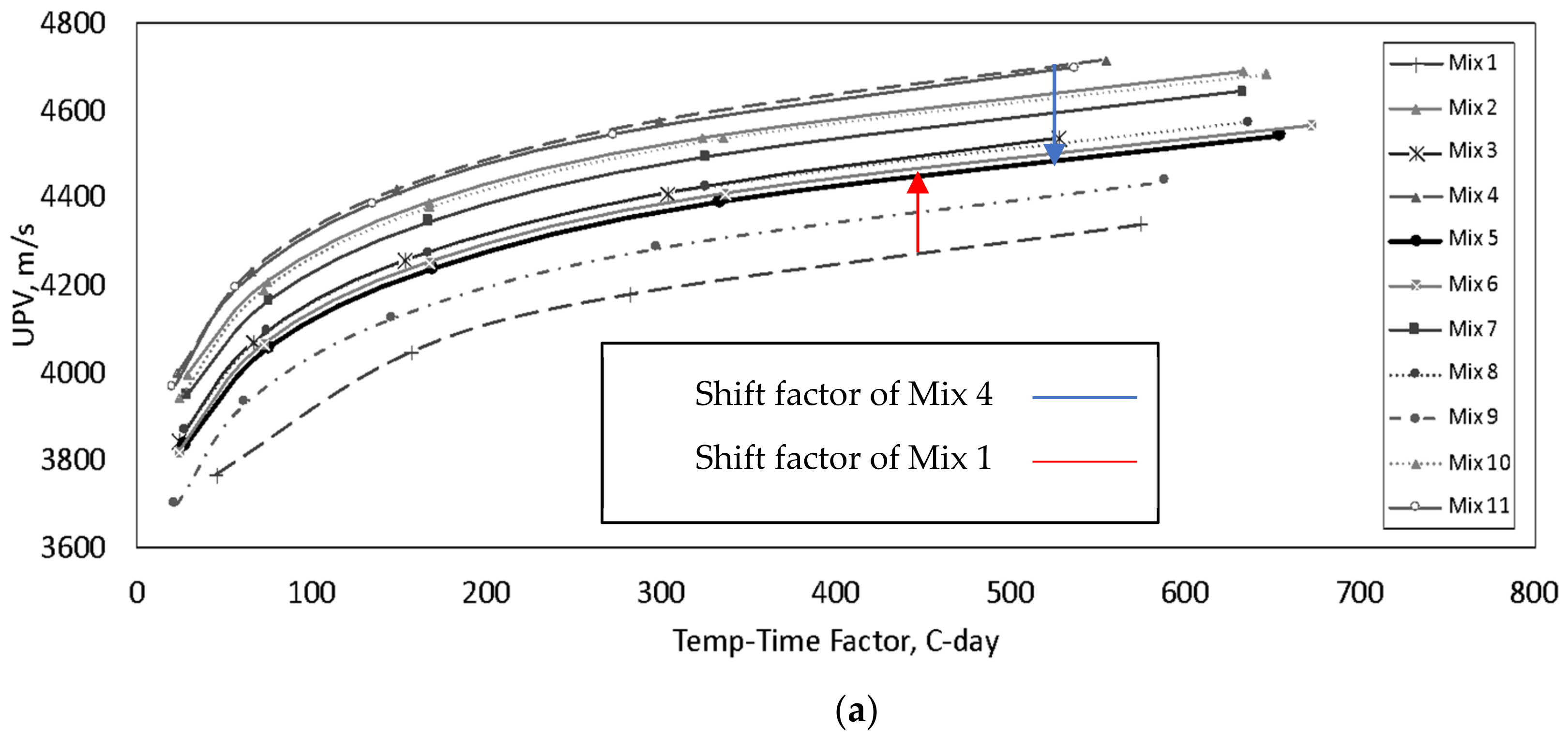
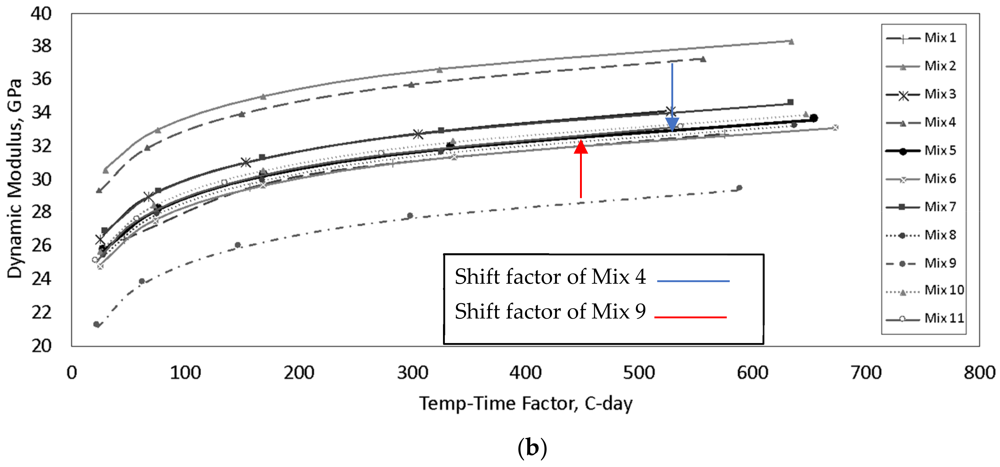
  , while the corresponding relationships for all the mixes are shown in Figure 2.
• In the next step, one mixture was selected as the reference mixture. As can be seen from Figure 2, Mix 5 represents a typical mixture used in Maryland for infrastructure projects, identified as MD 7, with test results very close to the center of all mixtures. Therefore, Mix 5 was selected as the reference mixture.
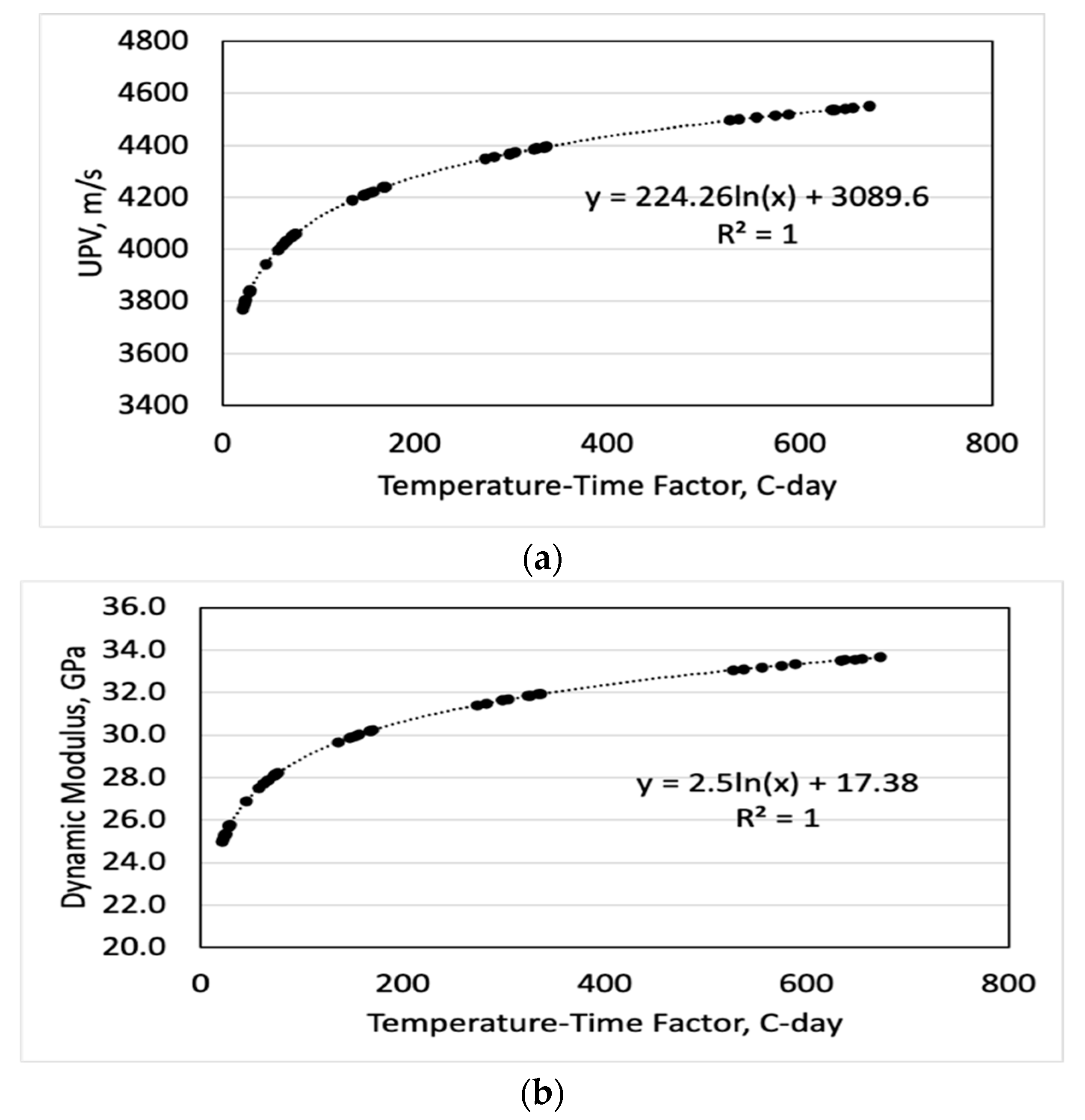
• The vertical shift factors, which are the differences between the intercepts of the governing equations of any mixture and the reference mixture (Mix 5), were calculated. Examples are shown in Figure 2. The resulting master curves from shifting are shown in Figure 3 for both the dynamic modulus and UPV.
• In the next step, the shift factors were related to concrete mixture properties. The characteristics of a concrete mix most related to the shift factor were identified based on Pearson’s correlation analysis.

  Table 4. Shift factors with concrete properties and hydration temperature.

  Mix	Shift Factor (Ed)	Shift Factor (UPV)	Initial Temperature	Slump	Average Temperature	Air Content	Unit Weight	W-C Ratio	Compressive Strength
  1	0.52	173.90	25.30	25	20.50	0.040	2352	0.44	38.00
  2	−4.70	−156.90	26.80	15	22.90	0.036	2418	0.44	30.83
  3	−0.98	−38.57	17.00	98	21.99	0.065	2274	0.45	30.96
  4	−4.02	−181.88	16.00	111	21.70	0.046	2336	0.43	30.48
  5	0.00	0.00	24.00	76	23.38	0.054	2287	0.45	25.26
  6	0.56	−21.19	23.30	146	23.43	0.060	2271	0.45	22.42
  7	−1.00	−107.98	23.00	105	22.62	0.058	2278	0.45	23.00
  8	0.45	−28.90	23.50	76	22.75	0.061	2271	0.45	25.3
  9	3.98	77.53	16.50	130	21.80	0.062	2253	0.48	19.24
  10	−0.24	−142.04	16.00	175	21.47	0.054	2258	0.48	25.36
  11	0.02	−199.82	15.00	226	19.94	0.056	2232	0.50	26.51

  includes the shift factors of each concrete mixture along with the concrete properties and the hydration temperatures during curing. The Pearson’s correlation coefficients are summarized in

  Table 5. Pearson’s correlation coefficient for shift factors based on mixture properties.

  Mix Properties	Shift Factor (UPV)	Shift Factor (Ed)
  Initial Temperature	0.38	−0.19
  Slump	−0.42	0.33
  Average Temperature	0.03	−0.14
  Air Content	0.08	0.60
  Unit Weight	0.00	−0.69
  W-C Ratio	−0.15	0.54
  Compressive Strength	0.12	−0.49

  . The parameters with higher absolute values of Pearson’s correlation coefficients were selected to be the best predictors of the shift factors. Linear regression multivariate analysis was then used to identify the relationship describing the shift factor, Equation (5):

$$y={\beta }_0+X_1{\beta }_1+X_2{\beta }_2+X_3{\beta }_3+\epsilon$$

(5)

where y is the response variable, x is the independent variable (predictor), $\beta$ is the unknown parameter, and $\epsilon$ is the residual. In a linear model, the parameters enter linearly. However, the predictors themselves do not have to be linear. Here, the objective is finding $\overrightarrow{\beta }$ (i.e., ${\beta }_0$, ${\beta }_1$, ${\beta }_2$, and ${\beta }_3$) in order to minimize the residual error ($\epsilon$). Further details can be found in Faraway [36]. Bivariate analysis on the shift factors and each one of these selected variables indicated that the best relationships have polynomial. To describe the shift factors, polynomial relationships (second degree) for each shift factor (UPV or dynamic modulus) are presented in

Table 6. Models for predicting UPV shift factor.

Model	Coefficients									Performance
	Intercept	Compressive Strength		Unit Weight		Air Content		Average Temperature		R2	RSE	p-Value
		a *	b *	a	b	a	b	a	b
1	−59.81	426.79	464.11	134.62	−392.67	−36.75	−42.21	−35.93	395.65	0.95	60.8	0.19
2	−59.81	357.91	229.99	0	0	−14.40	176.97	54.71	154.53	0.91	57.06	0.05
3	−59.81	137.77	−169.0	−349.81	−714.24	479.38	−738.61	0	0	0.81	80.88	0.16

* The equations are in the form of ax² + bx.

and

Table 7. Models for predicting dynamic modulus shift factor.

Model	Coefficients									Performance
	Intercept	Compressive Strength		Unit Weight		Air Content		W-C Ratio		R2	RSE	p-Value
		a *	b *	a	b	a	b	a	b
1	−0.55	3.72	−1.36	−0.80	−10.80	2.91	−6.30	−1.34	−0.56	0.94	1.32	0.23
2	−0.55	1.73	−5.33	−5.32	−19.85	9.14	−16.97	0	0	0.93	1.01	0.03
3	−0.55	4.6	0.28	0.51	−4.51	0	0	−1.45	0.48	0.94	0.94	0.02
4	−0.55	4.95	−0.41	0.47	−4.82	0	0	0	0	0.91	0.90	0.003

* The equations are in the form of ax² + bx.

. In selecting the best models, R-squared, p-value, residual standard error, and simplicity of the model are considered (i.e., highest R-square and p-value less than 0.05). Residual standard error (RSE), also known as the model sigma, is a variant of the RMSE (root-mean-squared error) attuned for the number of predictors in the model. The lower the RSE, the better the model. In practice, the difference between RMSE and RSE is very minor, especially for large multivariate data. The resulting models are presented in Table 6 and Table 7 and the following equations:

$${\delta }_{UPV}=357.91{\left(CS\right)}^2+229.99CS-14.4A^2+176.97A-54.71T^2+154.53T-59.81$$

(6)

$${\delta }_{DM}=4.6({CS)}^2+0.28CS+0.5{1\left(UW\right)}^2-4.51UW-1.45{WC}^2+0.48WC-0.55$$

(7)

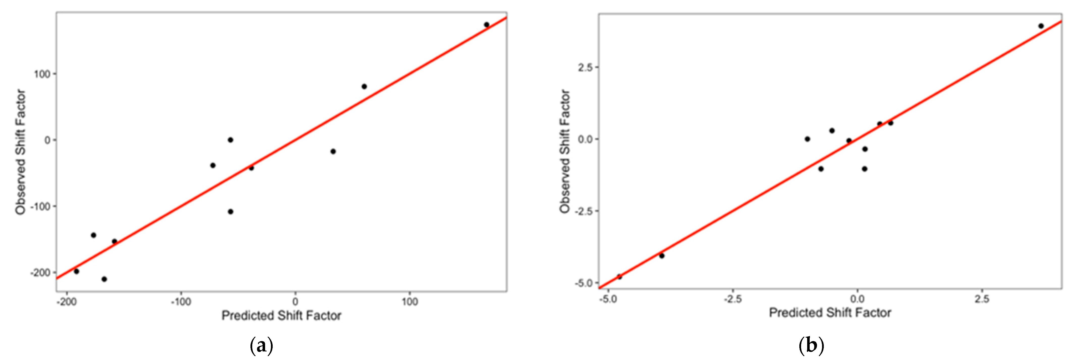
where ${\delta }_{DM}$ and ${\delta }_{UPV}$ are the shift factors for the dynamic modulus, E_d (RTG) and UPV, respectively; CS is the compressive strength in MPa; UW is the unit weight (Kg/m³); A is the air content (%); T is the average concrete temperature (°C) during the curing period; and WC is the water–cement ratio. As can be observed from the results, the prediction accuracies for the selected models were 91% and 94% for the UPV and the dynamic modulus shift factor cases, respectively.

In Figure 4, the predicted shift factors of UPV and dynamic modulus are compared with the actual values. Since data from eleven mixtures were used in relation to the number of variables in the shift functions, some deviations from the line of equality (y = x) were expected. Nevertheless, overall, there is good agreement between predicted and actual values (values close to the 45° line of equality). In fact, this is reflected in the developed master curves presented in Figure 3, in which all the shifted data are on the trend lines (R² = 1).

3.2. Compressive Strength Modeling

Experimental relationships between compressive strength and NDT response (i.e., UPV or dynamic modulus) have been explored in past studies included in the literature [13,14,15,16,19]. The response of selected models from the literature with the data from this study are presented in

Table 8. RMSE of compressive strength prediction models.

Study	Amini et al. (2019) [19]	Turgut (2004) [15]	Tanyidizi et al. (2008) [16]	Qasrawi (2000) [13]	Malhotra and Carino (2003) [14]
Model	$CS=0.7237e^{0.8V}$	$CS=0.0872e^{1.29V}$	$CS=0.2291V^2+5.939V+0.258$	$CS=36.72V-129.077$	$CS=33V-109.6$
RMSE	5.16	6.21	9.52	10.52	12.16

CS = Compressive strength (MPa), V = UPV (km/s), n = 41.

along with the corresponding root-mean-squared error (RMSE). The purpose of the analysis presented in Table 8 was to verify the model form (i.e., non-linearity) between compressive strength and pulse velocity. It should be mentioned that some of these models were developed with data from specific mixtures. For example, Tanyidizi et al. [16] developed the relationship for self-consolidating concrete (SCC). The lower RMSEs of the Amini et al. [19] and Turgut [15] models indicate that the relationship between compressive strength and UPV is non-linear, thus confirming earlier findings by Tharmaratnam et al. [37].

In this study, the testing results of the concrete mixtures at different ages were used to develop a multivariate relationship between compressive strength with UPV, dynamic modulus from RFT, and the temperature–time product. As mentioned earlier, past studies also recommended that more robust prediction models may be obtained when the results from multiple testing methods are combined [19,38]. Linear regression was employed to identify the best fit considering the following: higher R², lower p-value, residual standard error, AIC (Akaike’s information criteria), and BIC (Bayesian information criteria). AIC and BIC are indices representing the complexity of a model, with higher AIC and BIC representing higher levels of complexity. Generally, a simple model form may be more desirable and practical in terms of simple computational calculations. Some of the models with higher performances are presented in

Table 9. Models for predicting compressive strength.

Term	Model 1	Model 2	Model 3	Model 4
Coefficient
Intercept	−23.01	−49.79	−18.65	30.92
Temp–Time	0.00298	-	-	-
Ln (Temp–Time)	-	1.38	1.35	1.36
UPV	0.00047	-	−0.0016	-
Ln (UPV)	-	−8.76	-	−6.76
Dynamic Modulus	1.34	-	1.29	1.29
Ln (Dynamic Modulus)	-	40.11	-	-
Model Performance
R2	0.92	0.91	0.92	0.93
Standard Residual Error	1.99	2.13	1.91	1.91
RMSE	1.89	2.02	1.81	1.81
p-value	3.73 × 10−20	4.37 × 10−19	7.56 × 10−21	7.21 × 10−21
AIC	178.63	184.10	175.08	174.98
BIC	187.20	192.67	183.65	183.55

.

Considering all aforementioned factors, Model 4 seems to be a model better representing the data, as shown in Equation (8):

$$CS=1.36 ln\left(MI\right)-6.76ln \left(V\right)+1.29DM+30.92$$

(8)

where CS is compressive strength (MPa); MI is maturity index (temperature–time factor), °C-day; V is UPV, m/s; and DM is dynamic modulus of elasticity from RFT in GPa.

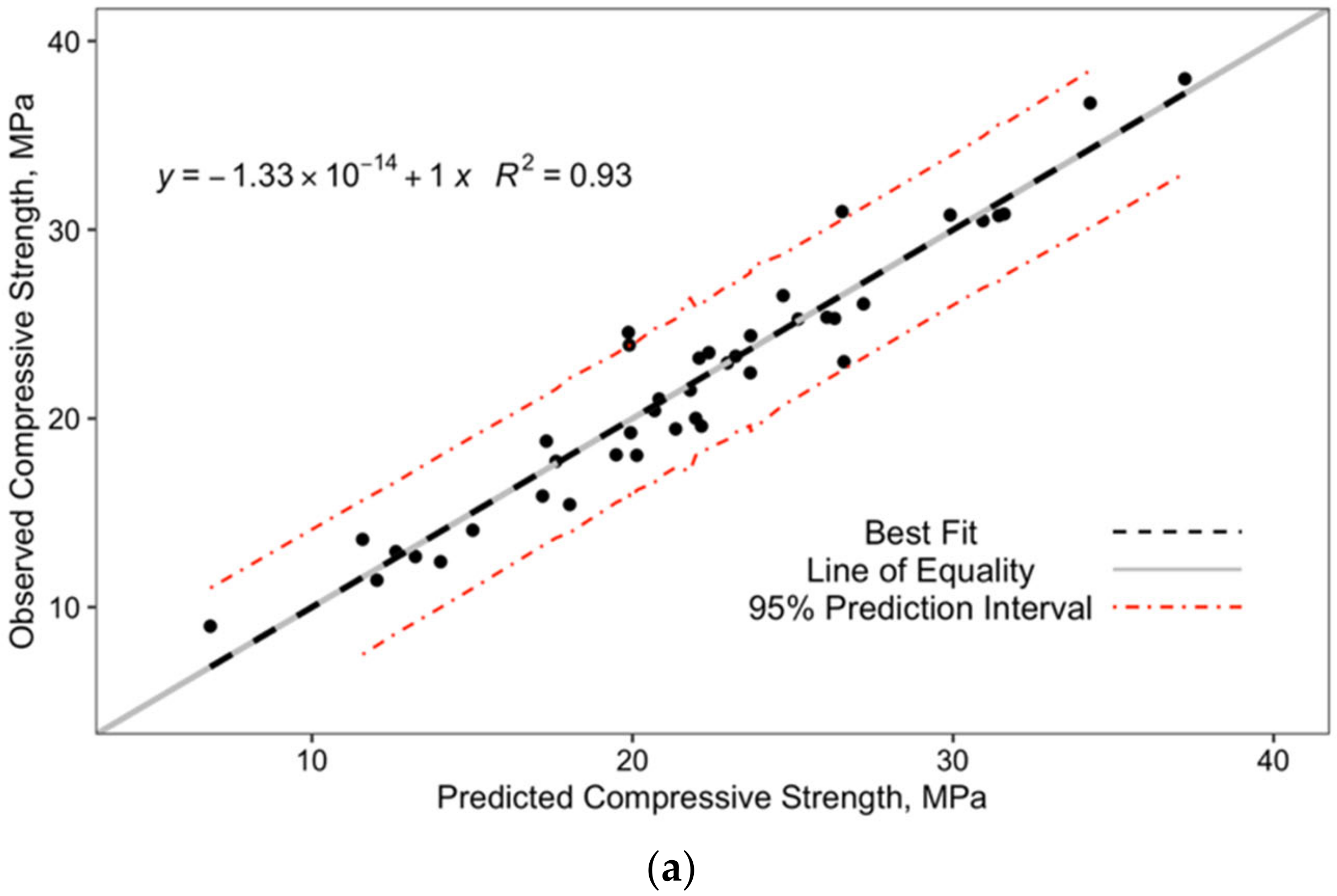
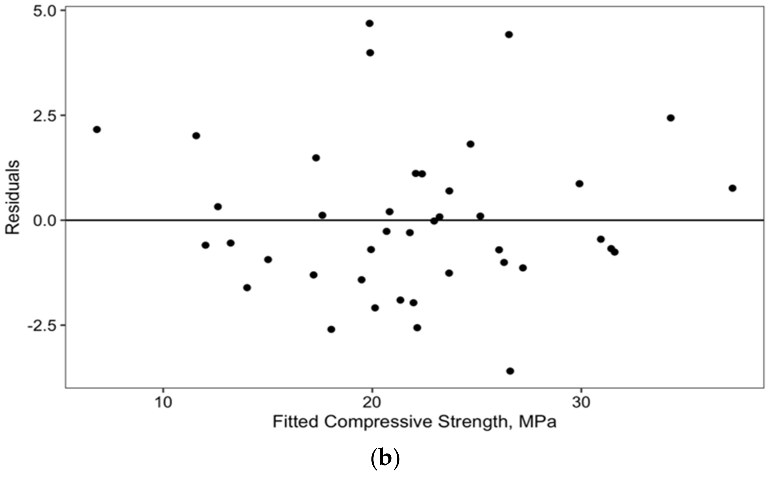
Figure 5 presents a comparison between observed and predicted compressive strength values from Equation (8) using the data from the mixtures included in this study. Overall, there is very good agreement between observed and predicted strength values (R² = 0.93), and most of the values are within the 95% prediction interval. Finally, it can be observed in Figure 5a that the hypothesis of the randomness of residuals holds. It should be noted that in some cases, larger deviations from the equality between observed and predicted values are encountered. Figure 5a thus reflects sources of variability, such as sample to sample variations of the same concrete mix, testing accuracy, temperature control, and experimental-related factors. Thus, “master curves” represent mathematical expressions of experimental data, and any uncertainty in the testing process could cause some variation between experimental and predicted data.

Finally, since relationships between static and dynamic moduli have been developed and proposed in the literature for various mixtures, these can be used to estimate the elastic parameters from destructive testing. However, if the concrete mixtures of interest are not represented in the data used to develop such relationships, these must be further validated.

Since, as mentioned on several occasions, “maturity” is mixture-specific, calibration of any model with data from other mixtures of interest is necessary. Since the objective of this study was to propose an NDT-based maturity approach for the specific and/or typical concrete mixtures encountered in infrastructure project in the region, validation of such models beyond these concretes was beyond the scope of the study. For such cases, validation will require expanding the study to include materials and proportioning for the additional concrete mixtures of interest.

4. Discussion

The analysis and findings of this study indicated that the novel approach of establishing “master curves” in maturity modeling proposed by this research for the first time is feasible and with excellent results. The selected NDTs included in the study can be successfully used in concrete maturity. Since the relationship between concrete quality measures (e.g., compressive strength, UPV, or modulus of elasticity from RFT) and maturity index are mixture-specific, this study explored the development of a representative maturity function, identified herein as a “master curve.” The analysis indicated that NDT-based maturity models provided good fit and were of the same model form (i.e., logarithmic). Specifically:

• The best fit model relating NDT response and the maturity temperature–time product is of logarithmic form, providing a coefficient of determination in almost all cases above 0.9 and p < 0.05, thus resulting in a very good fit for these two parameters and consistent model form for all concrete mixtures that were included in this study.

This led to the development of a “master curve” for maturity. The methodology for defining the shift for each mixture maturity curve to the generalized form (i.e., master curve) was obtained through the definition of a transfer function in relation to key concrete properties, according to the following:

• The “master curve” shift factors were successfully related to concrete mixture properties. These properties were selected based on Pearson’s correlation analysis. Based on alternative model fitting, this led to the inclusion of compressive strength, air content, and average concrete temperature for ${\mathsf{\delta }}_{\mathrm{U}\mathrm{P}\mathrm{V}}$ and compressive strength, unit weight, and average concrete temperature for ${\mathsf{\delta }}_{\mathrm{D}\mathrm{M}}$, respectively. In terms of prediction accuracy, as it was observed from the results, the prediction accuracies for the selected models were 91% and 94% for the UPV and the dynamic modulus shift factor cases (Table 6 and Table 7).
• The shift factor equations were successfully defined using linear regression multivariate analysis, and the “master curves” for pulse velocity and dynamic modulus were defined providing an excellent fit (R² = 1, Figure 3).

A compressive strength prediction model was successfully developed in relation to the maturity index and NDT response, providing a high coefficient of determination (R² = 0.93, Equation (8)). In terms of prediction accuracy, Figure 5a presents a comparison between observed and predicted compressive strength values from Equation (8) using the data from the mixtures included in this study. Overall, there is very good agreement between observed and predicted strength values, and most of them are within the 95% prediction interval.

In terms of limitations of the study findings, since MI is mixture-specific, the applicability of this modeling works well for a group of concrete mixtures in which similar ingredients and compositions are used. This reflects the fact that chemistry kinetics during hydration follow similar trends. In fact, this research has proven that when mixtures of similar content and ingredients are used, the “master curves” concept in maturity works very well. Thus, the development of “master curves” for different types of concretes (such as self-consolidating and fiber-reinforced concrete or when use of alternative cementitious materials like fly ash and slag cements are used) should be further validated since chemistry kinetics may be significantly altered.

5. Summary and Conclusions

Use of NDTs in assessing concrete quality during production and/or construction may provide significant benefits, including faster results in relation to destructive testing and increases in testing frequency without significant increase in cost. This study explored the use of well accepted NDTs for modeling concrete maturity. The results indicated that such NDTs can be successfully used in concrete maturity, and that NDT-based maturity models provided good fit, and, of the same model form (i.e., logarithmic). In terms of scientific novelty, this led to the definition and development of “master curve” maturity modeling for the first time. Furthermore, the methodology for defining the shift for each mixture maturity curve to the generalized form (i.e., master curve) was successfully obtained through the definition of a transfer function in relation to key concrete properties. From the practical point of view, the benefits of developing universal master curve functions for concretes of different types include predicting strength without having to repeat maturity testing each time a producer adjusts mixture proportioning to fine tune mix design, being able to quickly predict what will be the strength gain for variations in mixture proportioning and field curing conditions, and saving time and testing cost by reducing maturity testing.

In terms of concrete strength predictions, while the objective of this study was not to compare models proposed from past studies, a subset of these were considered for assessing the best model form (i.e., non-linearity) between compressive strength and pulse velocity. Recognizing that some of these models were also developed for specialized concrete mixtures, as indicated in the analysis, their prediction accuracy with the data of this study was inferior to those developed herein, for which very good agreement between observed and predicted strength values (R² = 0.93) was observed and for which most of the values were within the 95% prediction interval.