Design and Mechanical Properties of Negative Poisson’s Ratio Structure-Based Topology Optimization

Abstract

Scholars have shown significant interest in the design and investigation of mechanical metamaterials with a negative Poisson’s ratio as a result of the rapid progress in additive manufacturing technology, giving rise to the concept of metamaterials. The mechanical properties of structures with a negative Poisson’s ratio, including Poisson’s ratio, elastic modulus, and impact performance, have received growing scrutiny. This paper introduces the design of a novel concave beetle-shaped structure with a negative Poisson’s ratio. The structure is developed using the variable density topology optimization method, with the design parameters adjusted to achieve optimal results from six datasets. The mechanical properties of the concave beetle-shaped structure are comprehensively assessed with the integration of mathematical models derived from mechanics theory, quasi-static compression tests, and finite element analyses. This study’s findings indicate that the intrinsic parameters of the structure significantly influence its properties. The structure’s Poisson’s ratio ranges from −0.267 to −0.751, the elastic modulus varies between 1.078 and 5.481 MPa, and the specific energy absorption ranges from 1.873 to 2.634 kJ/kg, demonstrating an improvement of up to 40%.

1. Introduction

The mechanical properties of materials have been a primary area of practical application and extensive study. Nevertheless, many material designs remain theoretical as they are not producible or experimentally verifiable due to manufacturing process limitations. However, the advent of additive manufacturing and machine learning design technologies has presented a practical manufacturing method for modern material design. Additive manufacturing technology offers greater freedom for material design with its superior mechanical properties and high precision compared to traditional machining processes like turning, milling, casting, forging, and welding. Consequently, the concept of metamaterials has emerged.

The term “metamaterials” derives from the prefix “meta” meaning “beyond”, implying that the properties or structure of these materials surpass those of traditional materials. The introduction of this terminology originated from a paper published by Smith et al. [1], which investigated a material with negative permeability and dielectric constant at microwave frequencies. Progressively, researchers gained a better understanding of the metamaterial concept. In essence, metamaterials are composite materials and artificial composite structures designed and created with specific parameters, mimicking the attributes and properties of natural materials. The resulting material exceeds the abilities of the natural ones that make it up, and its macroscopic characteristics are largely determined by the microstructure of the material. Barchiesi et al.’s [2] work focused on the evolution and advancement of metamaterials, including their connections with emerging technology. Consequently, they showed that human thought plays a pivotal role in constructing new theories, as stated by Carnap’s [3] deductive and falsificationist methods in the early 20th century.

In recent years, metamaterials research has rapidly progressed across various disciplines, including fundamental physics, optics, materials science, mechanics, and electrical engineering. Metamaterials research is roughly categorized into extraordinary electromagnetic materials [4], optical metamaterials [5,6,7], acoustic metamaterials [8,9], thermal metamaterials [10], and mechanical metamaterials. Yu et al.’s [11] taxonomy classified mechanical metamaterials into four types: (1) strong lightweight materials concerning Young’s modulus, (2) tunable stiffness materials concerning shear modulus, (3) negative compressibility materials concerning bulk modulus, and (4) negative Poisson’s ratio materials concerning Poisson’s ratio.

In recent years, the study of mechanical metamaterial structures has led to significant interest among researchers in negative Poisson’s ratio materials. Regarding the structure of negative Poisson’s ratio materials, researchers have conducted a lot of theoretical and applied research [12,13]. The analysis of negative Poisson’s ratio materials can be approached from the following aspects.

Kolpakov [14] was the first to propose an approximate calculation method to determine the average elastic properties of periodic unit cell framework structures, and he discovered the construction of a framework that has negative Poisson’s ratio properties. Evans [15] named materials with a negative Poisson’s ratio effect as “auxetic materials”. Negative Poisson’s ratio materials have higher stiffness, strength, energy absorption, and damage resistance than materials with a positive Poisson’s ratio [16]. Some complex porous structures made up of ligaments with complex shapes and density gradients have higher structural efficiency than some traditional materials. For example, a comparison can be drawn between the pyramid complex in Giza, Egypt, and the Eiffel Tower in Paris. Even though the structure of the Eiffel Tower is similar to that of the pyramid complex, it has twice the height and is three orders of magnitude lighter in weight [17].

The first thermodynamically stable model with an isotropic phase of the negative Poisson’s ratio was studied using Monte Carlo simulations in Wojciechowski [18]. It was shown that depending on the density or molecular anisotropy, the model can show any negative value of the Poisson’s ratio allowed for isotropic systems [19]. Hoover et al. [20], using computer simulations, investigated auxetic properties on the mezoscopic level. The first isotropic chiral structures were those proposed by Wojciechowski [21]. Later, many scholars simplified and analyzed these structures [22,23,24]. Tretiakov [25] and Narojczyk et al. [26] provided ideas for the design of negative Poisson’s ratio structures in the microscopic domain. Czarnecki et al. [27,28] reported certain innovations in the optimization method. It is also important to stress that some apparently auxetic structures can show completely nonauxetic properties [29,30,31].

Structures with a negative Poisson’s ratio can be designed using two approaches: intuition and creativity and precise mathematical and mechanical calculations using topology optimization. While most proposed mechanical metamaterials are designed empirically, topology optimization has become a more suitable method for mechanical design.

In the field of topology optimization, different approaches to topology optimization are emphasized in different domains. With the expansion of application areas, an increasing number of theories and methods have been introduced. Bendsøe et al. [32] proposed the simplified isotropic material with penalization (SIMP) method, which introduces a hypothetical variable density as a design variable acting on the physical parameters of the material (such as the elastic modulus). By changing the density ρ of the structure’s elements, the topology of the structure can be altered. Xie et al. [33], building upon the previous evolutionary structural optimization (ESO) method, introduced a more mature method called bi-directional evolutionary optimization (BESO). This method is often used for optimization problems such as minimizing displacement, and it does not require sensitivity analyses. Da et al. [34] proposed the evolutionary topology optimization (ETO) algorithm, which can generate clear and smooth boundaries. Additionally, the resulting designs are less dependent on the initial guessed design and finite element mesh resolution. Fu et al. [35] introduced a novel smooth continuum topology optimization algorithm called smooth-edged material distribution for optimizing topology (SEMDOT). This algorithm was shown to obtain designs with smooth and clear boundaries, and it is characterized by its ease of use, flexibility, and high efficiency. Hang [36] presented a floating projection topology optimization (FPTO) method, which is used to seek smooth designs using alternative material models or 0/1 designs using material penalization models.

Lakes [37] introduced an isotropic negative Poisson’s ratio foam structure that was derived from traditional low-density open-cell polymer foam. This foam structure exhibited enhanced elasticity compared to conventional foams. The study provided insights into the design of novel re-entrant foams as a precursor to future developments in negative Poisson’s ratio materials. Xia et al. [38] utilized a MATLAB-based, energy-based homogenization method to optimize the topology of negative Poisson’s ratio materials. Their optimization targets included the bulk modulus, shear modulus, and Poisson’s ratio. Similarly, Lee et al. [39] introduced a topology optimization approach that used Gaussian point density as a design variable. This method served as a basis for developing materials with a negative Poisson’s ratio and showcased the efficacy of topology optimization tools in analyzing such materials. Chen et al. [40] combined negative and positive Poisson’s ratio topologies to achieve an effective zero Poisson’s ratio topology, demonstrating the unique performance of each and providing valuable data for the design of novel structures. Chatterjee [41] used bidirectional evolutionary topology optimization and energy-based homogenization methods to show how material uncertainty can affect the optimal microstructure of mechanical metamaterials, highlighting the importance of considering uncertainty in topology optimization for the mechanical performance and robustness of metamaterials.

This study uses a variable density topology optimization algorithm to design a beetle-inspired concave structure by adjusting the material distribution factor. The designed structure is then manufactured using 3D printing. The effective elastic modulus and Poisson’s ratio are explored using mechanical theory, and the mechanism associated with the structure’s energy absorption is analyzed by examining various structural parameters using simulation results.

2. Design of a Negative Poisson’s Ratio Structure Based on the Variable Density Method

This section seeks negative Poisson’s ratio structures using topology optimization. The widely used methods include homogenization, variable density, level set, and progressive methods. The SIMP method is widely used in finite element software programs. It offers several advantages in microstructure design. Therefore, it is selected as the method for this study. The basic idea of this method is to use the density of each element as a design variable, calculate the effective material parameters corresponding to the density value using the homogenization method, and obtain the optimal distribution of materials throughout the structure using iteration [42,43].

2.1. Objective Function

Assuming the relationship between stress and strain is:

$${\sigma }_{ij}=C_{ijkl}{\epsilon }_{kl}$$

(1)

where the expression of $C_{ijkl}$ for the homogenized elastic tensor is:

$$C_{ijkl}^H=\frac{1}{\left|Y\right|}{\displaystyle \underset{Y}{\int }{C}_{ijpq}({\epsilon }_{pq}^{0(kl)}-{\epsilon }_{pq}^{\mathrm{*}(kl)})}dY$$

(2)

where $Y$ is the base cell domain, $C_{ijpq}$ is the elasticity tensor in index notation, ${\epsilon }_{pq}^{0(kl)}$ is the unit test strain fields, and ${\epsilon }_{pq}^{\mathrm{*}(kl)}$ is the periodic fluctuation strain fields.

According to Sigmund’s [44] proposed theory of element interconnectivity, further calculations for topology optimization are facilitated. The Formula (2) is rewritten as follows:

$$Q_{ijkl}^H=\frac{1}{\left|Y\right|}{\displaystyle \sum _{e=1}^N{({\mathrm{u}}_e^{A(ij)})}^T{k}_e{\mathrm{u}}_e^{A(kl)}}$$

(3)

where N is the number of elements obtained by dividing the entire design domain into N parts, ${\mathrm{u}}_e^{A(ij)}$ is the element displacement vector for load case ij, and $k_e$ is the stiffness.

The objective of topology optimization in this paper is to design a suitable structure in a two-dimensional plane and then finally convert $Q_{ijkl}^H$ into $Q_{ij}^H$ in a two-dimensional problem. To do this, we rewrite Equation (4) in extended form, as shown below:

$$\left[\begin{array}{ccc}{C}_{11}^H& C_{12}^H& C_{13}^H\\ C_{21}^H& C_{22}^H& C_{23}^H\\ C_{31}^H& C_{32}^H& C_{33}^H\end{array}\right]=\left[\begin{array}{ccc}{Q}_{11}& Q_{12}& Q_{13}\\ Q_{21}& Q_{22}& Q_{23}\\ Q_{31}& Q_{32}& Q_{33}\end{array}\right]$$

(4)

where $C_{11}^H$ and $C_{22}^H$ are the theoretical equivalent moduli of elasticity in directions 1 and 2, respectively, $Q_{11}$ and $Q_{22}$ are the principal strain energies in directions 1 and 2, respectively, and $E_{12}^H$ and $C_{12}$ are theoretical shear modulus and the shear strain energy, respectively.

$$Q_{ij}=\frac{1}{\left|Y\right|}{\displaystyle \sum _{e=1}^N{q}_e^{(ij)}}$$

(5)

$$q_e^{(ij)}={({\mathrm{u}}_e^{A(i)})}^T{k}_e{\mathrm{u}}_e^{A(j)}$$

(6)

where $q_e^{(ij)}$ is the element e mutual energy, ${\mathrm{u}}_e^{A(i)}$ is the element displacement vector for load case ij, and $k_e$ is the element stiffness matrix.

The method uses Young’s modulus based on the pseudo-density of the element.

$$E_e(x_e)=E_{min}+x_e^p(E_0-E_{min}),\hspace{1em}{x}_e\in [0,1]$$

(7)

In the equation, $E_e$ is the Young’s modulus of the final material, $E_{min}$ is the Young’s modulus of the substitute material, and $E_0$ is the Young’s modulus of the starting material.

Directly using the Poisson’s ratio formula -C₁₂/C₁₁ as the objective function and the existing optimization criteria for iterative optimization can be highly challenging. However, based on the formulation proposed by Xia [38], topology optimization introduces different relaxation factors into two-dimensional problems. This approach enables the optimized topology structure to maintain a negative Poisson’s ratio while significantly improving the unidirectional stiffness of the resulting microstructure unit cells.

The mathematical expression of the objective function in the final optimization problem is:

$$\begin{array}{l}\min \mathrm{:}c=C_{12}-[{(0.8-\beta )}^l·C_{11}+{0.8}^l·C_{22}]\\ \mathrm{Subject} \mathrm{to}:{\mathrm{KU}}^{A(kl)}=F^{(kl)},k,l=1,\dots ,d\\ \hspace{1em}\hspace{1em}\hspace{1em}\hspace{1em} {\displaystyle \sum _{e=1}^N{\upsilon }_e{x}_e\le V}\\ \hspace{1em}\hspace{1em}\hspace{1em}\hspace{1em} 0\le x_e\le 1,e=1,\dots ,N\end{array}$$

(8)

where $c$ is the objective function, $l$ is the number of iterations, $\mathrm{K}$ is the sparse matrix of the total stiffness of the structure, $F$ and $\mathrm{U}$ are the force vector and displacement vector of the structure, respectively, ${\upsilon }_e$ is the volume of the e-th element, $V$ is the volume constraint after optimization, which is the product of the volume fraction and the original volume, and $x_e$ is the design variable, that is, the relative density of each element.

To ensure continuity in the derivation, when both geometric shapes and loads exhibit symmetry, it is possible to apply them directly without converting them into traditional boundary conditions. This type of boundary condition is referred to as a periodic boundary condition (PBC). Such a boundary condition can be directly imposed on a finite element model using constrained nodal displacements, while also satisfying the periodicity and continuity requirements of both displacement and stress.

2.2. Sensitivity Calculation

Throughout optimization, the degree to which a cell is retained or deleted is determined by the sensitivity of that element. In topology optimization, sensitivity describes how strongly a design variable affects the optimization objective. By identifying the design variables with the strongest influence on the optimization objective, the algorithm can find the direction toward the optimal solution.

The direct differentiation method is used to solve the sensitivity by differentiating the objective function with respect to the design variables. The sensitivity of the objective function to the design variables can be expressed as:

$$\frac{\partial c}{\partial x_e}=\frac{\partial C_{12}}{\partial x_e}-[{(0.8-\beta )}^l·\frac{\partial C_{11}}{\partial x_e}+{0.8}^l·\frac{\partial C_{22}}{\partial x_e}]$$

(9)

The following expression can be obtained by combining Equations (7) and (9):

$$\frac{\partial c}{\partial x_e}=p{x}_{{}^e}^{p-1}(E_0-E_{min})·q{e}^{12}-[{(0.8-\beta )}^l·p{x}_e^{p-1}(E_0-E_{min})·q{e}^{11}+{0.8}^l·p{x}_e^{p-1}(E_0-E_{min})·q{e}^{22}]$$

(10)

Substituting Equation (6) into Equation (10) gives:

$$\frac{\partial c}{\partial x_e}=p{x}_e^{p-1}(E_0-E_{min})·[{({\mathrm{u}}_e^{A(1)})}^T{k}_e{\mathrm{u}}_e^{A(2)}]-\left\{\begin{array}{l}{(0.8-\beta )}^l·p{x}_e^{p-1}(E_0-E_{min})·[{({\mathrm{u}}_e^{A(1)})}^T{k}_e{\mathrm{u}}_e^{A(1)}]+\\ {0.8}^l·p{x}_e^{p-1}(E_0-E_{min})·[{({\mathrm{u}}_e^{A(2)})}^T{k}_e{\mathrm{u}}_e^{A(2)}]\end{array}\right\}$$

(11)

According to Equation (11), it can be found that the number of iterations $l$, penalty factor $p$, Young’s modulus $E_0$, and $E_{min}$, relaxation factor $\beta$ will all have an impact on the optimization of the objective function.

2.3. Optimization Examples and Analysis

The example in Figure 1 uses N_x and N_y to represent the number of elements in the x and y directions of the initial structure, respectively. The volume fraction is defined as the percentage of the optimized structure’s volume to the initial volume. For example, if volfrac = 0.5, the volume of the optimized structure is 50% of the initial volume. The variable density method requires a penalty factor, which penalizes intermediate density units to minimize the number of density units and make the density tend toward 0 or 1. An appropriate penalty factor is crucial since a small penalty factor creates many gaps that make material manufacturing difficult, while large penalty factors increase optimization iterations and time costs. The filtering radius affects the material density distribution and stability of optimization results. A larger filtering radius increases smoothness at the expense of the accuracy and details of the optimization results, creating refinement and instability. Choosing the right optimization parameters is, therefore, crucial. There are two types of filtering options: density filtering and sensitivity filtering. Density filtering involves modifying the sensitivity information of the objective function and volume constraints to obtain pseudo-densities for each element. On the other hand, sensitivity filtering directly filters the sensitivity information of the objective function using the design variables, which represent the pseudo-densities of the elements. During topological optimization, the interior of the structure is set as a “blank area” to maintain material connectivity and ensure physical feasibility. Material density in these blank areas is relatively low.

N_x and N_y determine the initial size of the structure but have minimal influence on the optimized structure. The volume fraction and blank region radius directly impact the morphology of the optimized structure. Therefore, fixed values are chosen for the penalty factor and filtering radius due to their widespread applicability. Different filtering methods have a significant impact on both the structure and the objective function, so they are chosen as parameters to be varied. Taking into account the effects of these parameters, six sets of data in

Table 1. Specific parameters for six sets of topology optimization data.

Group	N_x	N_y	Volume Fraction	Penalty Factor	Filtering Radius	Filter Type	Radius of the Blank Area
A	100	100	0.5	3	5	density filtering	16.7
B	100	100	0.4	3	5	density filtering	16.7
C	100	100	0.3	3	5	density filtering	16.7
D	100	100	0.5	3	5	sensitivity filtering	16.7
E	100	100	0.5	3	5	sensitivity filtering	20
F	100	100	0.5	3	5	sensitivity filtering	10

are selected for MATLAB programming to implement the topology optimization algorithm. The final values of the objective function are compared to determine the most suitable parameters.

Figure 2 presents the numerical variation charts for the objective function obtained by comparing the six sets of data. The charts show that the value of the objective function rapidly decreases as the number of iterations increases and then stabilizes at a converged value. However, groups E and F exhibit oscillations between two objective function values, which may be due to the optimization algorithm being trapped in a local minimum. Sensitivity filtering smooths the objective function during the optimization process, but changing the initial value or parameters is necessary to achieve convergence. To improve the optimization results, the value of β will be changed in the next step of this article to achieve optimal convergence.

The final objective function value can be affected by the volume fraction, filtering method, and size of the blank region, while the number of basic units remains constant. By comparing groups A, B, and C, it was observed that smaller volume fractions resulted in larger objective function values. Moreover, using sensitivity filtering reduced the objective function value, as noted with the comparison between groups A and D. Additionally, the radius of the blank region affects the objective function value, although the impact is irregular, and an optimal blank region size must be identified. Given these observations, this article selects data sets A, D, and E to study the impact of the relaxation factor β on the objective function by changing its value.

The unit cell configurations for group A under different β values are shown in

Table 2. Variation in the objective function and Poisson’s ratio for group A data under different β.

Group A	Objective Function	C12	C11	C12/C11
β = 0	−0.034	−0.034	0.0762	−0.446
β = 0.002	−0.0326	−0.0325	0.0736	−0.442
β = 0.004	−0.0297	−0.0297	0.0486	−0.611
β = 0.006	0	3.3 × 10−10	1.1 × 10−9	0.3

and Figure 3.

The unit cell configurations for group D under different β values are shown in

Table 3. Variation in the objective function and Poisson’s ratio for group D data under different β.

Group D	Objective Function	C12	C11	C12/C11
β = 0	−0.0399	−0.0399	0.1233	−0.324
β = 0.004	−0.0558	−0.0545	0.0754	−0.723
β = 0.008	−0.0453	−0.0451	0.0943	−0.478
β = 0.010	−0.0484	−0.0489	0.0672	−0.728
β = 0.012	0	1.36 × 10−09	4.61×10−09	0.295

and Figure 4.

The unit cell configurations of group E under different β values are shown in

Table 4. Variation in the objective function and Poisson’s ratio for group E data under different β.

Group E	Objective Function	C12	C11	C12/C11
β = 0	−0.0327	−0.0327	0.105	−0.311
β = 0.005	−0.0754	−0.0754	0.135	−0.557
β = 0.010	−0.0755	−0.0755	0.140	−0.539
β = 0.020	−0.0760	−0.0760	0.0133	−0.572
β = 0.030	0	9.6 × 10−10	3.29 × 10−10	0.292

and Figure 5.

In the tables, the values for C₁₂ and C₁₁ represent the theoretical equivalent elastic modulus. Poisson’s ratio is calculated using the formula C₁₂/C₁₁. Notably, Poisson’s ratio is defined within the range of −1 to 0.5 within the elastic regime. It should be stressed that in two dimensions, the Poisson’s ratio for isotropic media can vary between −1 and +1 [21]. For anisotropic systems, PR may take an even broader range of values.

From the above data analysis, significant changes in the value of the objective function occur when β = 0 and β = 0.002 for Group D, as well as when β = 0 and β = 0.005 for Group E. When the β values in Groups A, D, and E are too large, the corresponding objective functions are all zero. As β increases, the material in the x-direction decreases, while the material in the y-direction increases. From this observation, it is affirmed that the relaxation factor β could influence the design of negative Poisson’s ratio structures. When the β value in Group A exceeds 0.004, the β value in Group B exceeds 0.010, and the β value in Group C exceeds 0.020, the decrease in the material in the x-direction is extensive, resulting in over-optimization and the emergence of a vertical beam. At this point, the Poisson’s ratio of the beam is akin to the Poisson’s ratio set as a basic material value of 0.3.

The optimal selection for basic values of topology optimization involves a relaxation factor β = 0.02, as obtained from group E. The selection comprises 100 x elements, 100 y elements, a volume fraction of 0.5, a penalty factor of 3, a filter radius of 5, density filtering, a blank radius of 20, and a relaxation factor β = 0.02. The final expression for topology optimization is as follows:

$$\begin{array}{l}\mathrm{m}\mathrm{i}\mathrm{n}:c=C_{12}-[{0.78}^l·C_{11}+{0.8}^l·C_{22}]\\ \mathrm{S}\mathrm{u}\mathrm{b}\mathrm{j}\mathrm{e}\mathrm{c}\mathrm{t} \mathrm{to}:\mathrm{K}{\mathrm{U}}^{A(kl)}=F^{(kl)},k,l=1,\dots ,d\\ \hspace{1em}\hspace{1em}\hspace{1em}\hspace{1em} {\displaystyle \sum _{e=1}^N{\upsilon }_e{x}_e\le V}\\ \hspace{1em}\hspace{1em}\hspace{1em}\hspace{1em} 0\le x_e\le 1,x=1,\dots ,N\end{array}$$

(12)

The objective function and Poisson’s ratio variation during the topology optimization process are shown in Figure 6 and Figure 7, respectively.

3. Structural Geometric Construction and Equivalent Elastic Properties

The variable density method enabled topology optimization to design a negative Poisson’s ratio cell structure. To investigate its mechanical properties accurately, a suitable geometric structure was extracted for modeling, as illustrated in Figure 8. In this figure, the transverse edge of the unit cell is represented by 2a, and the vertical edge of the unit cell is 2h. Meanwhile, the oblique edge of the unit cell is denoted with b, and the concave edge is represented with c. Additionally, the length of the connecting rod that joins the horizontal cells is called p. The acute angle between the oblique edge and the transverse edge is denoted with α, while the acute angle between the concave edge and the connecting rod is denoted with γ.

This paper sets the thickness at 0.65 mm and connecting rod thickness at 5 mm, taking into account the accuracy issues associated with finite element analysis and 3D printing. The focus of this paper is to investigate the influence of transverse edge a, oblique edge b, concave edge c, vertical edge h, and two angles α and γ on the equivalent elastic modulus and Poisson’s ratio. Furthermore, due to cellular connection problems, geometric parameters are subjected to constraints imposed using Equation (13) to ensure the rationality and coordination of the overall structure.

$$c·\cos \gamma <a+b·\cos \alpha$$

(13)

3.1. Theoretical Calculation

The corner deformation compatibility condition at free end D satisfies:

$${\delta }_{11}{M}_0+{\delta }_{1F}=0$$

(14)

In the given formula, ${\delta }_{1F}$ represents the angle of rotation at point D when it is solely subjected to the load F/2 and ${\delta }_{11}$ denotes the angle of rotation at point D when it is subjected to a unit moment specifically applied at point D.

As shown in Figure 9c, the bending moments of segments AB, BC, and CD can be calculated when only subjected to F/2. As shown in Figure 9d, when only subjected to a unit moment, the bending moments of each segment can be obtained. Using Mohr’s theorem [45] to perform Mohr integral for each beam, ${\delta }_{1F}$ and ${\delta }_{11}$ can be respectively determined:

$$\begin{array}{lll}{M}_{AB}\left(x_1\right)=\frac{F}{2}(\mathrm{b}\mathrm{c}\mathrm{o}\mathrm{s}\alpha -\mathrm{c}\mathrm{c}\mathrm{o}\mathrm{s}\beta )+\frac{F}{2}{x}_1& x_1\in \left(0,\mathrm{a}\right)& \overline{M_{AB}}\left(x_1\right)=-1;\end{array}$$

(15)

$$\begin{array}{lll}{M}_{BC}\left(x_2\right)=-\frac{F}{2}c\cos \beta +\frac{F}{2}{x}_2\cos \alpha \hspace{1em} & x_2\in \left(0,\mathrm{b}\right)& \overline{M_{BC}}\left(x_2\right)=-1;\end{array}$$

(16)

$$\begin{array}{lll}{M}_{CD}\left(x_3\right)=-\frac{F}{2}{x}_3\cos \beta \hspace{1em}\hspace{1em}\hspace{1em}\hspace{1em}\hspace{1em}\hfill & x_3\in \left(0,\mathrm{c}\right)& \overline{M_{BC}}\left(x_3\right)=-1;\end{array}$$

(17)

$${\delta }_{1F}={\displaystyle {\int }_0^a\frac{M_{AB}\left(x_1\right)\overline{M_{AB}}\left(x_1\right)}{E_m{I}_m}}d{x}_1+{\displaystyle {\int }_0^b\frac{M_{BC}\left(x_2\right)\overline{M_{BC}}\left(x_2\right)}{E_m{I}_m}}d{x}_2+{\displaystyle {\int }_0^c\frac{M_{CD}\left(x_3\right)\overline{M_{CD}}\left(x_3\right)}{E_m{I}_m}}d{x}_3$$

(18)

$${\delta }_{11}={\displaystyle {\int }_0^a\frac{\overline{M_{AB}}\left(x_1\right)\overline{M_{AB}}\left(x_1\right)}{E_m{I}_m}}d{x}_1+{\displaystyle {\int }_0^b\frac{\overline{M_{BC}}\left(x_2\right)\overline{M_{BC}}\left(x_2\right)}{E_m{I}_m}}d{x}_2+{\displaystyle {\int }_0^c\frac{\overline{M_{CD}}\left(x_3\right)\overline{M_{CD}}\left(x_3\right)}{E_m{I}_m}}d{x}_3$$

(19)

In Equations (18) and (19), $E_{\mathrm{m}}$ represents the elastic modulus of the material and $I_{\mathrm{m}}$ represents the moment of inertia of the cross-section with respect to the neutral axis. From Equations (18) and (19), it follows that:

$$M_0=-\frac{{\delta }_{1F}}{{\delta }_{11}}=\frac{F}{4}\left(\frac{a^2+b^2\cos \alpha -c^2\cos \beta +2ab\cos \alpha -2ac\cos \beta -2bc\cos \beta }{a+b+c}\right)=F\theta$$

(20)

where $\theta =\frac{1}{4}\left(\frac{a^2+b^2\cos \alpha -c^2\cos \beta +2ab\cos \alpha -2ac\cos \beta -2bc\cos \beta }{a+b+c}\right)$.

According to Castigliano’s theorem [46], the displacement deformation of each segment in the y-axis direction can be calculated under the symmetric load of F/2 in the y-axis direction:

$$\begin{array}{ll}{M}_{AB}\left(x_1\right)=\frac{F}{2}(\mathrm{b}\mathrm{c}\mathrm{o}\mathrm{s}\alpha -\mathrm{c}\mathrm{c}\mathrm{o}\mathrm{s}\beta )+\frac{F}{2}{x}_1-M_0& x_1\in \left(0,\mathrm{a}\right)\\ \overline{M_{AB}}\left(x_1\right)=(\mathrm{b}\mathrm{c}\mathrm{o}\mathrm{s}\alpha -\mathrm{c}\mathrm{c}\mathrm{o}\mathrm{s}\beta )+x_1-2\theta ;\end{array}$$

(21)

$$\begin{array}{ll}{M}_{BC}\left(x_2\right)=-\frac{F}{2}\mathrm{c}\mathrm{c}\mathrm{o}\mathrm{s}\beta +\frac{F}{2}{x}_2\cos \alpha -M_0& \hspace{1em}{x}_2\in \left(0,\mathrm{b}\right)\\ \overline{M_{BC}}\left(x_2\right)=-\mathrm{c}\mathrm{c}\mathrm{o}\mathrm{s}\beta +x_2\cos \alpha -2\theta ;\end{array}$$

(22)

$$\begin{array}{ll}{M}_{CD}\left(x_3\right)=-\frac{F}{2}{x}_3\cos \beta -M_0& \hspace{1em}\hspace{1em}\hspace{1em}\hspace{1em}{x}_3\in \left(0,\mathrm{c}\right)\\ \overline{M_{CD}}\left(x_3\right)=-x_3\cos \beta -2\theta ;\end{array}$$

(23)

$${∆}_{YY}=\frac{2}{E_m{I}_m}\left[{\displaystyle {\int }_0^a{M}_{AB}\left(x_1\right)\overline{M_{AB}}\left(x_1\right)}d{x}_1+{\displaystyle {\int }_0^b{M}_{BC}\left(x_2\right)\overline{M_{BC}}\left(x_2\right)}d{x}_2+{\displaystyle {\int }_0^c{M}_{CD}\left(x_3\right)\overline{M_{CD}}\left(x_3\right)}d{x}_3\right]$$

(24)

$${∆}_{YY}=\frac{F}{3E_m{I}_m}\left[\begin{array}{l}3a{(\mathrm{b}\mathrm{c}\mathrm{o}\mathrm{s}\alpha -\mathrm{c}\mathrm{c}\mathrm{o}\mathrm{s}\beta )}^2+3a^2(\mathrm{b}\mathrm{c}\mathrm{o}\mathrm{s}\alpha -\mathrm{c}\mathrm{c}\mathrm{o}\mathrm{s}\beta )+a^3-12a\theta (\mathrm{b}\mathrm{c}\mathrm{o}\mathrm{s}\alpha -\mathrm{c}\mathrm{c}\mathrm{o}\mathrm{s}\beta )-\\ 6a^2\theta +12a{\theta }^2+3c^{2}b{\cos }^2\beta -3c{b}^2\cos \alpha \cos \beta +b^3{\cos }^2\alpha +12bc\theta \cos \beta -\\ 6b^2\theta \cos \alpha +12b{\theta }^2+c^3{\cos }^2\beta +6c^2\theta \cos \beta +12c{\theta }^2\end{array}\right]$$

(25)

As shown in Figure 9e, using the unit force method, the displacement deformation of each segment in the x-direction can be calculated under the symmetric load of F/2 in the y-direction:

$$\begin{array}{ll}{M}_{AB}(x_1)=\frac{F}{2}(\mathrm{b}\mathrm{c}\mathrm{o}\mathrm{s}\alpha -\mathrm{c}\mathrm{c}\mathrm{o}\mathrm{s}\beta )+\frac{F}{2}{x}_1-M_0& x_1\in \left(0,\mathrm{a}\right)\\ \overline{M_{AB}}(x_1)=b\sin \alpha +c\sin \beta ;\end{array}$$

(26)

$$\begin{array}{ll}{M}_{BC}(x_2)=-\frac{F}{2}\mathrm{c}\mathrm{c}\mathrm{o}\mathrm{s}\beta +\frac{F}{2}{x}_2\cos \alpha -M_0& \hspace{1em}{x}_2\in \left(0,\mathrm{b}\right)\\ \overline{M_{BC}}(x_2)=c\sin \beta +x_2\mathrm{s}\mathrm{i}\mathrm{n}\alpha ;\end{array}$$

(27)

$$\begin{array}{ll}{M}_{CD}(x_3)=-\frac{F}{2}{x}_3\mathrm{c}\mathrm{o}\mathrm{s}\beta -M_0& \hspace{1em}\hspace{1em}\hspace{1em}\hspace{1em} x_3\in \left(0,\mathrm{c}\right)\\ \overline{M_{CD}}(x_3)=x_3\sin \beta ;\end{array}$$

(28)

$${∆}_{YX}=\frac{2}{E_m{I}_m}\left[{\displaystyle {\int }_0^a{M}_{AB}\left(x_1\right)\overline{M_{AB}}\left(x_1\right)}d{x}_1+{\displaystyle {\int }_0^b{M}_{BC}\left(x_2\right)\overline{M_{BC}}\left(x_2\right)}d{x}_2+{\displaystyle {\int }_0^c{M}_{CD}\left(x_3\right)\overline{M_{CD}}\left(x_3\right)}d{x}_3\right]$$

(29)

$${∆}_{YX}=\frac{F}{6E_m{I}_m}\left[\begin{array}{l}6a(\mathrm{b}\mathrm{c}\mathrm{o}\mathrm{s}\alpha -\mathrm{c}\mathrm{c}\mathrm{o}\mathrm{s}\beta )(\mathrm{b}\mathrm{s}\mathrm{i}\mathrm{n}\alpha +\mathrm{c}\mathrm{s}\mathrm{i}\mathrm{n}\beta )+3{\mathrm{a}}^2(\mathrm{b}\mathrm{s}\mathrm{i}\mathrm{n}\alpha +\mathrm{c}\mathrm{s}\mathrm{i}\mathrm{n}\beta )-12\mathrm{a}\theta (\mathrm{b}\mathrm{s}\mathrm{i}\mathrm{n}\alpha +\mathrm{c}\mathrm{s}\mathrm{i}\mathrm{n}\beta )-\\ 6\mathrm{b}{\mathrm{c}}^2\sin \beta \cos \beta -3b^2\mathrm{c}\sin \alpha \cos \beta +3{\mathrm{b}}^2\mathrm{c}\sin \beta \cos \alpha +2{\mathrm{b}}^3\sin \alpha \cos \alpha -\\ 12\mathrm{b}\mathrm{c}\theta \mathrm{s}\mathrm{i}\mathrm{n}\beta -6{\mathrm{b}}^2\theta \sin \alpha -2{\mathrm{c}}^3\sin \beta \cos \beta -6{\mathrm{c}}^2\theta \sin \beta \end{array}\right]$$

(30)

According to Equations (25) and (30), the numerical values for the stress–strain, equivalent elastic modulus, and equivalent Poisson’s ratio in the y-direction can be obtained. The stress and strain are:

$${\sigma }_y=\frac{F}{2(\mathrm{a}+\mathrm{b}\mathrm{c}\mathrm{o}\mathrm{s}\alpha )z}$$

(31)

$${\epsilon }_{yx}=\frac{{∆}_{YX}}{2(\mathrm{a}+\mathrm{b}\mathrm{c}\mathrm{o}\mathrm{s}\alpha )}$$

(32)

$${\epsilon }_{yy}=\frac{{∆}_{YY}}{2(\mathrm{h}+\mathrm{b}\mathrm{s}\mathrm{i}\mathrm{n}\alpha +\mathrm{c}\mathrm{s}\mathrm{i}\mathrm{n}\beta )}$$

(33)

In the equations, ${\sigma }_y$ represents stress in the y-direction, while ${\epsilon }_{yx}$ and ${\epsilon }_{yy}$ represent strain in the y-direction and x-direction, respectively, when subjected to a force in the y-direction. The equivalent elastic modulus and equivalent Poisson’s ratio are, respectively:

$$E_Y=\frac{{\sigma }_{\mathrm{y}}}{{\epsilon }_{\mathrm{yy}}}=\frac{F}{{∆}_{YY}}\frac{h+b\sin \alpha +c\sin \beta }{(a+b\cos \alpha )z}$$

(34)

$${\nu }_{yx}=-\frac{{\epsilon }_{yx}}{{\epsilon }_{yy}}=-\frac{{∆}_{YX}}{{∆}_{YY}}\frac{h+b\sin \alpha +c\sin \beta }{a+b\cos \alpha }$$

(35)

In the equations, $E_Y$ represents the equivalent elastic modulus when subjected to a load in the y-direction and ${\nu }_{yx}$ represents the equivalent Poisson’s ratio when subjected to a load in the y-direction.

3.2. Comparison of Analytical and Finite Element Results

The commercial finite element software ABAQUS was used to simulate the structure. By changing the parameters that affect the equivalent elastic modulus and Poisson’s ratio of the structure in the theoretical calculations, the influence of geometric parameters on the equivalent elastic modulus and Poisson’s ratio was studied.

The basic parameters of the model are as follows: the transverse edge of the cell is a = 8 mm, the oblique edge is b = 5 mm, the concave edge is c = 5 mm, the vertical edge of the cell is h = 5 mm, the acute angle α between the oblique edge and the transverse edge of the cell is π/4, the acute angle γ between the concave edge and the connecting rod is π/4, and the connecting rod length is p = 5 mm, as shown in Figure 10. The finite element model consisted of a 5 × 5 cell array structure made of aluminum alloy with an elastic modulus of 70 GPa, Poisson’s ratio of 0.33, and density of 2.7 g/cm³. The infrabasal and compression plates were made of steel with an elastic modulus of 207 GPa, Poisson’s ratio of 0.3, and density of 7.8 g/cm³. The number of elements is 118,000; the cell type of the plates is C3D8R, and the number of elements is 90,000; the cell type of the concave beetle-shaped structure is S4R, and the number of elements is 28,000. Displacement from the finite element simulation was used to compute the equivalent elastic modulus and Poisson’s ratio.

3.2.1. The Influence of Various Parameters on the Equivalent Elastic Modulus

The influence of parameters with different ranges was discussed under the condition of restricting other parameters to verify their impact on the equivalent elastic modulus in the analytical solution.

Initially, we investigated the transverse edge length influence on the equivalent elastic modulus of the structure, as depicted in Figure 11a. The structure’s elastic modulus decreases as a increases, as was anticipated. As a increases, the x-direction length of the structure extends, causing the structure to flatten, and the strain decreases, which leads to a decrease in its elastic modulus.

As the length of the oblique edge b increases, Figure 11b demonstrates that the equivalent elastic modulus follows an anticipated pattern of initially decreasing and subsequently reaching a plateau. The structure of the cell can withstand greater force and produce a greater strain as b increases.

As the concave edge c increases, Figure 11c illustrates that the equivalent elastic modulus of the cell structure exhibits an increase, and it is evident that the impact of c’s concave edge on the cell structure’s elastic modulus is significant, making it the primary energy-absorbing component of the cell structure. Although an increase in the lengths of b and c will cause the structure to extend along the y-direction, The influence of the concave edge c on the equivalent elastic modulus of the cell structure is more significant because it is the primary energy-absorbing component.

Figure 11d shows that the vertical edge has an impact on the equivalent elastic modulus of the structure. Increasing the value of h leads to a corresponding increase in the equivalent elastic modulus. Although the increase in h also affects the size of the structure in the y-direction, its influence on the equivalent elastic modulus is more pronounced.

The α and γ angles are both acute angles, and as they increase, the equivalent elastic modulus increases gradually, as shown in Figure 11e. This phenomenon can be explained by the fact that, as the angle of inclination increases when both angles are acute, the primary stress mode of the structure changes. The force on the diagonal rod moves gradually from shear force and bending force to axial force and bending force, contributing to an increase in the equivalent elastic modulus.

3.2.2. The Influence of Various Parameters on the Equivalent Poisson’s Ratio

In order to analyze the influence of various parameters on the equivalent Poisson’s ratio in the analytical solution, we conducted an analysis where we examined the effects of different parameters on the equivalent Poisson’s ratios while keeping the other parameters constant.

To begin with, Figure 12a shows the effect of the transverse edge a on the equivalent Poisson’s ratio. With the gradual increase in a, the equivalent Poisson’s ratio also increases steadily, and the rate of increase is swift, while the negative Poisson’s ratio feature gradually disappears.

The influence of the oblique edge b on the equivalent Poisson’s ratio is the next aspect to consider, as shown in Figure 12b. As b increases, the effective Poisson’s ratio experiences a gradual decrease, displaying negative Poisson’s ratio characteristics, albeit with a moderate reduction rate. It is important to note that while the effective elastic modulus and effective Poisson’s ratio are negatively correlated with other parameters, they exhibit a positive correlation with the oblique edge b.

Parameter c plays a crucial role in the deformation behavior of the structure under substantial forces. In Figure 12c, it is evident that as c increases, the equivalent Poisson’s ratio of the structure gradually decreases, resulting in a more pronounced negative Poisson’s ratio characteristic, aligning with the expected behavior.

Parameter h, which represents the vertical edge of the unit cell, exerts an influence on the equivalent Poisson’s ratio and acts as a moderating factor. This is depicted in Figure 12d.

Parameters α and γ, which represent the angles between edges, significantly impact the trend in the equivalent Poisson’s ratio. Figure 12e demonstrates that the effect of γ is more pronounced. As the angles between the edges increase, the connecting area in the unit cells also increases, resulting in a decrease in the macro-level equivalent Poisson’s ratio. The decrease highlights negative Poisson’s ratio characteristics.

Based on previous experience, the discussion above demonstrates that there is a certain difference between the analytical and simulation solutions that can be categorized into two explanations. Primarily, the energy method used in theoretical derivation neglects the impact of tensile and shear forces, leading to significant disparities between the analytical and simulation solutions for certain results. Additionally, the simulation model used in this paper assumes that all segments are either horizontal or vertical. This assumption may underestimate the impact of forces on some segments during theoretical analysis, leading to underestimated results during segmented integration. Nevertheless, during the simulation process, each segment is capable of undergoing bending deformation as a result of its elasticity, which may cause the simulation solution to exceed the analytical solution in some situations.

4. Crashworthiness Analysis of the Concave Beetle-Shaped Honeycomb Structure

Using the ABAQUS/Explicit solver and the finite element method, this section uses an analysis to examine the relationship between structural parameters and mechanical performance. The focus is on evaluating the impact of different parameters on the energy absorption of the structure, with the original unit cell serving as the reference point.

4.1. Finite Element Model

This section introduces a finite element model consisting of a concave beetle-shaped honeycomb structure sandwiched between two steel plates. The infrabasal plate is immobile, with a unit cell structure measuring 4 × 3 resting atop it. The top plate undergoes a quasi-static compression mode with a fixed downward velocity during the loading process. Both the infrabasal and impacting plates are considered rigid bodies, and the model utilizes steel with a density of 7.8 × 10⁻⁹ t/mm³, an elastic modulus of E = 2.07 × 10⁵ MPa, and a Poisson’s ratio of ν = 0.3. The infrabasal plate is fully constrained, while the impacting plate is limited to movements and rotations along the y-axis.

The concave beetle-shaped honeycomb structure, made of common aluminum metal, possesses a density of ρ = 2.7 × 10⁻⁹ t/mm³, an elastic modulus of E = 7 × 10⁴ MPa, a Poisson’s ratio of ν = 0.33, and a yield stress of 76 MPa. The movements along the x-axis and y-axis and the rotations around the z-axis are the only degrees of freedom permitted. To maintain the accuracy of simulation results and keep computational costs under control, we selected five integration points along the thickness direction of the honeycomb structure while setting the honeycomb structure element mesh size to 0.8 mm and the two-steel plate element mesh size to 1 mm. The number of elements is 118,000; the cell type of the plates is C3D8R, and the number of elements is 90,000; the cell type of the concave beetle-shaped structure is S4R, and the number of elements is 28,000. During the simulation process, we utilized general contact to simulate the frictional interaction between different components of the specimen during the compression process. Refer to Figure 13 for a visual representation of the model.

4.2. Test Validation

A validation test model was fabricated to validate the accuracy of the finite element model. The iSLA880, a light-curing 3D printer from ZRapid Tech, was used to produce the sample with specific material parameters listed in

Table 5. Material properties used in tests and simulations.

Materials	Density (kg/m3)	Young’s Modulus (MPa)	Poisson’s Ratio
Steel	7800	207,000	0.3
Al	2700	70,000	0.33
ZR680 (Resin)	1180	2100	0.35

. The computer-designed 3D CAD file was converted into STL format, which is utilized by most 3D printers to preserve the model’s detailed data. The 3D printer’s system imported the STL file, and specialized software sliced and divided the model. The model was subsequently printed with a 0.1 mm thickness. It is 130 mm in length, 30 mm in width, and 70 mm in height. The Changchun Kexin WDW-300 microcomputer-controlled electronic universal testing machine was utilized for this test, shown in Figure 14, which includes a load mechanism, a driver unit, a load amplifier, testing machine accessories, and other peripheral equipment.

The primary objective of the test is to secure the sample on the infrabasal plate. After starting the motor, the moving beam is driven with a three-stage belt drive to begin the quasi-static compression test at a speed of 2 mm/min. The end condition is when the compression position reaches 40 mm and stops moving. A comparison between the deformation process of the test specimen and the simulation image is shown in Figure 15. It can be seen that as the compression distance increases, the specimen tilts more and more to the left. It is preliminarily judged that the compression speed is too small and the compression distance is too large, which causes the specimen to undergo a “lateral bend”. In subsequent research, it is necessary to consider how to avoid this phenomenon. Finally, the sensor transmits the data of force and displacement to the computer, and the computer integrates the force-displacement curve, as shown in Figure 16. From the figure, we can see that the fitting degree between the simulation solution and the experimental solution is high. The average force for the simulation solution is 693.96 N, and the average force for the experimental solution is 675.64 N, with an error of 2.6%. The error is within an acceptable range, which proves the correctness of the model and finite element simulation and provides a basis and guarantee for further research.

4.3. Influence of Cellular Structural Parameters on Crashworthiness

The variation in parameters in the negative Poisson’s ratio cell structure leads to the change in energy absorption and buffering effects. The structural parameters, such as a, b, c, h, α, and γ, of the original cell were altered to analyze the impact of different cell structure dimensions on the internal energy and specific energy absorption.

4.3.1. The Effect of Cellular Transverse Edge a

The impact performance of the structure based on the transverse edge of the unit cell was analyzed by considering the changes in energy absorption when other structures were left unchanged.

Table 6. Numerical results for specimens with different sizes of a.

a	5	6	7	8	9
b	5	5	5	5	5
c	5	5	5	5	5
h	5	5	5	5	5
α	π/4	π/4	π/4	π/4	π/4
γ	π/4	π/4	π/4	π/4	π/4
Mass (g)	50.1	51.8	53.6	55.3	57.1
Internal energy (mJ)	131,950	130,570	125,853	130,221	126,704
Specific energy absorption (kJ/kg)	2.634	2.521	2.348	2.355	2.21

and Figure 17 present the specific parameters of the cellular structure, as well as internal energy and specific energy absorption under impact. It is evident from Figure 17 that an increase in parameter “a” gradually reduces the specific energy absorption of the structure. Table 6 indicates that increasing “a” leads to an increase in the mass of the entire structure. Hence, the internal energy that the structure bears shows a non-monotonic decreasing trend, in agreement with the specific energy absorption decline in the structure.

4.3.2. The Effect of Cellular Oblique Edge b

The impact performance of the oblique edge of the unit cell was analyzed while keeping the original cell’s other structures unchanged. Changes in energy absorption are scrutinized as the parameter “b” varied from 4 to 6 mm.

The specific parameters of the cellular structure, internal energy, and specific energy absorption curve after the impact are shown in

Table 7. Numerical results for specimens with different sizes of b.

b	4	4.5	5	5.5	6
a	8	8	8	8	8
c	5	5	5	5	5
h	5	5	5	5	5
α	π/4	π/4	π/4	π/4	π/4
γ	π/4	π/4	π/4	π/4	π/4
Mass (g)	52.3	53.8	55.3	56.8	58.3
Internal energy (mJ)	122,969	127,928	130,221	133,175	135,241
Specific energy absorption (kJ/kg)	2.351	2.378	2.355	2.345	2.320

and Figure 18. As the parameter b increases, it leads to an increase in the specific energy absorption. The specific energy absorption reaches its maximum value at b = 4.5 mm and subsequently decreases. Table 7 shows that increasing the parameter “b” increases the mass of the structure, and as a result, the internal energy absorbed by the structure also increases monotonically. However, because of the increase in mass, the specific energy absorption of the structure does not increase monotonically but increases first and then decreases. An analysis of Table 7 concludes that the oblique edge “b” of the unit cell increases the amount of internal energy absorbed by the structure, and thus, it is a crucial factor in determining the energy absorption of the structure. It is recommended to note the b size selection to achieve optimal energy absorption performance.

4.3.3. The Effect of Cellular Concave Edge c

To investigate the concave edge of the cell’s impact performance while leaving other original cell structures intact, this study analyzed the structure’s energy absorption for c values ranging from 4 mm to 6 mm.

Table 8. Numerical results for specimens with different sizes of c.

c	4	4.5	5	5.5	6
a	8	8	8	8	8
b	5	5	5	5	5
h	5	5	5	5	5
α	π/4	π/4	π/4	π/4	π/4
γ	π/4	π/4	π/4	π/4	π/4
Mass (g)	53.6	54.5	55.3	56.2	57.1
Internal energy (mJ)	127,161	133,524	130,221	126,210	113,147
Specific energy absorption (kJ/kg)	2.372	2.450	2.355	2.246	1.982

and Figure 19 illustrate the specific parameters of the cell structure, internal energy, and specific energy absorption after impact. The specific energy absorption of the structure increases first and reaches a maximum at c = 4.5 mm before decreasing. As shown in Table 8, an increase in c increases the entire structure’s mass, leading to the internal energy absorbed by the structure increasing first and then decreasing, following a similar trend as the structure’s specific energy absorption capacity variation. This study shows that the concave edge “c” of the cell increases the internal energy absorbed by the structure, and, therefore, it is considered significant for determining the specific energy absorption of the structure.

4.3.4. The Effect of Cellular Vertical Edge h

This study analyzed the effect of the vertical edge of the unit cell on impact performance by analyzing the changes in the energy absorption while keeping the original cell’s other structures unchanged.

Table 9. Numerical results for specimens with different sizes of h.

h	4	4.5	5	5.5	6
a	8	8	8	8	8
b	5	5	5	5	5
c	5	5	5	5	5
α	π/4	π/4	π/4	π/4	π/4
γ	π/4	π/4	π/4	π/4	π/4
Mass (g)	53.6	54.5	55.3	56.2	57.1
Internal energy (mJ)	130,745	126,395	130,221	129,813	133,951
Specific energy absorption (kJ/kg)	2.439	2.319	2.355	2.310	2.346

and Figure 20 illustrate the specific parameters of the cellular structure, internal energy, and specific energy absorption under impact. The internal energy of the structure remains relatively stable with minimal change. The specific energy absorption of the structure decreases initially and then increases in irregular fluctuations around 2.3 kJ/kg. The maximum overall specific energy absorption of the structure is attained when “h” equals 4 mm. An increase in “h” results in an increase in the mass of the entire structure and can cause the internal energy absorbed by the structure to signal a decreasing and then increasing trend, as evident in Table 9.

4.3.5. The Effect of the Two Angles α and γ

The impact performance of two angles, α and γ, of the unit cell were analyzed by examining energy absorption of the structure with γ = π/4 at α = π/8, π/6, and π/4, and α = π/4 at γ = π/8, π/6, and π/4, respectively. These changes were analyzed while keeping all other cellular forms unchanged.

Table 10. Numerical results for specimens with different sizes of α and γ.

α	π/8	π/6	π/4	π/4	π/4
γ	π/4	π/4	π/4	π/6	π/8
a	8	8	8	8	8
b	5	5	5	5	5
c	5	5	5	5	5
h	5	5	5	5	5
Mass (g)	52.5	53.5	55.3	55.3	55.3
Internal energy (mJ)	114,771	119,584	130,221	103,603	119,691
Specific energy absorption (kJ/kg)	2.186	2.235	2.355	1.873	2.164

and Figure 21 illustrate the specific parameters of the cellular structure, internal energy, and specific energy absorption under impact. When γ remains constant, the internal energy of the structure gradually increases. The specific energy absorption of the structure also increases with increasing α. When α is constant, increasing γ initially leads to a decrease in the internal energy of the structure. The specific energy absorption reaches a minimum of 1.873 kJ/kg when γ = π/6.

5. Conclusions

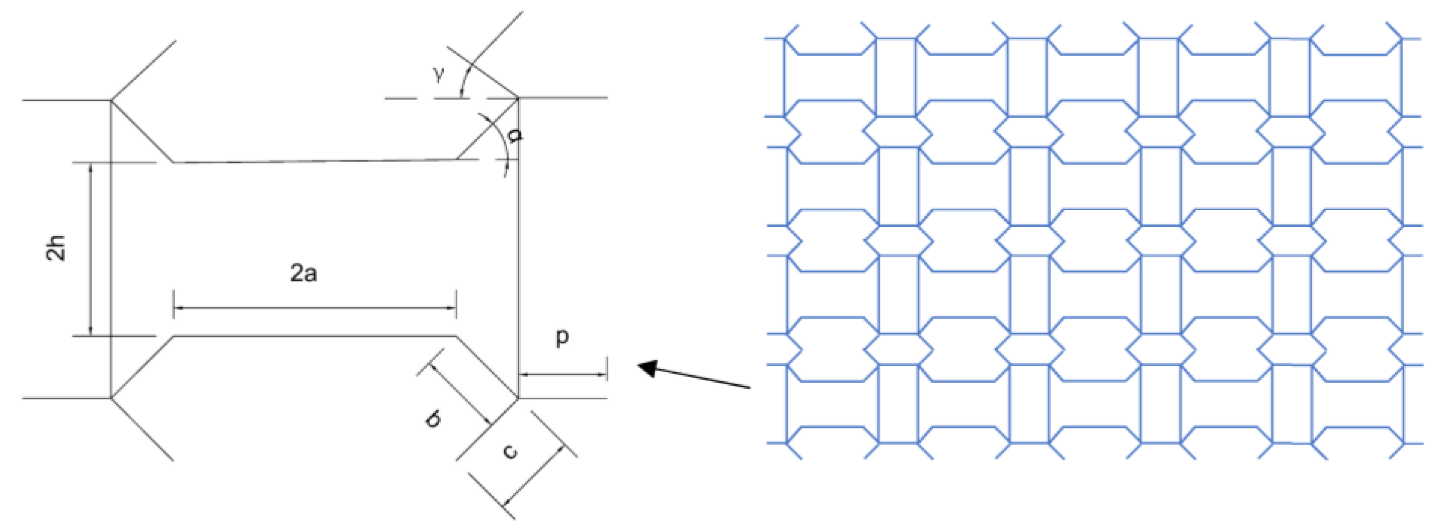
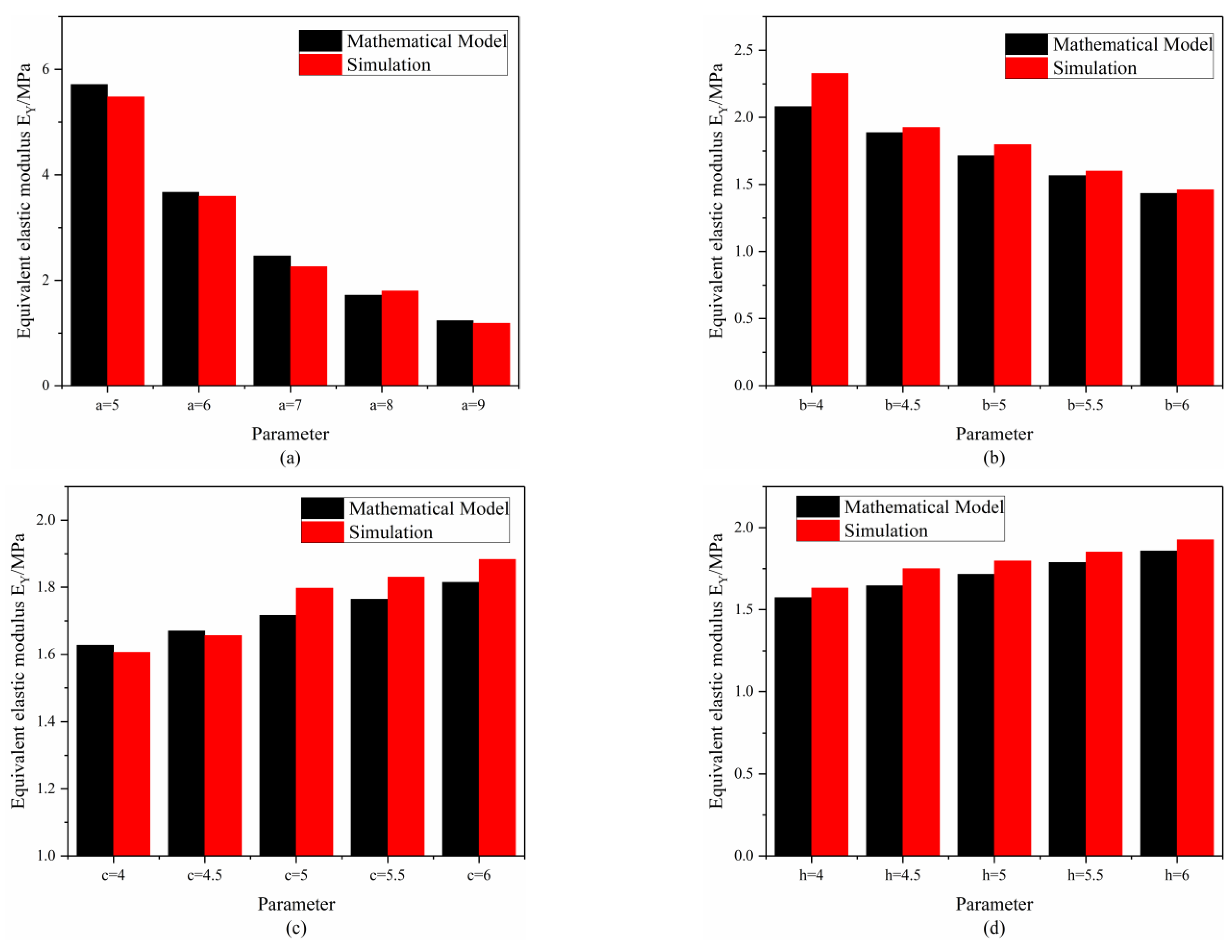
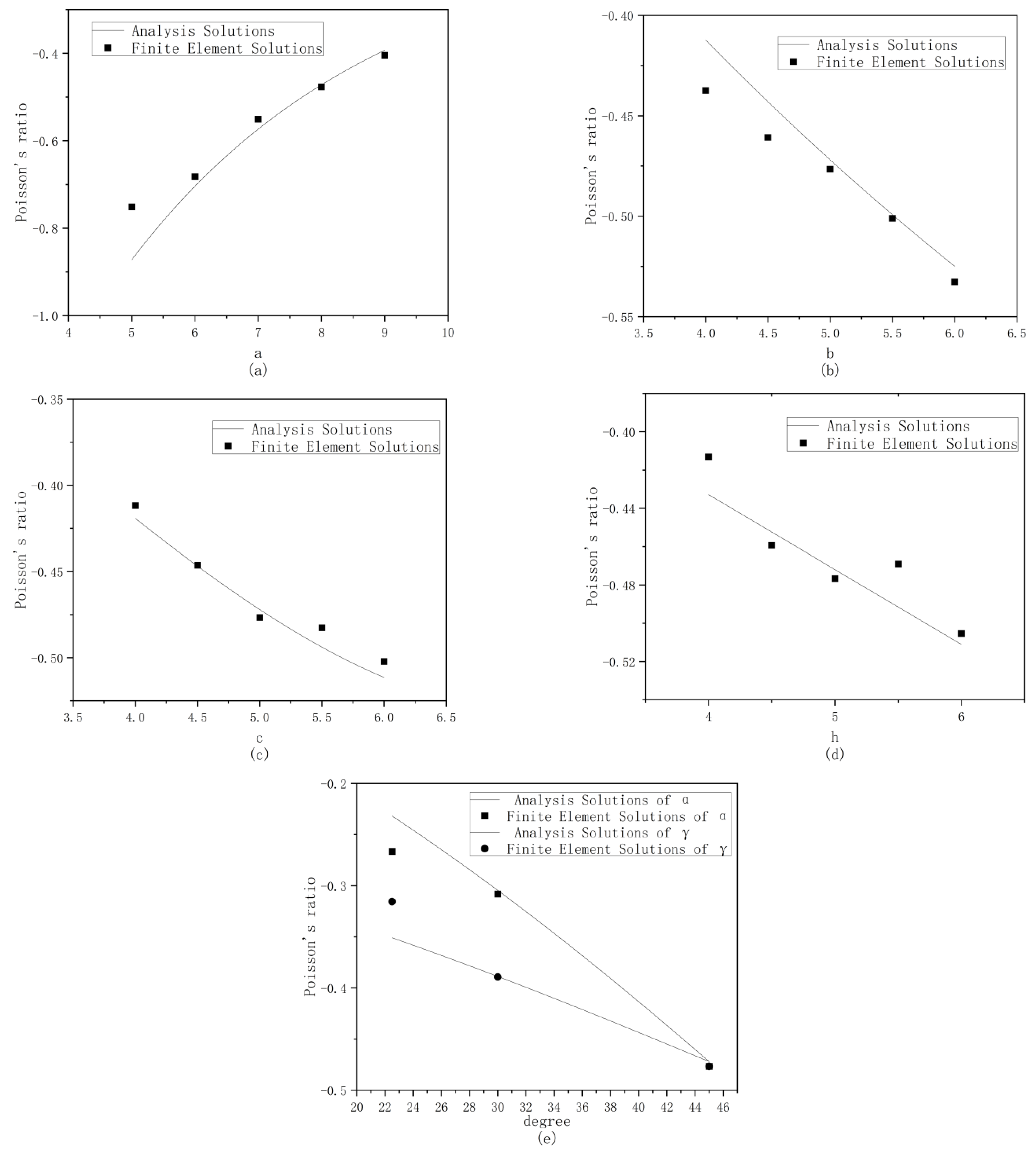
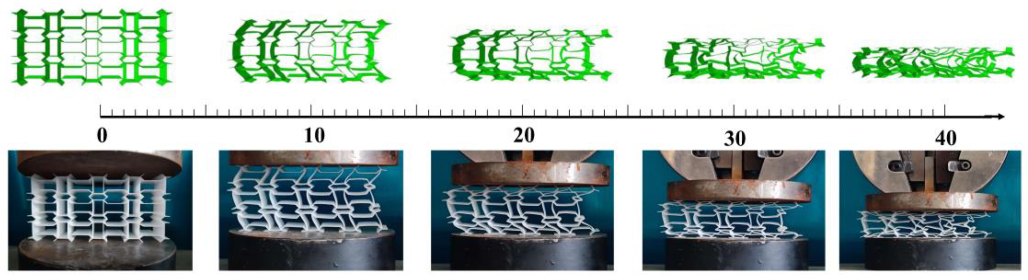
This article suggests modifying the optimization parameters in topology optimization to regulate the final structure, ensuring that it has a negative Poisson’s ratio. The mechanical properties of the structure were analyzed using theoretical, quasi-static compression, and finite element analyses. Following verification of the finite element model, numerical simulations examined the size of the concave beetle-inspired structure, including dimensions a, b, c, and h and angles α and γ.

Based on the results, increasing the size of a moderately reduced the specific energy absorption of the concave structure, exhibiting a linear relationship. The sizes of b and c nonlinearly impacted the specific energy absorption of the concave structure, with increasing b and c initially boosting and then lowering the specific energy absorption. Overall, the specific energy absorption of the structure fluctuated and decreased with increasing h, while α and γ values exerted a significant impact on the specific energy absorption of the structure. The results indicate that selecting structural dimensions considerably affects the specific energy absorption characteristics of the structure, and optimizing the structure’s design can enhance the energy absorption performance by up to 40% compared to the suboptimal case.

References

1. Smith, D.R.; Padilla, W.J.; Vier, D.; Nemat-Nasser, S.C.; Schultz, S. Composite medium with simultaneously negative permeability and permittivity. Phys. Rev. Lett. 2000, 84, 4184. [Google Scholar] [CrossRef] [PubMed] [Green Version]
2. Barchiesi, E.; Spagnuolo, M.; Placidi, L. Mechanical metamaterials: A state of the art. Math. Mech. Solids 2019, 24, 212–234. [Google Scholar] [CrossRef]
3. Carnap, R. Logik der Forfchung. Zur Erkenntnistheorie der modernen Naturwiffenfchaft. Erkenntnis 1935, 5, 290–294. [Google Scholar] [CrossRef]
4. Huang, Q.Q.; Wang, G.H.; Zhou, M.; Zheng, J.; Tang, S.L.; Ji, G.B. Metamaterial electromagnetic wave absorbers and devices: Design and 3D microarchitecture. J. Mater. Sci. Technol. 2022, 108, 90–101. [Google Scholar] [CrossRef]
5. Pendry, J.B. Negative refraction makes a perfect lens. Phys. Rev. Lett. 2000, 85, 3966–3969. [Google Scholar] [CrossRef] [PubMed]
6. Luo, X.H.; Hu, Y.Q.; Li, X.; Jiang, Y.T.; Wang, Y.S.; Dai, P.; Liu, Q.; Shu, Z.W.; Duan, H.G. Integrated Metasurfaces with Microprints and Helicity-Multiplexed Holograms for Real-Time Optical Encryption. Adv. Opt. Mater. 2020, 8, 1902020. [Google Scholar] [CrossRef]
7. Kudyshev, Z.A.; Kildishev, A.V.; Shalaev, V.M.; Boltasseva, A. Machine learning-assisted global optimization of photonic devices. Nanophotonics 2021, 10, 371–383. [Google Scholar] [CrossRef]
8. Gao, N.S.; Zhang, Z.C.; Deng, J.; Guo, X.Y.; Cheng, B.Z.; Hou, H. Acoustic Metamaterials for Noise Reduction: A Review. Adv. Mater. Technol. 2022, 7, 2100698. [Google Scholar] [CrossRef]
9. Zhou, Z.L.; Huang, S.B.; Li, D.T.; Zhu, J.; Li, Y. Broadband impedance modulation via non-local acoustic metamaterials. Natl. Sci. Rev. 2022, 9, nwab171. [Google Scholar] [CrossRef]
10. Zheng, Z.P.; Luo, Y.; Yang, H.; Yi, Z.; Zhang, J.G.; Song, Q.J.; Yang, W.X.; Liu, C.; Wu, X.W.; Wu, P.H. Thermal tuning of terahertz metamaterial absorber properties based on VO2. Phys. Chem. Chem. Phys. 2022, 24, 8846–8853. [Google Scholar] [CrossRef]
11. Yu, X.L.; Zhou, J.; Liang, H.Y.; Jiang, Z.Y.; Wu, L.L. Mechanical metamaterials associated with stiffness, rigidity and compressibility: A brief review. Prog. Mater. Sci. 2018, 94, 114–173. [Google Scholar] [CrossRef]
12. Wojciechowski, K.W. Auxetics and Other Systems with Unusual Characteristics. Phys. Status Solidi 2022, 259, 2200536. [Google Scholar] [CrossRef]
13. Wojciechowski, K.W.; Alderson, A.; Brańka, A.; Alderson, K.L. Preface: Phys. stat. sol. (b) 242/3. Phys. Status Solidi 2005, 242, 497. [Google Scholar] [CrossRef]
14. Kolpakov, A.G. Determination of the average characteristics of elastic frameworks. J. Appl. Math. Mech. 1985, 49, 739–745. [Google Scholar] [CrossRef]
15. Evans, K.E.; Nkansah, M.A.; Hutchinson, I.J.; Rogers, S.C. Molecular Network Design. Nature 1991, 353, 124. [Google Scholar] [CrossRef]
16. Bianchi, M.; Scarpa, F. Vibration transmissibility and damping behaviour for auxetic and conventional foams under linear and nonlinear regimes. Smart Mater. Struct. 2013, 22, 084010. [Google Scholar] [CrossRef]
17. Surjadi, J.U.; Gao, L.B.; Du, H.F.; Li, X.; Xiong, X.; Fang, N.X.; Lu, Y. Mechanical Metamaterials and Their Engineering Applications. Adv. Eng. Mater. 2019, 21, 1800864. [Google Scholar] [CrossRef] [Green Version]
18. Wojciechowski, K.W. Constant thermodynamic tension Monte Carlo studies of elastic properties of a two-dimensional system of hard cyclic hexamers. Mol. Phys. 1987, 61, 1247–1258. [Google Scholar] [CrossRef]
19. Wojciechowski, K.W. Two-dimensional isotropic system with a negative poisson ratio. Phys. Lett. A 1989, 137, 60–64. [Google Scholar] [CrossRef]
20. Hoover, W.G.; Hoover, C.G. Searching for auxetics with DYNA3D and ParaDyn. Phys. Status Solidi 2005, 242, 585–594. [Google Scholar] [CrossRef] [Green Version]
21. Wojciechowski, K.W. Non-chiral, molecular model of negative Poisson ratio in two dimensions. J. Phys. A Math. Gen. 2003, 36, 11765. [Google Scholar] [CrossRef]
22. Lakes, R. Deformation mechanisms in negative Poisson’s ratio materials: Structural aspects. J. Mater. Sci. 1991, 26, 2287–2292. [Google Scholar] [CrossRef]
23. Pozniak, A.A.; Wojciechowski, K.W. Poisson’s ratio of rectangular anti-chiral structures with size dispersion of circular nodes. Phys. Status Solidi 2014, 251, 367–374. [Google Scholar] [CrossRef]
24. Mizzi, L.; Attard, D.; Gatt, R.; Pozniak, A.A.; Wojciechowski, K.W.; Grima, J.N. Influence of translational disorder on the mechanical properties of hexachiral honeycomb systems. Compos. Part B Eng. 2015, 80, 84–91. [Google Scholar] [CrossRef]
25. Tretiakov, K.V.; Wojciechowski, K.W. Poisson’s ratio of the fcc hard sphere crystal at high densities. J. Chem. Phys. 2005, 123, 074509. [Google Scholar] [CrossRef]
26. Narojczyk, J.W.; Bilski, M.; Grima, J.N.; Kędziora, P.; Morozow, D.; Rucki, M.; Wojciechowski, K.W. Removing Auxetic Properties in f.c.c. Hard Sphere Crystals by Orthogonal Nanochannels with Hard Spheres of Another Diameter. Materials 2022, 15, 1134. [Google Scholar] [CrossRef]
27. Czarnecki, S. Isotropic material design. Comput. Methods Sci. Technol. 2015, 21, 49–64. [Google Scholar] [CrossRef] [Green Version]
28. Czarnecki, S.; Łukasiak, T. Recovery of the Auxetic Microstructures Appearing in the Least Compliant Continuum Two-Dimensional Bodies. Phys. Status Solidi 2020, 257, 1900676. [Google Scholar] [CrossRef]
29. Strek, T.; Jopek, H.; Idczak, E.; Wojciechowski, K.W. Computational Modelling of Structures with Non-Intuitive Behaviour. Materials 2017, 10, 1386. [Google Scholar] [CrossRef] [Green Version]
30. Bilski, M.; Pigłowski, P.M.; Wojciechowski, K.W. Extreme Poisson’s Ratios of Honeycomb, Re-Entrant, and Zig-Zag Crystals of Binary Hard Discs. Symmetry 2021, 13, 1127. [Google Scholar] [CrossRef]
31. Bilski, M.; Wojciechowski, K.W.; Stręk, T.; Kędziora, P.; Grima-Cornish, J.N.; Dudek, M.R. Extremely Non-Auxetic Behavior of a Typical Auxetic Microstructure Due to Its Material Properties. Materials 2021, 14, 7837. [Google Scholar] [CrossRef]
32. Bendsøe, M.P. Optimal shape design as a material distribution problem. Struct. Optim. 1989, 1, 193–202. [Google Scholar] [CrossRef]
33. Huang, X.; Xie, Y.-M. A further review of ESO type methods for topology optimization. Struct. Multidiscip. Optim. 2010, 41, 671–683. [Google Scholar] [CrossRef]
34. Da, D.; Xia, L.; Li, G.; Huang, X. Evolutionary topology optimization of continuum structures with smooth boundary representation. Struct. Multidiscip. Optim. 2018, 57, 2143–2159. [Google Scholar] [CrossRef]
35. Fu, Y.-F.; Rolfe, B.; Chiu, L.N.S.; Wang, Y.; Huang, X.; Ghabraie, K. SEMDOT: Smooth-edged material distribution for optimizing topology algorithm. Adv. Eng. Softw. 2020, 150, 102921. [Google Scholar] [CrossRef]
36. Huang, X. Smooth topological design of structures using the floating projection. Eng. Struct. 2020, 208, 110330. [Google Scholar] [CrossRef]
37. Lakes, R. Foam structures with a negative Poisson’s ratio. Science 1987, 235, 1038–1040. [Google Scholar] [CrossRef]
38. Xia, L.; Breitkopf, P. Design of materials using topology optimization and energy-based homogenization approach in Matlab. Struct. Multidiscip. Optim. 2015, 52, 1229–1241. [Google Scholar] [CrossRef]
39. Lee, D.; Shin, S. Evaluation of Optimized Topology Design of Cross-Formed Structures with a Negative Poisson’s Ratio. Iran. J. Sci. Technol. Trans. Civ. Eng. 2016, 40, 109–120. [Google Scholar] [CrossRef]
40. Chen, Y.; Ye, L.; Han, X. Experimental and numerical investigation of zero Poisson’s ratio structures achieved by topological design and 3D printing of SCF/PA. Compos. Struct. 2022, 293, 115717. [Google Scholar] [CrossRef]
41. Chatterjee, T.; Chakraborty, S.; Goswami, S.; Adhikari, S.; Friswell, M.I. Robust topological designs for extreme metamaterial micro-structures. Sci. Rep. 2021, 11, 15221. [Google Scholar] [CrossRef] [PubMed]
42. Sigmund, O.; Maute, K. Topology optimization approaches. Struct. Multidiscip. Optim. 2013, 48, 1031–1055. [Google Scholar] [CrossRef]
43. Wang, Y.F.; Sigmund, O. Multi-material topology optimization for maximizing structural stability under thermo-mechanical loading. Comput. Methods Appl. Mech. Eng. 2023, 407, 115938. [Google Scholar] [CrossRef]
44. Sigmund, O. Materials with Prescribed Constitutive Parameters—An Inverse Homogenization Problem. Int. J. Solids Struct. 1994, 31, 2313–2329. [Google Scholar] [CrossRef]
45. Li, Z.Y.; Wang, X.T.; Yang, J.S.; Li, S.; Schroder, K.U. Mechanical response and auxetic properties of composite double-arrow corrugated sandwich panels with defects. Mech. Adv. Mater. Struct. 2021, 29, 6517–6529. [Google Scholar] [CrossRef]
46. Steiner, W. The use of Castigliano’s theorem in Coulomb friction problems. Acta Mech. 2014, 225, 2471–2483. [Google Scholar] [CrossRef]
Figure 1. Initial structure for topology optimization.
Applsci 13 07728 g001
Figure 2. Variation in the objective function with the number of iterations for the six data sets. (a) Group A, (b) Group B, (c) Group C, (d) Group D, (e) Group E, (f) Group F.
Applsci 13 07728 g002
Figure 3. Unit cell configurations for group A under different β: (a) β = 0, (b) β = 0.002, (c) β = 0.004, and (d) β = 0.006.
Applsci 13 07728 g003
Figure 4. Unit cell configurations for group D under different β: (a) β = 0, (b) β = 0.004, (c) β = 0.008, (d) β = 0.010, and (e) β = 0.012.
Applsci 13 07728 g004
Figure 5. Unit cell configurations for group E under different β: (a) β = 0, (b) β = 0.005, (c) β = 0.010, (d) β = 0.020, and (e) β = 0.030.
Applsci 13 07728 g005
Figure 6. Variation in the objective function of the final topological columnar with the number of iterations.
Applsci 13 07728 g006
Figure 7. Variation in Poisson’s ratio of the final topological columnar with the number of iterations.
Applsci 13 07728 g007
Figure 8. Concave beetle-shaped structure.
Applsci 13 07728 g008
Figure 9. (a) The 1/4 cellular structure. (b) The internal forces of a 1/4 structure. (c) The 1/4 structure when only F/2 load is applied. (d) The 1/4 structure when acting only on unit bending moment. (e) Only horizontal unit forces acting on 1/4 of the structure.
Applsci 13 07728 g009
Figure 10. The original unit cell.
Applsci 13 07728 g010
Figure 11. (a) Effect of parameter a on the elastic modulus. (b) Effect of parameter b on the elastic modulus. (c) Effect of parameter c on the elastic modulus. (d) Effect of parameter h on the elastic modulus. (e) Effect of parameters α and γ on the elastic modulus.
Applsci 13 07728 g011aApplsci 13 07728 g011b
Figure 12. (a) Effect of parameter a on the Poisson’s ratio. (b) Effect of parameter b on the Poisson’s ratio. (c) Effect of parameter c on the Poisson’s ratio. (d) Effect of parameter h on the Poisson’s ratio. (e) Effect of parameters α and γ on the Poisson’s ratio.
Applsci 13 07728 g012
Figure 13. Impact on the negative Poisson’s ratio honeycomb structure.
Applsci 13 07728 g013
Figure 14. Test equipment.
Applsci 13 07728 g014
Figure 15. Structural compression processes: simulation and test.
Applsci 13 07728 g015
Figure 16. Comparison between simulation results and experimental results.
Applsci 13 07728 g016
Figure 17. (a) Effect of different a values on energy. (b) Effect of different a values on specific absorption energy.
Applsci 13 07728 g017
Figure 18. (a) Effect of different b values on energy. (b) Effect of different b values on specific absorption energy.
Applsci 13 07728 g018
Figure 19. (a) Effect of different c values on energy. (b) Effect of different c values on specific absorption energy.
Applsci 13 07728 g019
Figure 20. (a) Effect of different h values on energy. (b) Effect of different h values on specific absorption energy.
Applsci 13 07728 g020
Figure 21. (a) Effect of different α and γ values on energy. (b) Effect of different α and γ values on specific absorption energy.
Applsci 13 07728 g021