DroidDetectMW: A Hybrid Intelligent Model for Android Malware Detection

Abstract

Malicious apps specifically aimed at the Android platform have increased in tandem with the proliferation of mobile devices. Malware is now so carefully written that it is difficult to detect. Due to the exponential growth in malware, manual methods of malware are increasingly ineffective. Although prior writers have proposed numerous high-quality approaches, static and dynamic assessments inherently necessitate intricate procedures. The obfuscation methods used by modern malware are incredibly complex and clever. As a result, it cannot be detected using only static malware analysis. As a result, this work presents a hybrid analysis approach, partially tailored for multiple-feature data, for identifying Android malware and classifying malware families to improve Android malware detection and classification. This paper offers a hybrid method that combines static and dynamic malware analysis to give a full view of the threat. Three distinct phases make up the framework proposed in this research. Normalization and feature extraction procedures are used in the first phase of pre-processing. Both static and dynamic features undergo feature selection in the second phase. Two feature selection strategies are proposed to choose the best subset of features to use for both static and dynamic features. The third phase involves applying a newly proposed detection model to classify android apps; this model uses a neural network optimized with an improved version of HHO. Application of binary and multi-class classification is used, with binary classification for benign and malware apps and multi-class classification for detecting malware categories and families. By utilizing the features gleaned from static and dynamic malware analysis, several machine-learning methods are used for malware classification. According to the results of the experiments, the hybrid approach improves the accuracy of detection and classification of Android malware compared to the scenario when considering static and dynamic information separately.

1. Introduction

Smartphones have rapidly grown in popularity over the past decade, with billions of users, according to an analysis of Statista in 2021 [1]. The reason is that smartphones are so handy and convenient [2]. Sending emails, playing games, taking photographs and videos, searching the web, using GPS, and more are just some of the many uses for smartphones. Applications are being developed and improved daily, making it possible to achieve this, particularly on Android’s operating system, which first appeared as a hacked Linux kernel optimized for touchscreen mobile gadgets.

Moreover, last year Android OS apps extended to more than 3 million apps [3]. Banking, social media, healthcare, education, and entertainment are just some of the many possible uses for these Android apps [4]. As a result, most of these apps are employed to benefit their end consumers. Some of them, however, are used maliciously by hackers and exploiters. Malware refers to these harmful applications, defined as invasive software that steals data or causes damage to another user’s computer [5].

Cybercriminals create malware to function in many ways, including adware, worms, ransomware, and Trojan viruses [6]. Because malicious software is always evolving, it is increasingly challenging to foil security breaches [7]. For instance, in 2021, Cybersecurity Check Point warned Android users that millions of mobile smartphones were vulnerable to Agent Smith malware [8]. The spyware also uses WhatsApp as a cover to attack Android systems. In 2021, coccus reported that more than a billion Android smartphones would be vulnerable to hacking because they lacked the latest security upgrades [9]. Additionally, experts from Kaspersky Lab in 2020 found that numerous hackers had used the Google Play app store to spread complex malware [10] for years. Recently, many Facebook accounts were hacked using the android malware “FlyTrap” app [11].

The Android operating system has a built-in authorization module that checks whether or not a security policy has been breached before granting the permissions requested by an Android app. The four categories of Android permissions correspond to the four levels of security outlined in [12]. Also, the dataset includes four types of malware that may be labeled as such: ransomware [13] adware [14], SMS malware, and scareware [15]. The ever-expanding and changing nature of malware has prompted numerous proposals for detecting and avoiding it. The research community has revealed two methods for spotting malware. Static, dynamic, and hybrid malware analysis are three types of analyzing android malware. Static malware analysis is where applications are inspected without being run, while dynamic analysis evaluates the behavior of malware in a sandbox after it has been run [16]. Despite the role of current technologies in improving quality of life and expanding the cyber world, cyber-threats have reached a new level and are increasing at a scary rate [17]. More importantly, new attacks that can breach a smartphone’s defenses are constantly being developed and released.

Violating the security policy might take various forms, depending on the mobile device’s OS. This paper focuses on the Android operating system and new threats that threaten its security. The presence of malware in a mobile app has been investigated by several previous research [18,19,20,21,22], some of which made use of API calls and permissions. According to their findings, Dynamic analysis is also necessary since Static analysis is insufficient for detecting malware in obfuscated apps. It has been found in some research [23] that deep learning can be utilized to detect malware in mobile apps. This paper aims to provide a highly effective method for discovering and naming novel forms of malware, thus overcoming all these restrictions.

This is why we have put time and effort into Android malware detection and family classification. Here, “malware” and “benign” represent two classes in a binary classification problem, whereas “family classification” represents 13 classes in a multi-class classification problem. Android malware family refers to a collection of malicious apps that act similarly and are based on the same code. To identify and categorize malicious Android apps, we propose a hybrid classification. It depends on combining dynamic static malware analysis. At first, we run a static malware analysis to pull out static features like command strings, API calls, intents, and permissions. Then, we used CuckooDroid [24] to analyze dynamic malware to extract features. To do the automated analysis of suspicious Android files, CuckooDroid is an add-on to the cuckoo sandbox [25].

A standard method for malware detection using static and dynamic features, feature selection has received considerable attention [26]. Managing these massive datasets is no easy feat due to their complexity. It could hinder one’s learning ability or even lengthen the time. Feature reduction methods are essential to reduce the dimensionality of data because some attributes in datasets are unnecessary and redundant.

Accordingly, one of the most critical steps in developing a pattern classifier system is the feature selection phase, during which an appropriate feature subset is selected by analyzing possible feature subsets. For this reason, two feature selection strategies, static and dynamic, are proposed for the best possible malware classification in the used dataset. Using fuzzy logic [27,28] in conjunction with metaheuristic optimization, a two-stage feature selection strategy is proposed for selecting dynamic features. To detect and categorize An-droid malware applications, a hybrid model based on fuzzy optimization mixed with meta-heuristic optimization methods, hybrid of enhanced MFO [29] and MVO [30] is evaluated as wrappers. Three feature selection methods, fisher score, chi-square, and information gain, are applied to static features, eliminating more irrelevant features. Then, a subset of candidate features from both static and dynamic features was fed to several machine learning algorithms to produce the best detection results.

Several researchers have proposed artificial neural network (ANN) based models to replace more conventional approaches to malware detection and classification [31]. It has been shown that ANNs can model the relationships between inputs and outputs more accurately than other methods [32,33]. Additional restrictions on ANN use include difficulties in extrapolating beyond training data and overtraining the network due to extensive iterations during the training process. Therefore, the primary goals of this research are to (1) develop a better ANN model using the enhanced version of Harris Hawks optimizer (EHHO) and (2) check the accuracy of this model. The EHHO’s primary goal is to establish the optimal parameters for the ANN.

The following are the original contributions made by us in this paper:

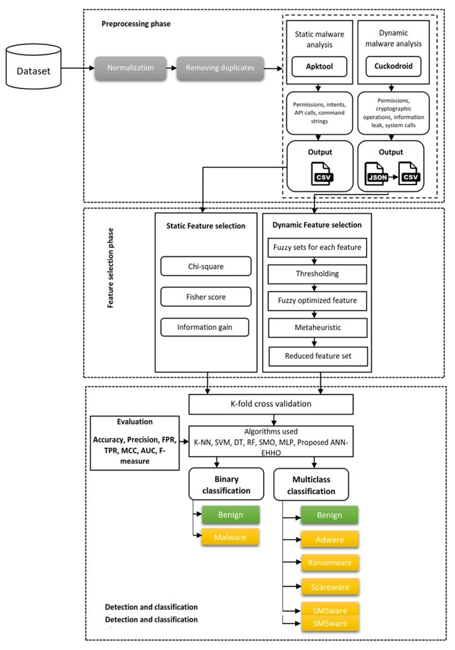
• DroidDetectMW is proposed as a functional and systematic model for detecting and identifying Android malware and its family and category based on a combination of Dynamic and Static attributes.
• Methods are proposed for selecting features, either statically or dynamically, to use.
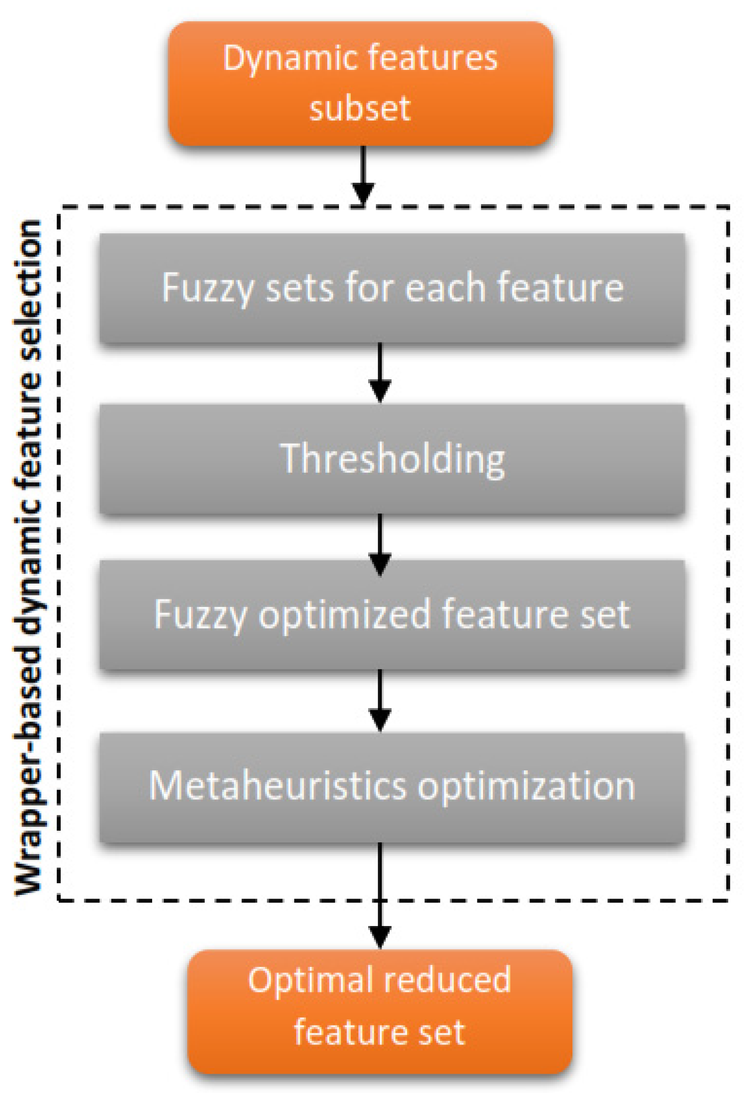
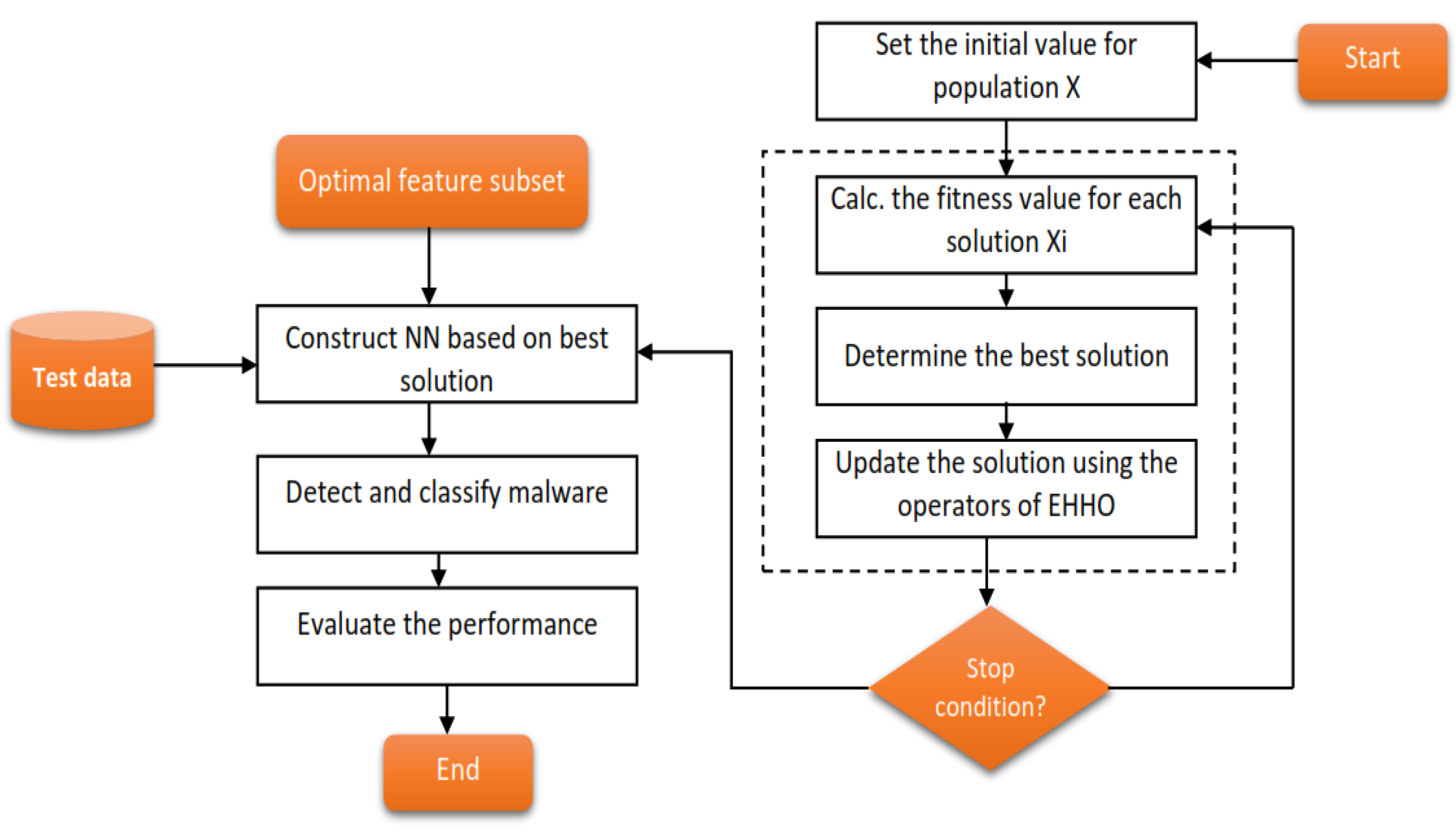
• A hybrid fuzzy-metaheuristics-optimization approach is proposed for selecting the optimal dynamic feature subset.
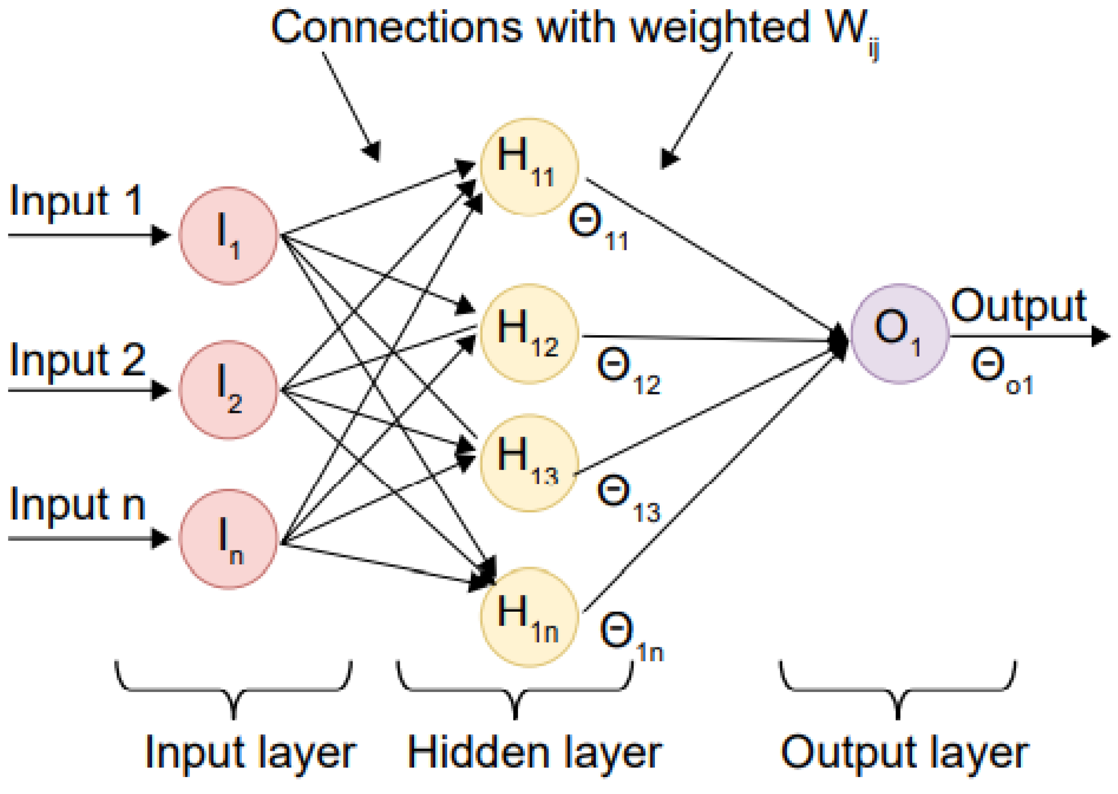
• An enhanced version of the HHO algorithm is proposed to optimize the parameters of ANN for malware detection.
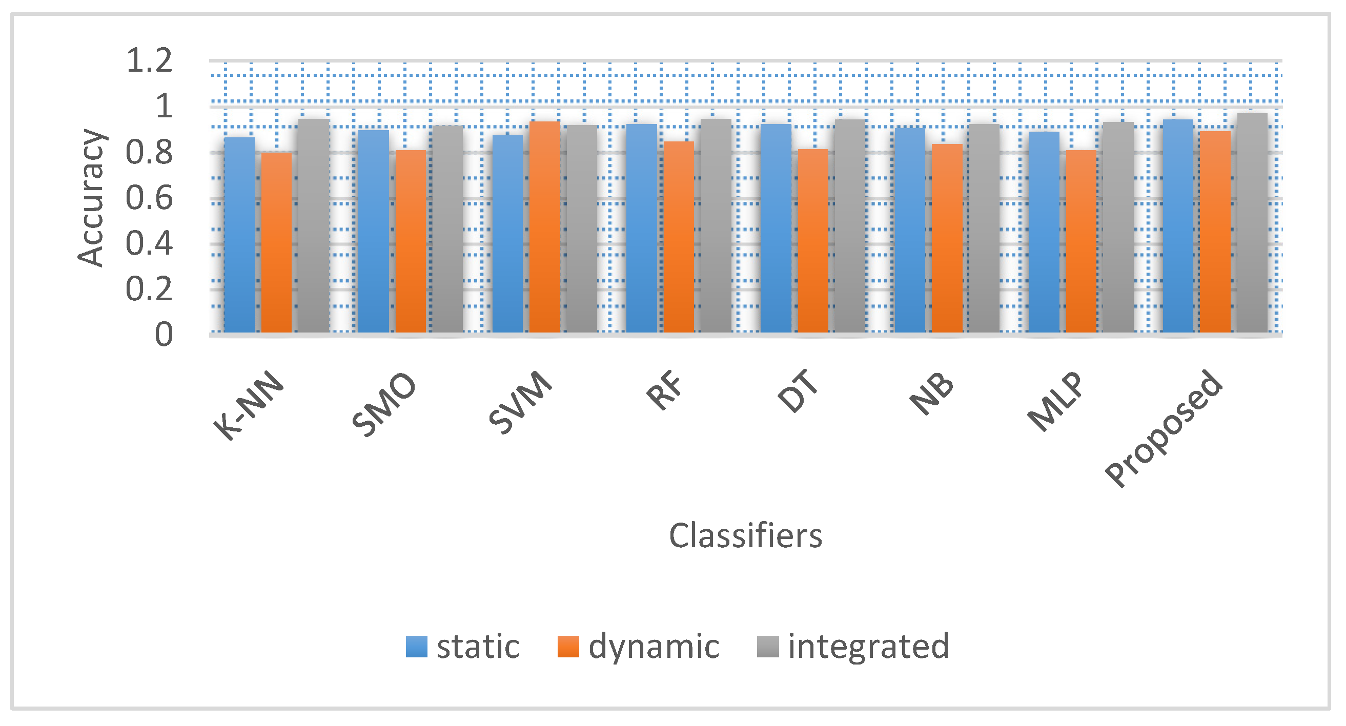
• A Comparison is applied between the results of the proposed Deep learning method with those of more traditional machine learning classifiers in determining how well DroidDetectMW works.
• Evaluate the performance of DroidDetectMW in comparison to seven traditional machine learning methods: the Decision Tree (DT), the support vector machine (SVM), the K-Nearest Neighbor, the Multilayer Perceptron (MLP), the Sequential Minimal Optimization (SMO), Random Forest (RF) and the Naive Bayesian (NB).
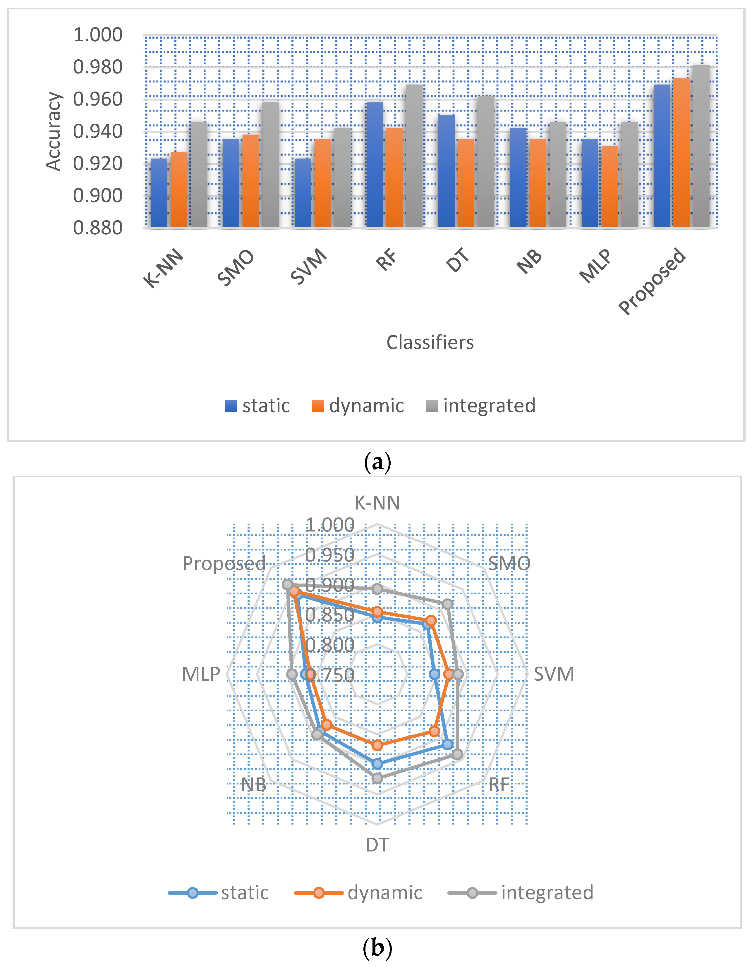
• Compared to traditional machine learning algorithms and state-of-the-art studies, DroidDetectMW significantly improves detection performance and achieves good accuracy on both Static and Dynamic attributes.

In the remaining sections of the study, the following structure is used: literature review and related work of previous studies are presented in Section 2. Understanding the fundamentals of Harris Hawks Optimization is covered in Section 3. In Section 4, we detail the methodology we’ll be using. Section 5 focuses on the experiments and findings, while Section 6 discusses the conclusion and directions for the future.

2. Related Work

Academics have published many ways to detect and categorize Android malware with ML algorithms. This paper will review the tasks involved in malware detection and classification using ML and deep learning techniques, including static and dynamic malware analysis.

In [34], Significant Permission Identification SigPID is a malware detection approach proposed by Li et al. They construct a three-tiered pruning system based on extracted permission data to identify malicious apps from legitimate ones. The Android apps were categorized by the authors using ML methods. According to the experiments, SigPID has a 93.62% higher efficiency than the best existing approaches.

In [35], the authors delved into the threats posed by Android apps’ need for permissions. T-tests, mutual information, and correlation coefficients were used to sort the risks associated with each permit. The subgroups of potentially malicious permissions are identified using sequential forward selection and principal component analysis (PCA). A decision Tree, Support Vector Machine, and Random Forest were used to evaluate how well risky permission could identify malicious apps. From what we can see, this detector has a 94.62% detection accuracy and a 0.6 False Positive Rate (FPR).

Regarding enhancing accuracy, the innovative fusion technology (DroidFusion) introduced by Yerima and Sezer [36] is hard to beat. DroidFusion trains classifiers to construct a model, which is then used with a feature importance ranking method based on the prediction precisions to obtain a classifier. The experiments highlight DroidFusion’s superiority over the stacking ensemble technique.

The methodology suggested by Das et al. [37], frequency centric for feature creation utilizing system calls, can accurately identify malware through only those system calls. The authors create an MLP on FPGA-based ML methodology for classifier training. The suggested method was determined to achieve high precision, rapid detection, and low power usage.

Automatically classifying the app as malicious or benign, the authors in [23] built an engine called DroidDetector. Using dynamic and static analysis, the authors extracted the features. Finally, the experimental results show that DroidDetector has the highest accuracy of 96.76% compared to traditional ML methods.

The Android Application Sandbox (AASandbox) was introduced by the authors of [38], which can perform both static and dynamic analysis to aid in detecting malicious apps. They used cloud deployment of the detection algorithm and sandbox to provide widespread and fast detection. The outcomes show that AASandbox performs better than Android antiviral apps.

In [39], the authors create a hybrid sequential network architecture using stacked denoising auto-encoders (SDAEs) and stacked hybrid learning merged sparse auto-encoders (MSAEs). Feature extraction from this hybrid model is fed into classification techniques like the SVM and K-NN. Using two datasets, the proposed model is compared to various previous detection methods using evaluation metrics such as precision, accuracy, f1-score, specificity, and sensitivity.

Malware classification is proposed in [40], which presents a DeepMal model for malware detection based on a combination of LSTM and CNN deep learning models. The data for this model was derived from a similar source—a sequence of API calls. This hybrid CNN-LSTM design features a variety of layers, including a nonlinearity layer, a convolution layer, and a whole layer. There is a significant probability of malware assaults due to the massive volumes of data uploaded to the cloud.

Metrics for assessing the efficacy of a model for detecting malware in the cloud are presented in [41]. A two-dimensional convolutional neural network (CNN) model supplied with memory, CPU, and network information yielded 90% accuracy. Furthermore, the SMOTE method and standardization with hyper-parameter adjustment can be used to achieve excellent detection accuracy. For research purposes, the Cuckoo sandbox has collected logs of API calls made by dynamic malware.

Using the deep learning model called Convolutional Neural Network (CNN), the authors of this research [42] present a malware detection model and compare it to existing machine learning classification models SVM, MLP, and RF. Netmate transforms publicly available data into flow information regarding the Stratosphere IPS project. The feature extractor Netmate was employed. Regarding accuracy, precision, and recall, CNN and random forest algorithms perform best.

3. Preliminary

3.1. Harris Hawks Optimization (HHO)

HHO was developed by [43], and it is a population-based optimization method with inspiration drawn from the natural world. Harris’ hawks’ cooperative chasing of prey, known as the surprise pounce, is an inspiration for HHO. Hawks use this strategy by swooping in from all sides to catch their prey off guard. The HHO consists of two primary phases: exploitation and exploration and a transition between exploitative actions. The hawks in the desert are the potential solutions, and the prey they’re waiting for is the best at each stage. Harris’ hawks begin their haunting by randomly picking areas and waiting to see whether they can detect any prey during the exploring phase. The first method relies on the locations of other hawks also involved in haunting the prey, whereas the second relies on the absence or presence of tall trees within the haunt range.

In both cases, the decision is based on the first strategy being chosen if q ≥ 0.5 and the second strategy being chosen if q < 0.5. The vector of hawk positions in the next cycle is defined as X(t + 1). The current iteration’s prey position is denoted by X_rabbit (t), a hawk’s position is chosen at random using X_rand (t), and the hawks’ positions are represented by X(t). Lower and upper bounds LB and UB are iteratively updated for the random values r₄, r₂, r₁, r₃, and q in the interval (0,1) as shown in Equation (1).

$$x(t+1)=\left\{\begin{array}{cc}{X}_{\mathrm{rand}}\left(t\right)-r_1\mid X_{\mathrm{rand}}\left(t\right)-2r_{2}X\left(t\right)|& q\ge 0.5\\ \left(X_{\mathrm{rabbit}}\left(t\right)-X_m\left(t\right)\right)-r_3\left(LB+r_4(UB-LB)\right)& q<0.5\end{array}\right.$$

(1)

Equation (2) can be used to determine the mean position of the current population of hawks, denoted by the symbol X_m(t). Where X_i(t) defines the position of the hawk i in recent iteration, and N is the whole number of hawks.

$$X_m(t)=\frac{1}{N}\sum _{i=1}^N X_i\left(t\right)$$

(2)

During the exploitation stage, Harris’ hawks initiate attacks on victims using the surprise pounce. In response to repeated attempts at evasion by their victim, hawks modify their pursuit strategies. As a result, hawks employ four distinct chasing strategies: the Soft Besiege, the Hard Besiege, the Hard Besiege with progressive rapid dives, and the Soft Besiege with progressive quick dives.

As the victim expends energy to flee the haunt, its remaining reserve determines which of the four strategies it will employ. This means that the individual can switch between several forms of exploitation. Equation (3) is a valid modeling of the energy of the prey, where T is the highest number of iterations with E₀ is the initial energy of the prey.

$$E=2E_0\left(1-\frac{t}{T}\right)$$

(3)

The soft besiege takes place when |E| ≥ 0.5 and if the prey has a probability of r ≥ 0.5 of being able to leak from the hawks. If r < 0.5, then the soft besiege strategy with progressive rapid dives is employed. Both approaches are shown in Equations (4) and (5), respectively. The instruction to assess the hawks’ next move during a soft besiege is denoted by Y, where ΔX(t) represents the difference between the rabbit’s position vector and the location stored in the current iteration t, $J=2(1-r_5)$ that denotes the varying magnitude of the rabbit’s leaps during the process of its escape. Only if the Y rule isn’t successful may the misleading zigzag motion shown in the Levy Flight LF move be used. Readers can find Z, Y, and LF in the original literature.

$$X(t+1)=\mathsf{\Delta }X\left(t\right)-E\left|J{X}_{\mathrm{rabbit}}\left(t\right)-X\left(t\right)\right|$$

(4)

$$X(t+1)=\left\{\begin{array}{ll}Y& \mathrm{if}F\left(Y\right)<F\left(X\right(t\left)\right)\\ Z& \mathrm{if}F\left(Z\right)<F\left(X\right(t\left)\right)\end{array}\right.$$

(5)

If |E| < 0.5, then the Hard besiege strategy is used, provided that r ≥ 0.5. In that case, a hard be-siege with progressive quick dives will be applied. For hard besiege with advanced rapid dives, the same Equation (5) is employed, except that Y considers the average locations of the hawks instead, as shown in Equation (6).

$$X(t+1)=X_{\mathrm{rabbit}}\left(t\right)-E\left|\mathsf{\Delta }X\right(t\left)\right|$$

(6)

3.2. Dataset and Malware Categories

We determined that the Canadian Institute for Cybersecurity (CIC) [44] offers a competent real-world dataset named CICAndMal2017 after examining the most comprehensive and coherent set of related papers. First, the CIC amassed around 4000 malware apps from various sources as Contagiodumpst [45] and VirusTotal [46]. In addition, nearly 6000 benign apps from 2015 to 2017 that were uploaded to the Google Play market were collected. CIC has only been able to install 5000 (benign 5065 and malware 429) on actual An-droid smartphones to undertake real-world scenario testing. Several articles make use of the Drebin dataset. A total of 5560 apps from 179 distinct malware families are included in this data collection. The MobileSandbox project generously provided us with samples gathered between August 2010 and October 2012. A total of 4890 recent Android apps were downloaded from virusshare and apkmirror and selected from DREBIN, CICInvesAndMal2017, datasets of them there are 1910 samples of malware and 2980 samples of benign. The used dataset consisted of static and dynamic features to evaluate the proposed model. The realm of malicious software encompasses a plethora of classifications, ranging from worms and viruses to adware, spyware, Trojans, SMSware, Ransomware, and various other insidious variants.

In this data set, labels can be found at various depths. Beginning with a binary classification system, files are either malware or benign. The CICAndMal2017 dataset comprises both benign and malware applications. It includes four distinct categories of malware, namely Adware, SMS Malware, Scareware, and Ransomware. There are four categories of malware in the second level:

• Adware: To generate as much revenue as possible from unsolicited banner ads, the ad-ware will display these ads automatically [47].
• Ransomware: One goal of malicious software is to prevent apps from accessing system resources. To extort money from users, it can encrypt their files and demand payment before allowing them to access their files or recover their devices [48].
• Scareware: This malware software uses scare tactics to convince users to buy bogus security updates [49].
• SMS malware: A malicious malware that makes sms calls and sends text messages with-out the user’s permission. The malware operator can use the compromised handsets as a high-end SMS distribution channel [50].

4. Proposed Framework

Here, we’ll review the recommended process for locating and categorizing Android apps by family. Data preprocessing, feature selection, detection, and family categorization are its three main phases. The feature values are normalized in the first phase, and duplicate apps are removed from the dataset. Then, feature extraction of both static and dynamic malware features is applied. In this phase’s end stage, the extracted features are vectorized and put in binary vectors for further processing. He pulled static characteristics, including Command strings, API calls, intents, and permissions. Extracted elements from dynamic malware analysis include cryptographic activities, dynamic approvals, system calls, and information leakage. In the second phase, feature selection is employed for static and dynamic features extracted from the feature extraction stage. Three filter approaches are applied for static attributes, and the optimum feature subgroup is selected. For dynamic features, a two-stage fuzzy-metaheuristic method is applied to attain the best set of dynamic features. In the third phase, a proposed deep learning approach based on enhanced HHO is used to categorize the categories of malware and families. Then, the Android apps are identified and classified using the proposed detection approach against several distinct classifiers based on machine learning and deep learning, such as SMO, RF, DT, K-NN, NB, SVM, SMO, and MLP. The process flow of the proposed approach is pro-posed in Figure 1.

4.1. Data Pre-Processing

The best results from a machine learning or deep learning model can only be achieved after extensive preprocessing. Duplicate instance cleanup, NaN removal, and normalization/scaling are all examples of everyday preprocessing operations. We use MinMax scaling to normalize the features because the given dataset has minimal variance and ambiguity. The term normalizing describes the operation of rescaling values with a fundamental number component to a speci-fied interval (e.g., 0 and 1). If your model depends on the absolute values of inputs, you must ensure that they are appropriately scaled. Data is normalized by applying the formula presented in for MixMax scaling using Equation (7):

$$X_{\mathit{norm}}=\frac{X_i-X_{min}}{X_{max}-X_{min}}$$

(7)

where X_i is the feature’s initial value, the denominator represents the difference between the feature’s new normalized maximum and minimum values.

To filter out duplicates, the gathered Android apps are hashed using the MD5 method. There are now only 3514 unique Android apps after the copies have been removed, which consists of 1479 samples of malware and 2035 samples of benign.

Features can be extracted from malware using both dynamic and static analysis. According to the analysis of static features, we have collected intents, API calls, command strings, and permissions using a custom-written python script that uses the Apktool tool. According to the analysis of dynamic features, we have used CuckooDroid to extract dynamic permissions, cryptographic operations, system calls, and information leakage.

4.2. Feature Selection

It’s a tool for reducing the number of dimensions in a problem, which aids in selecting the most critical aspects—lowering the quality and accuracy of a classification model, and irrelevant and redundant features might have. More processing time and storage were needed for higher-dimensional datasets [51]. The time and space complexity can be reduced and the accuracy improved by selecting the necessary features. We have used feature selection methods that consider both static and dynamic features in this paper. The features that are generated as a byproduct are the most helpful set of features for the subsequent classification and detection processes. The results demonstrated that combining static and dynamic attributes is superior to using either alone. To eliminate and decrease the unnecessary static features, three filter techniques were employed to generate three candidate subsets; the best of these was then used for static feature selection. To select the optimal feature subset of dynamic features, a two-stage hybrid metaheuristic optimization algorithm using a fuzzy approach is proposed. More specific instructions for doing so are provided below.

To rationally evaluate the static features and improve the algorithm’s performance, feature selection is required. We use a filter-based methodology to ensure that feature selection does not rely on the underlying detection technique. See Algorithm 1 for further explanation. Three potential feature subsets were obtained using the chi-square test, the Fisher score, and the mutual information gain. The detection models are further compared in terms of their performance on the three feature subsets to determine which one is the most effective. The optimal detection model is chosen by averaging the results of various algorithmic models applied to the feature subset. The optimal feature subset is then selected by examining the effects of the chosen optimal model applied to the different feature subsets. Using experimental results, the chi-square test is the superior technique for determining features using the random forest anomalies detection model. The above methods were implemented using scikit-learn [52] a Python machine-learning package.

This study proposes combining fuzzy and meta-heuristic optimization to eliminate redundant information and improve performance. Both fuzzy benchmarking and meta-heuristic optimization techniques, such as Multi-Verse Optimization (MVO) and Enhanced Moth Flame Optimized (EMFO), executed within Machine Learning (ML) wrappers, are utilized to discover the best features.

Algorithm 1: static-feature-select

Input: Training dataset D with static features S Output: optimal subset of features Snew  1. def static-feature-select(D,S):  2. Calculate feature importance using chi-square, fisher and information gain from S  3. S1 = remove features with score 0 and NaN from chi-s  4. S2 = remove features with score 0 and NaN from fisher  5. S3 = remove features with score 0 and NaN using MIG  6. A = avg-perf-model(S1,S2,S3)  7. M = best-subset(S1,S2,S3)  8. S = best-subset(S1,S2,S3)  9. return Snew  10. End def

In Figure 2, we see a schematic of the proposed dynamic feature selection framework. This phase generates fuzzy sets for each feature retrieved in the previous phase [23]. To get the fuzzy optimal feature set, each feature’s standard deviation (SD) is computed and compared to a threshold value. Fuzzification filters feature before sending them on to metaheuristic swarm optimization methods [53]. Following classification, the reduced feature set is sent into machine learning algorithms for testing their ability to categorize the dynamic features into benign and malicious categories. While there are various feature optimization techniques to choose from, we have focused on MVO and MFO due to their lack of attention in the mal-ware detection literature. Following is a breakdown of the proposed hybrid method:

A fuzzy set [54] is a collection of things with varying degrees of membership. Each item in this set is given a membership degree between 0 and 1 according to the membership function defined by this set [55].

Let’s write down the labeled data set as $H$, where $h$ is a member of $H$. With its definition in Equation, the fuzzy set $A$ defined on $H$ is a set of sorted pairs as in Equation (8):

$$A=\left\{x,{\mu }_A(x;a,b,c,d)\right\},x\in X$$

(8)

As demonstrated in Equation (9) and (10), a trapezoidal membership function, ${\mu }_{}(x;a,b,c,d)$ is used to project each element $h$ into fuzzy space:

$${\mu }_{\mathrm{trapezoidal} }(h;a,b,c,d)=\left\{\begin{array}{c}0,h\le a\\ \frac{h-a}{b-a},a\le h\le b\\ 1,b\le h\le c\\ \frac{d-h}{d-c},c\le h\le d\\ 0,d\le h\end{array}\right.$$

(9)

$${\mu }_{\mathrm{trapezoidal} }(h;a,b,c,d)=m\left(m\left(\frac{h-a}{b-a},1,\frac{d-h}{d-c}\right),0\right)$$

(10)

With quantile values of 0.100, 0.25, 0.50, and 0.75 for this characteristic, a, b, c, and d have been chosen to represent them. By taking the Mean, Median, Mode, Standard Deviation, and Variation into account, Sandya et al. [56] conducted research in the field of fuzzification. Based on their research, we have investigated using SD as a parameter in our lab work. The resultant fuzzy set is next parsed into its constituent features, and each feature’s standard deviation is determined and represented using Equation (11):

$$Z=\left[z_1,z_2,z_3,\dots ,z_n\right]$$

(11)

where $n$ is the whole number of features, each feature of $Z$ that satisfies the criterion in Equation (12) below is considered an optimized feature.

$$Z_i>T$$

(12)

A threshold value $T\in \left[\mathrm{0,1}\right]$ is shown above, with $i=[\mathrm{1,2},3,...,n]$. In this study, we calculated the thresholds using the SD that is constantly on the move throughout a certain time period. By using trial and error, we investigated possible threshold values between 0 and 1. The optimal values for threshed was determined through trials and errors during experimentations as 0.47, 0.48, 0.49. There are several methods for optimizing features, and picking one that works well requires consideration of many different criteria, such as the available optimization time, the number of parameters, and the amount of space required.

4.3. Detection and Family Classification

This section introduces the proposed detection approach and the comparative results with other machine learning models.

As mentioned in Section 2, the HHO algorithm is based on observations of how different Harris hawks approach prey. A solution’s efficacy determines how quickly HHO moves between exploitation and exploration. When it comes time to exploit the catch, Hawk swoops in for the kill.

Despite the remarkable performance of basic HHO, through simulations, we learn that improving both the exploration and exploitation processes improves the original HHO. Incorporating a QRL technique has been shown to improve both intensification and diversification.

A mechanism recognized as quasi-reflection-based learning (QRL) has developed in recent research as a potentially useful approach to increasing exploration, balancing exploitation and exploration, and accelerating convergence [57]. It has been recognized as an effective approach in the field, showcasing its potential for advancing learning algorithms.

To generate the quasi-reflected component, denoted as $x_j^{qr},$ of solution x, the following process is employed:

$$X_j^{qr}=\mathrm{r}\mathrm{n}\mathrm{d}\left(\frac{L{B}_j+U{B}_j}{2},X_j\right)$$

(13)

where $\mathrm{rnd}\left(\frac{L{B}_j+U{B}_j}{2},x_j\right)$ generates random numbers from a uniform distribution in the range $\left[\frac{L{B}_j+U{B}_j}{2},X_j\right]$, and $\frac{L{B}_j+U{B}_j}{2}$ calculates the average of the upper and lower bound for every parameter $j$.

Each iteration ends when, a quasi-reflected solution $x_i^{qr}$ is generated for each individual $i$ in the entire population $P$, which consists of $N$ individuals. This leads to the formation of a quasi-reflected population $P^{qr}$. Eventually, the populations $P$ and $P^{qr}$ are combined, and the solutions in this merged population are sorted in descending order based on their fitness. The top N individuals are then selected for propagation to the next iteration.

To improve upon both the worst X_worst and best solution X_best, the proposed method employs the QRL at each iteration. Where, X_best and X_worst are replaced by $X_{\mathrm{best} }^{qr}$ and $X_{\mathrm{worst} }^{qr}$ respectively, if and only if $X_{\mathrm{best} }^{qr}$’s fitness is greater than the previous best solution.

The proposed method for the malware families and categories detection phase using EHHO-ANN is depicted in Figure 3.

In this classification, models for identifying and categorizing Android malware are construct-ed using a wide range of ML techniques (including RF, SVM, DT, SMO, K-NN, MLP and NB). To gauge the efficacy of our proposed method, we employ these models for analysis. To train these models, the entire dataset is split into five sections called “folds.” Every part of the model is run, four pieces are utilized for training, and the remaining two are used for testing. Brief descriptions of ML algorithms and the criteria by which they are judged are provided here.

In this work, we used the following machine-learning algorithms:

• K-Nearest Neighbors (K-NN) is a simple supervised learning technique. This concept shares terminology with the lazy learner [58]. This technique does not care about the underlying data structure when a new instance appears. Instead, it uses distance measurements (e.g., Euclidean distance, Manhattan distance) to determine which training samples are most similar to the incoming instance. Majority voting notions ultimately determine this new instance’s class.
• Sequential Minimal Optimization (SMO) takes a set of points as its input. The method generates a hyperplane that separates points within the same class by analyzing the gaps between them. Kernel functions fill in the blanks in SMO by revealing data about the distance between two spots.
• SVM is a technique [59] that uses a hyperplane to partition the information. In a nutshell, it’s a dividing line from which to choose. Distances between the nearest data points are called support vectors, and the hyperplane is calculated randomly after the hyperplane is drawn. It searches for the optimal hyperplane that maximizes the profit.
• Random Forest (RF): A considerable number of independent decision trees are used in RF to form a unified whole [60]. Each decision tree generates an output classification for the input data, then compiled by RF and represented graphically based on a majority vote.
• A Decision Tree (DT) is organized in the form of a tree, where each node (whether internal, leaf, terminal) represents a test on an attribute, and each branch (whether internal, leaf, or terminal) carries a class name and the results of the test. The C4.5 algorithm has been utilized in this work to categorize Android malware [61].
• Bayes’ theorem provides the theoretical foundation for the NB idea. The program predicts the probabilities of class membership or the likelihood that a set of tuples belongs to a specific class. Multi-class and binary classification problems [57] both benefit from their application.
• Multilayer Perceptron (MLP): There are the hidden and output layers and the input layer. It can produce results in several different measurement systems. The hidden layer’s output units are fed into the subsequent layer as input applied deep learning approaches like ANNs classifiers to various classification challenges. The authors use MLP to identify and categorize Android malware when classifying and predicting gait data. The MLP is executed using a hidden layer of h = 3 and sigmoid activation function for the binary classification and h = 5 and softmax activation function for the multi-class classification. Learning is assumed to occur at a rate of 0.35. For a high-level overview of how backpropagation works in a neural network, see Figure 4.

5. Experiments

Specifically, we conduct three primary experiments to measure the efficacy of the proposed DroidDetectMW: The first experiment, detection, and identification, is to determine whether or not a specific app is a malware; the second experiment seeks to identify the family of malware, and the last one is the impact of feature selection proposed approach for both static and dynamic features. In the previous experiment, a comparison between with and without feature selection approaches is applied over different models, including the proposed detection approach. To begin, we divide the dataset into two classes: malware and benign apps. Ransomware, SMS malware, scareware, and adware samples comprise the four categories of malware used in the second stage of classification of the dataset. The data set is further annotated with labels for 13 families of malware as shown in

Table 1. Malware family types used.

Malware Family Types	Malware Category	# of Samples
Ewind	Adware	154
Kemoge	Adware	153
Dowgin	Adware	176
Zsone	SMSmalware	105
Jisut	Ransomware	117
Svpeng	Ransomware	116
AndroidDefender	scareware	133
FakeAV	scareware	103
Penetho	scareware	142
Biige	SMSmalware	174
SMSsniffer	SMSmalware	181
Youmi	Adware	164
Ginmaster	Adware	192

.

Table 2. Distribution of used samples of dataset.

Dataset	Number of Samples	#of Malware Samples	# of Benign Samples
Drebin	1400	450	950
CICAndMal2017	1240	450	790
APKMirror	1200	410	790
VirusShare	1050	600	450
Total	4890	1910	2980

offers a comprehensive breakdown of the collected samples utilized to construct the data set.

5.1. Evaluation Measures and Experimental Setup

Several measures are used to evaluate the classifiers’ efficacy, such as Matthews correlation coefficient (MCC), precision, F-measure, true positive rate (TPR), Area under curve (AUC), and false positive rate (FPR). The evaluation measures are based on false positive (FP), true negative (TN), true positive (TP), and false negative (FN). We used 20% of the data during the experiment for testing, while 80% was for training. The following Equations provide further information. The experimental computing setup is listed in

Table 3. The experimental environment settings.

Setting	Parameter
PU	Intel(R) Core(TM)i7-2.40 GHz
Operating System	Windows 10 Home Single
GPU	NVIDIA 1060
RAM	32 GB
Python Version	3.8

. For dynamic features, it also shows that certain families of malware are tailored to ARM devices and hence cannot run on x86 emulation. Consequently, in such scenarios, the use of emulator sandboxes for studying and detecting these families becomes impractical, restricting the effectiveness of emulators as platforms for forensics and detection.

• TPR—Recall: It is calculated by dividing the number of confirmed positive results by the total number of positive results. As illustrated in Equation, it can be estimated by Equation (14):

$$\mathit{T}\mathit{P}\mathit{R}=\frac{\mathit{T}\mathit{P}}{\mathit{T}\mathit{P}+\mathit{F}\mathit{N}}$$

(14)

• FPR: This metric represents the proportion of false positive cases relative to the total number of true negative cases. The calculation is described by the following Equation (15):

$$\mathit{F}\mathit{P}\mathit{R}=\frac{\mathit{F}\mathit{P}}{\mathit{T}\mathit{N}+\mathit{F}\mathit{P}}$$

(15)

• Precision is calculated by dividing the number of correct predictions by the total number of correct predictions. It can be calculated by Equation (16):

$$\mathit{P}\mathit{r}\mathit{e}\mathit{c}\mathit{i}\mathit{s}\mathit{i}\mathit{o}\mathit{n}=\frac{\mathit{T}\mathit{P}}{\mathit{T}\mathit{P}+\mathit{F}\mathit{P}}$$

(16)

• F-measure: It indicates the harmonic mean of precision and recall. Equation (17) is used to deter-mine this is:

$$\mathit{F}-\mathrm{measure}=\frac{\mathbf{2}\times (\mathrm{Precision}\times \mathrm{Recall})}{(\mathrm{Precision}+\mathrm{Recall})}$$

(17)

• Accuracy: It is calculated by dividing the number of cases by the sum of the instances that are both true negatives and true positives. Equation (18) used to determine this is:

$$\mathrm{Accuracy}=\frac{\mathit{T}\mathit{P}+\mathit{T}\mathit{N}}{\mathit{T}\mathit{P}+\mathit{F}\mathit{P}+\mathit{F}\mathit{N}+\mathit{T}\mathit{N}}$$

(18)

• MCC: It is a standard for evaluating the efficacy of binary classifiers. Its numerical value ranges from +1 to −1. Here, a value of +1 indicates an exact prediction, while a value of −1 indicates an opposite forecast. Equation (19) used to determine this is:

$$\mathit{M}\mathit{C}\mathit{C}=\frac{\mathit{T}\mathit{P}\times \mathit{T}\mathit{N}-\mathit{F}\mathit{P}\times \mathit{F}\mathit{N}}{\sqrt{(\mathit{T}\mathit{P}+\mathit{F}\mathit{N})(\mathit{T}\mathit{P}+\mathit{F}\mathit{P})(\mathit{T}\mathit{N}+\mathit{F}\mathit{P})(\mathit{T}\mathit{N}+\mathit{F}\mathit{N})}}$$

(19)

• AUC curve: The F-measure is a crucial indicator of a classification model’s efficacy. It is a quantitative indicator of how easily things can be separated.

where, True Positives (TP) are cases that were expected to be in the “Yes” category and were found there. False positives (FP) occur when a case is incorrectly labeled as belonging to the YES category. True Negative (TN) means the case was not included in the YES list but was expected to be. When a case is predicted to not be in the YES column but is, this is called a False Negative (FN).

5.2. Malware Binary Detection Based on Static Features

As mentioned before chi-square is the optimal for selecting the static features to use.

Table 4. The evaluation metrics with different classifiers using chi-square rank.

Algorithm	K-NN	SMO	SVM	RF	DT	NB	MLP	Average
Accuracy (%)	0.923	0.935	0.923	0.958	0.950	0.942	0.935	0.938
Precision (%)	0.917	0.925	0.908	0.942	0.933	0.917	0.933	0.925
F-measure (%)	0.917	0.929	0.916	0.954	0.945	0.936	0.929	0.932

,

Table 5. The evaluation metrics with different classifiers using fisher rank.

Algorithm	K-NN	SMO	SVM	RF	DT	NB	MLP	Average
Accuracy (%)	0.904	0.915	0.902	0.912	0.941	0.922	0.942	0.918
Precision (%)	0.925	0.925	0.901	0.909	0.933	0.910	0.930	0.919
F-measure (%)	0.904	0.912	0.901	0.904	0.940	0.916	0.933	0.915

and

Table 6. The evaluation metrics with different classifiers using MIG rank.

Algorithm	K-NN	SMO	SVM	RF	DT	NB	MLP	Average
Accuracy (%)	0.931	0.933	0.916	0.934	0.948	0.944	0.931	0.933
Precision (%)	0.922	0.927	0.910	0.931	0.916	0.915	0.927	0.921
F-measure (%)	0.925	0.921	0.911	0.928	0.944	0.940	0.928	0.928

describe the classification accuracy, precision and F-measure score using different classification algorithms with chi-square, fisher and MIG score, respectively. The results from tables proved that the average accuracy of chi-square outperform other measure for static features. The results for the binary detection using static features are shown in

Table 7. The effectiveness of static feature selection for binary malware classification.

Algorithm	K-NN	SMO	SVM	RF	DT	NB	MLP	Proposed
Accuracy (%)	0.923	0.935	0.923	0.958	0.950	0.942	0.935	0.969
FPR (%)	0.071	0.064	0.077	0.049	0.056	0.069	0.058	0.029
TPR (%)	0.917	0.933	0.924	0.966	0.957	0.957	0.926	0.967
Precision (%)	0.917	0.925	0.908	0.942	0.933	0.917	0.933	0.967
F-measure (%)	0.917	0.929	0.916	0.954	0.945	0.936	0.929	0.967
MCC (%)	0.845	0.868	0.845	0.915	0.899	0.884	0.869	0.938
AUC (%)	0.923	0.931	0.915	0.946	0.939	0.924	0.938	0.969

. With DroidDetectMW, accuracy is maximized to 96.9%. The accuracy of some other standard meth-ods, including KNN, SMO, SVM, RF, DT, NB, and MLP, ranges from 92.3% to 93.5.0%, 92.3%, 95.8%, 95%, 94.2%, and 93.5%, respectively. Since NB’s accuracy relies on the probability distribution, additional data examples would have helped it perform better. The mentioned models work reasonably well on binary classification with static features and feature selection. The MCC of DroidDetectMW is recorded at 93.8%. When compared to other standard models, DroidDetectMW demonstrates a substantial performance gain. When tested, DroidDetectMW achieves a maximum accuracy of 96.9% at the 7th epoch. Accuracy in training ranges from 0.811% to 0.987%. This leads to a consistent convergence of training accuracy. The passing accuracy of a test might be anywhere from 0.795% to 0.951%.

5.3. Malware Category Detection Based on Static Features

The results of the static features selection on the detection of malware category can be shown in

Table 8. The effectiveness of static feature selection for malware category classification.

Algorithm	K-NN	SMO	SVM	RF	DT	NB	MLP	Proposed
Accuracy (%)	0.865	0.896	0.873	0.923	0.923	0.904	0.888	0.942
FPR (%)	0.138	0.105	0.126	0.083	0.071	0.092	0.117	0.069
TPR (%)	0.87	0.897	0.872	0.931	0.917	0.899	0.896	0.957
Precision (%)	0.833	0.875	0.85	0.9	0.917	0.892	0.858	0.917
F-measure (%)	0.851	0.886	0.861	0.915	0.917	0.895	0.877	0.936
MCC (%)	-	-	-	-	-	-	-	-
AUC (%)	0.848	0.885	0.862	0.908	0.923	0.900	0.871	0.924

. Using DroidDetectMW, the highest accuracy possible is 94.2%. The accuracy of some other standard methods, including KNN, SMO, SVM, RF, DT, NB, and MLP, is 86.5%, 89.6%, 87.3%, 92.3%, 92.3%, 90.4%, and 88.80%. To improve the probability distribution, NB requires more data examples.

In this analysis, we look at category as a feature in the malware dataset, and we find that its ROC AUC curve is 92.4%. When compared to conventional approaches, DroidDetectMW demonstrates a noticeable performance gain. With an improved f-score of 93.6%, DroidDetectMW is an intelligent solution.

5.4. Malware Family Classification and Detection Based on Static Features Selection

The result of the malware family classification using the static feature selection is shown in

Table 9. The effectiveness of static feature selection for malware family classification.

Algorithm	K-NN	SMO	SVM	RF	DT	NB	MLP	Proposed
Accuracy (%)	0.858	0.854	0.850	0.869	0.862	0.835	0.846	0.915
FPR (%)	0.129	0.155	0.142	0.132	0.134	0.170	0.158	0.090
TPR (%)	0.843	0.866	0.840	0.871	0.856	0.841	0.851	0.922
Precision (%)	0.850	0.808	0.833	0.842	0.842	0.792	0.808	0.892
F-measure (%)	0.846	0.836	0.837	0.856	0.849	0.815	0.829	0.907
MCC (%)	-	-	-	-	-	-	-	-
AUC (%)	0.860	0.826	0.846	0.855	0.854	0.811	0.825	0.901

. DroidDetectMW ‘s accuracy of 91.5% is the best for identifying malware belonging to the same family. The accuracy of other standard methods, including KNN, SMO, SVM, RF, DT, NB, and MLP, is 85.8%, 85.4%, 85%, 86.9%, 86.2%, 83.5%, and 84.6%. Due to its focus on probability distribution, Naive Bayes obtains a minimum accuracy of 83.5% in this scenario and requires more data examples to improve. This analysis determines that family is a significant feature in the malware dataset, with an MCC of 83% and an Area Under the Curve (AUC) of 90.1%.

5.5. Malware Binary Detection Based on Dynamic Features Selection

The result of the binary classification using the dynamic feature selection is shown in

Table 10. The effectiveness of dynamic feature selection for binary classification.

Algorithm	K-NN	SMO	SVM	RF	DT	NB	MLP	Proposed
Accuracy (%)	0.927	0.938	0.935	0.942	0.935	0.935	0.931	0.973
FPR (%)	0.094	0.069	0.082	0.050	0.064	0.051	0.076	0.028
TPR (%)	0.955	0.948	0.956	0.934	0.933	0.919	0.940	0.975
Precision (%)	0.883	0.917	0.900	0.942	0.925	0.942	0.908	0.967
F-measure (%)	0.918	0.932	0.927	0.938	0.929	0.930	0.924	0.971
MCC (%)	0.854	0.876	0.869	0.884	0.868	0.869	0.861	0.946
AUC (%)	0.895	0.924	0.909	0.946	0.931	0.945	0.916	0.969

.

DroidDetectMW ‘s accuracy of 97.3% is the best. The accuracy of some other standard meth-ods, including KNN, SMO, SVM, RF, DT, NB, and MLP, is 92.7%, 93.8%, 93.5%, 94.2%, 93.5%, 93.5%, and 93.1. The MCC of DroidDetectMW is at 94.6%. The proposed approach is superior to other models in evaluation metrics for dynamic feature selection as it obtains high accuracy and f-measure.

5.6. Malware Category Detection Based on Dynamic Features Selection

The result of the malware category classification based on dynamic feature selection is displayed in

Table 11. The effectiveness of dynamic feature selection for malware category classification.

Algorithm	K-NN	SMO	SVM	RF	DT	NB	MLP	Proposed
Accuracy (%)	0.796	0.808	0.935	0.846	0.812	0.835	0.808	0.892
FPR (%)	0.204	0.179	0.082	0.143	0.173	0.183	0.188	0.106
TPR (%)	0.796	0.792	0.956	0.833	0.793	0.860	0.802	0.890
Precision (%)	0.750	0.792	0.900	0.833	0.800	0.767	0.775	0.875
F-measure (%)	0.773	0.792	0.927	0.833	0.797	0.811	0.788	0.882
MCC (%)	-	-	-	-	-	-	-	-
AUC (%)	0.773	0.807	0.909	0.845	0.814	0.792	0.794	0.885

. By utilizing DroidDetectMW, we can improve accuracy to 89.2%. Accuracy levels of 79.6%, 80.8%, 93.5%, 84.6%, 81.2%, 81.2%, 83.5%, and 80.8% are attained using the alternative traditional methods of KNN, SMO, SVM, RF, DT, NB, and MLP, respectively. When compared to conventional approaches, DroidDetectMW demonstrates a noticeable performance gain. Regarding f-score, accuracy, precision, and recall, DroidDetectMW displays a competent growth of 88.2%, 89.2%, 87.5%, and 89%, respectively. This work finds that the ROC AUC curve is 88.5%.

5.7. Malware Family Classification and Detection Based on Dynamic Feature Selection

In

Table 12. The effectiveness of dynamic feature selection for malware family classification.

Algorithm	K-NN	SMO	SVM	RF	DT	NB	MLP	Proposed
Accuracy (%)	0.788	0.804	0.812	0.812	0.804	0.800	0.808	0.827
FPR (%)	0.229	0.209	0.210	0.206	0.213	0.222	0.204	0.194
TPR (%)	0.816	0.822	0.845	0.838	0.829	0.833	0.824	0.857
Precision (%)	0.700	0.733	0.725	0.733	0.725	0.708	0.742	0.750
F-measure (%)	0.753	0.775	0.780	0.782	0.773	0.766	0.781	0.800
MCC (%)	-	-	-	-	-	-	-	-
AUC (%)	0.735	0.762	0.757	0.763	0.756	0.743	0.769	0.778

, we see that DroidDetectMW achieves the highest accuracy, 82.7% when applied to Malware Family classification using dynamic feature selection.

Accuracy rates of 78.8%, 80.4%, 81.2%, 81.2%, 80.4%, 80%, and 80.8% are attained by the traditional methods of KNN, SMO, SVM, RF, DT, NB, and MLP, respectively. When compared to standard models, DroidDetectMW demonstrates a substantial performance gain. According to this check of the family as a feature in the malware dataset, the ROC AUC curve is 77.8%.

5.8. Classification Results Based on Hybrid Features

The malware’s execution stalling and obfuscation make a single static or dynamic technique insufficient for correct classification. As a result, we employ a hybrid method of analysis to address this issue. We integrated the dynamic and static malware analysis results to get a complete picture. Along with the proposed model, seven ML algorithms are used for both detection and classification of binary malware. Binary classification evaluation results using ML approaches on integrated features are shown in

Table 13. The effectiveness of integrated feature selection for malware binary classification.

Algorithm	K-NN	SMO	SVM	RF	DT	NB	MLP	Proposed
Accuracy (%)	0.946	0.958	0.942	0.969	0.962	0.946	0.946	0.981
FPR (%)	0.068	0.049	0.063	0.035	0.042	0.056	0.056	0.021
TPR (%)	0.965	0.966	0.949	0.975	0.966	0.949	0.949	0.983
Precision (%)	0.917	0.942	0.925	0.958	0.950	0.933	0.933	0.975
F-measure (%)	0.940	0.954	0.937	0.966	0.958	0.941	0.941	0.979
MCC (%)	0.892	0.915	0.884	0.938	0.923	0.892	0.892	0.961
AUC (%)	0.924	0.946	0.931	0.962	0.954	0.938	0.938	0.977

. The proposed DroidDetectMW model is superior and more accurate than the classifiers mentioned earlier. DroidDetectMW’s accuracy is 98.1%, whereas RF and DT only manage 96.9% and 96.2%, respectively. The results of a comparison of ML methods using integrated features for category classification are shown in

Table 14. The effectiveness of integrated feature selection for malware category classification.

Algorithm	K-NN	SMO	SVM	RF	DT	NB	MLP	Proposed
Accuracy (%)	0.946	0.915	0.919	0.946	0.942	0.923	0.931	0.969
FPR (%)	0.068	0.096	0.101	0.063	0.063	0.095	0.082	0.042
TPR (%)	0.965	0.930	0.946	0.957	0.949	0.946	0.947	0.983
Precision (%)	0.917	0.883	0.875	0.925	0.925	0.883	0.900	0.950
F-measure (%)	0.940	0.906	0.909	0.941	0.937	0.914	0.923	0.966
MCC (%)	-	-	-	-	-	-	-	-
AUC (%)	0.924	0.894	0.887	0.931	0.931	0.894	0.909	0.954

. Compared to the rest of these classifiers, DroidDetectMW is superior in terms of performance and precision. DroidDetectMW’s detection accuracy is 96.9%, with RF and K-NN each achieving 94.6 percent. DroidDetectMW achieves superior outcomes than other classifiers in terms of precision (95%) as well as TPR (98.3%) and F-measure (96.6%).

Table 15. The effectiveness of integrated feature selection for malware family classification.

Algorithm	K-NN	SMO	SVM	RF	DT	NB	MLP	Proposed
Accuracy (%)	0.866	0.765	0.779	0.846	0.842	0.823	0.831	0.889
FPR (%)	0.092	0.086	0.131	0.103	0.093	0.097	0.115	0.072
TPR (%)	0.875	0.790	0.746	0.727	0.743	0.752	0.726	0.903
Precision (%)	0.897	0.893	0.885	0.865	0.855	0.863	0.850	0.860
F-measure (%)	0.850	0.756	0.759	0.822	0.827	0.802	0.812	0.862
MCC (%)	-	-	-	-	-	-	-	-
AUC (%)	0.824	0.744	0.732	0.812	0.813	0.792	0.801	0.852

presents the malware family classification using different classifiers and it is noted that the proposed model obtained high accuracy of 88.9 which outperform other models. In Figure 5, we compare seven different classifiers to the proposed model and other methods we tested for binary classification to see which one yielded the best results in terms of MCC and accuracy. Integrated with the results in Table 13, Table 14 and Table 15, it is evident that combining static and dynamic information leads to gains in accuracy for all classifiers. This suggests that greater identification and classification of Android malware is possible when dynamic and static features are used together.

Figure 6 compares seven classifiers to the proposed model in terms of accuracy concerning different approaches in our tests for malware category classification.

It demonstrates that the integrated approach outperforms the dynamic and static features separately for all classifiers.

5.9. Comparative Analysis

Precision and recall are evaluated between the two dataset versions in Table 10 and Table 11. Taheri et al. [21] conducted the study, calculating the dataset’s precision and recall with the help of the random forest algorithm. Using the DroidDetectMW algorithm, our method delivers the best results. Our research improves upon previous studies’ findings in Static and Dynamic feature analysis. Table 13 shows that our approach has a maximum precision of 96.7% when classifying malware binaries. Compared to the state-of-the-art, binary malware classification performance is enhanced by Static and dynamic classification performance.

Table 16. Binary malware classification using static features selection: A comparison of results.

Related Work	Precision	Recall
Abuthawabeh et al. [49]	$89\%\left(\mathrm{R}\mathrm{F}\right)$	$83.22\%\left(\mathrm{R}\mathrm{F}\right)$
Taheri et al. [21]	$85.8\%\left(\mathrm{R}\mathrm{F}\right)$	$88.3\%\left(\mathrm{R}\mathrm{F}\right)$
Abuthawabeh et al. [49]	$85.7\%$ (DT)	$86.1\%\left(\mathrm{D}\mathrm{T}\right)$
Lashkari et al. [45]	$85.4\%\left(\mathrm{K}\mathrm{N}\mathrm{N}\right)$	$88.1\%\left(\mathrm{K}\mathrm{N}\mathrm{N}\right)$
Jiang et al. [48]	93.8 (DT)	94.36 (DT)
DroidDetectMW	$96.7$	$96.7$

shows that with static feature selection malware binary classification, DroidDetectMW achieves the maximum precision of 96.7%. Other investigations’ highest levels of precision are 93%, 89%, and 85%.

Table 17. Malware category classification using dynamic features selection: A comparison of results.

Related Work	Precision	Recall
Abuthawabeh et al. [49]	$80.2\%\left(\mathrm{R}\mathrm{F}\right)$	$79.6\%\left(\mathrm{R}\mathrm{F}\right)$
Taheri et al. [21]	$49.9\%\left(\mathrm{R}\mathrm{F}\right)$	$48.5\%\left(\mathrm{R}\mathrm{F}\right)$
Lashkari et al. [45]	$47.8\%\left(\mathrm{D}\mathrm{T}\right)$	$45.9\%\left(\mathrm{D}\mathrm{N}\right)$
Lashkari et al. [45]	$49.5\%\left(\mathrm{K}\mathrm{N}\mathrm{N}\right)$	$48\%\left(\mathrm{K}\mathrm{N}\mathrm{N}\right)$
Abuthawabeh et al. [49]	$77\%\left(\mathrm{D}\mathrm{T}\right)$	$77\%\left(\mathrm{D}\mathrm{T}\right)$
DroidDetectMW	$87.5\%$	$89\%$

shows that when applied to the dynamic feature selection for the malware category classification problem, DroidDetectMW ‘s 87.5% precision utilising optimized ANN is the best. For comparison, the highest levels of precision were found in other research.

5.10. Feature Selection Effect on Static and Dynamic Features

The proposed two approaches for feature selection for static and dynamic features significantly impact the number of features. When the number of features is reduced, the evaluation metrics are improved. The filter approaches for feature selection in static features select the optimal subset of features to participate in the detection phase. The feature selection approach with the proposed model for malware detection improves the detection ability and reduces the false negatives and positives of malware apps.

6. Conclusions and Future Work

For Android malware detection and classification, this research suggested a hybrid analysis-based process, enhancing both static and dynamic features gleaned from network traffic. The proposed mode can be broken down into three distinct phases. The features are then sent into the selection phase after being extracted. There are two primary stages within the feature selection process: dynamic feature selection and static feature selection. We will work to lower the total amount of static and dynamic features throughout the two phases. Static feature selection employs a variety of filtering methods to zero in on the best static features. Fuzzy and metaheuristic optimization techniques are used in the second stage of the dynamic feature selection process. When the feature selection process is complete, the resulting subset of features is used in the detection stage. Within the scope of the detection process, we introduced a novel detection technique that uses an artificial neural network. The best architecture of ANN may be chosen with the help of a revised version of HHO, which is presented here. The detection method and the feature selection procedure are assessed by comparing the improved ANN to other ML models. Experiments are run utilizing a variety of binary, malware category, and malware family samples to gauge effectiveness. The results validated the proposed model’s ad-vantage over competing methods. Overall performance is measured using a variety of assessment criteria.

There is a significant risk that the use of code obfuscation and encryption will invalidate the results of this experiment. Some dynamic analysis features, such as traffic files, may not be enough to effectively detect malware that is not primarily network-based because they are employed in isolation from other features like memory device and logs information logs. The reliability of the experiment is also significantly affected by this. There is also a lack of transparency in interpreting dynamic analytic techniques. Our future efforts will center on these concerns.

References

1. Smartphone Users Worldwide 2016–2023. Available online: https://www.statista.com/statistics/330695/number-of-smartphone-users-worldwide/ (accessed on 27 December 2022).
2. Mosa, A.S.M.; Yoo, I.; Sheets, L. A Systematic Review of Healthcare Applications for Smartphones. BMC Med. Inform. Decis. Mak. 2012, 12, 67. [Google Scholar] [CrossRef] [PubMed] [Green Version]
3. Number of Apps Available in Leading App Stores as of 4th Quarter 2020. 2021. Available online: https://www.statista.com/statistics/276623/number-of-apps-available-in-leading-app-stores/#:%7e:text=As (accessed on 27 December 2022).
4. Alzaylaee, M.K.; Yerima, S.Y.; Sezer, S. DL-Droid: Deep learning based android malware detection using real devices. Comput. Secur. 2020, 89, 101663. [Google Scholar] [CrossRef]
5. Dhalaria, M.; Gandotra, E. Android malware detection techniques: A literature review. Recent Pat. Eng. 2021, 15, 225–245. [Google Scholar] [CrossRef]
6. Taher, F.; Abdel-Salam, M.; Elhoseny, M.; El-Hasnony, I.M. Reliable Machine Learning Model for IIoT Botnet Detection. IEEE Access 2023, 11, 49319–49336. [Google Scholar] [CrossRef]
7. Agrawal, P.; Trivedi, B. Machine Learning Classifiers for Android Malware Detection. In Data Management, Analytics and Innovation; Springer: Berlin/Heidelberg, Germany, 2021; pp. 311–322. [Google Scholar]
8. Rajagopal, A. Incident of the Week: Malware Infects 25m Android Phones. 2019. Available online: https://www.cshub.com/malware/articles/incident-of-the-week-malware-infects-25m-android-phones (accessed on 27 December 2022).
9. BBC. One Billion Android Devices at Risk of Hacking. 2021. Available online: https://www.bbc.com/news/technology-51751950 (accessed on 27 December 2022).
10. Goodin, D. Google Play Has Been Spreading Advanced Android Malware for Years. 2021. Available online: https://arstechnica.com/information-technology/2020/04/sophisticated-android-backdoors-have-been-populating-google-play-for-years/ (accessed on 27 December 2022).
11. Vaas, L. Android Malware Flytrap Hijacks Facebook Accounts. 2022. Available online: https://threatpost.com/android-malware-flytrap-facebook/168463/ (accessed on 27 December 2022).
12. Wang, C.; Xu, Q.; Lin, X.; Liu, S. Research on data mining of permissions mode for Android malware detection. Clust. Comput. 2019, 22, 13337–13350. [Google Scholar] [CrossRef]
13. Ko, J.-S.; Jo, J.-S.; Kim, D.-H.; Choi, S.-K.; Kwak, J. Real Time Android Ransomware Detection by Analyzed Android Applications. In Proceedings of the 2019 International Conference on Electronics, Information, and Communication (ICEIC), Auckland, New Zealand, 22–25 January 2019; IEEE: Piscataway, NJ, USA, 2019; pp. 1–5. [Google Scholar]
14. Ideses, I.; Neuberger, A. Adware Detection and Privacy Control in Mobile Devices. In Proceedings of the 2014 IEEE 28th Convention of Electrical & Electronics Engineers in Israel (IEEEI), Eilat, Israel, 3–5 December 2014; IEEE: Piscataway, NJ, USA, 2014; pp. 1–5. [Google Scholar]
15. Faghihi, F.; Abadi, M.; Tajoddin, A. Smsbothunter: A novel anomaly detection technique to detect sms botnets. In Proceedings of the 2018 15th International ISC (Iranian Society of Cryptology) Conference on Information Security and Cryptology (ISCISC), Tehran, Iran, 28–29 August 2018; IEEE: Piscataway, NJ, USA, 2018; pp. 1–6. [Google Scholar]
16. Sikorski, M.; Honig, A. Practical Malware Analysis: The Hands-On Guide to Dissecting Malicious Software; No Starch Press: San Francisco, CA, USA, 2012. [Google Scholar]
17. Iwendi, C.; Jalil, Z.; Javed, A.R.; Reddy, T.; Kaluri, R.; Srivastava, G.; Jo, O. Keysplitwatermark: Zero watermarking algorithm for software protection against cyber-attacks. IEEE Access 2020, 8, 72650–72660. [Google Scholar] [CrossRef]
18. Manikandan, R.; Keerthana, S.; Priya, S.S.; Madhumitha, R.; Aditya, A.G.S.; Priya, D. Android-based System for Intelligent Traffic Signal Control and Emergency Call Functionality. J. Cogn. Hum.-Comput. Interact. 2023, 5, 31–44. [Google Scholar] [CrossRef]
19. Pustokhin, D.A.; Pustokhina, I.V. FLC-NET: Federated Lightweight Network for Early Discovery of Malware in Resource-constrained IoT. J. Int. J. Wirel. Ad Hoc Commun. 2023, 6, 43–55. [Google Scholar] [CrossRef]
20. Taheri, L.; Kadir, A.F.A.; Lashkari, A.H. Extensible Android Malware Detection and Family Classification Using Network-Flows and API-Calls. In Proceedings of the 2019 International Carnahan Conference on Security Technology (ICCST), Chennai, India, 1–3 October 2019; IEEE: Piscataway, NJ, USA, 2019; pp. 1–8. [Google Scholar]
21. Tchakounté, F.; Wandala, A.D.; Tiguiane, Y. Detection of android malware based on sequence alignment of permissions. Int. J. Comput. 2019, 35, 26–36. [Google Scholar]
22. Yuan, Z.; Lu, Y.; Xue, Y. Droiddetector: Android malware characterization and detection using deep learning. Tsinghua Sci. Technol. 2016, 21, 114–123. [Google Scholar] [CrossRef] [Green Version]
23. CuckooDroid. Available online: https://cuckoo-droid.readthedocs.io/en/latest/installation/ (accessed on 27 December 2022).
24. Gandotra, E.; Bansal, D.; Sofat, S. Malware intelligence: Beyond malware analysis. Int. J. Adv. Intell. Paradig. 2019, 13, 80–100. [Google Scholar] [CrossRef]
25. Abid, R.; Rizwan, M.; Veselý, P.; Basharat, A.; Tariq, U.; Javed, A.R. Social Networking Security during COVID-19: A Systematic Literature Review. Wirel. Commun. Mob. Comput. 2022, 2022, 2975033. [Google Scholar] [CrossRef]
26. Lakovic, V. Crisis management of android botnet detection using adaptive neuro-fuzzy inference system. Ann. Data Sci. 2020, 7, 347–355. [Google Scholar] [CrossRef]
27. Saridou, B.; Rose, J.R.; Shiaeles, S.; Papadopoulos, B. SAGMAD—A Signature Agnostic Malware Detection System Based on Binary Visualisation and Fuzzy Sets. Electronics 2022, 11, 1044. [Google Scholar] [CrossRef]
28. Gupta, D.; Ahlawat, A.K.; Sharma, A.; Rodrigues, J.J. Feature selection and evaluation for software usability model using modified moth-flame optimization. Computing 2020, 102, 1503–1520. [Google Scholar] [CrossRef]
29. Sahu, P.C.; Bhoi, S.K.; Jena, N.K.; Sahu, B.K.; Prusty, R.C. A robust Multi Verse Optimized fuzzy aided tilt Controller for AGC of hybrid Power System. In Proceedings of the 2021 1st Odisha International Conference on Electrical Power Engineering, Communication and Computing Technology (ODICON), Bhubaneswar, India, 8–9 January 2021; IEEE: Piscataway, NJ, USA, 2021; pp. 1–5. [Google Scholar]
30. Rahnamayan, S.; Tizhoosh, H.R.; Salama, M.M. Quasi-oppositional differential evolution. In Proceedings of the 2007 IEEE Congress on Evolutionary Computation, Singapore, 25–28 September 2007; IEEE: Piscataway, NJ, USA, 2007; pp. 2229–2236. [Google Scholar]
31. Strumberger, I.; Bacanin, N.; Tuba, M.; Tuba, E. Resource scheduling in cloud computing based on a hybridized whale optimization algorithm. Appl. Sci. 2019, 9, 4893. [Google Scholar] [CrossRef] [Green Version]
32. Strumberger, I.; Minovic, M.; Tuba, M.; Bacanin, N. Performance of elephant herding optimization and tree growth algorithm adapted for node localization in wireless sensor networks. Sensors 2019, 19, 2515. [Google Scholar] [CrossRef] [Green Version]
33. Li, J.; Sun, L.; Yan, Q.; Li, Z.; Srisa-An, W.; Ye, H. Significant permission identification for machine-learning-based android malware detection. IEEE Trans. Ind. Inform. 2018, 14, 3216–3225. [Google Scholar] [CrossRef]
34. Wang, W.; Wang, X.; Feng, D.; Liu, J.; Han, Z.; Zhang, X. Exploring permission-induced risk in android applications for malicious application detection. IEEE Trans. Inf. Forensics Secur. 2014, 9, 1869–1882. [Google Scholar] [CrossRef] [Green Version]
35. Yerima, S.Y.; Sezer, S. Droidfusion: A novel multilevel classifier fusion approach for android malware detection. IEEE Trans. Cybern. 2018, 49, 453–466. [Google Scholar] [CrossRef]
36. Das, S.; Liu, Y.; Zhang, W.; Chandramohan, M. Semantics-based online malware detection: Towards efficient real-time protection against malware. IEEE Trans. Inf. Forensics Secur. 2015, 11, 289–302. [Google Scholar] [CrossRef]
37. Bläsing, T.; Batyuk, L.; Schmidt, A.-D.; Camtepe, S.A.; Albayrak, S. An android application sandbox system for suspicious software detection. In Proceedings of the 2010 5th International Conference on Malicious and Unwanted Software, Nancy, France, 19–20 October 2010; IEEE: Piscataway, NJ, USA, 2010; pp. 55–62. [Google Scholar]
38. Zhu, H.-J.; Wang, L.-M.; Zhong, S.; Li, Y.; Sheng, V.S. A hybrid deep network framework for Android malware detection. IEEE Trans. Knowl. Data Eng. 2021, 34, 5558–5570. [Google Scholar] [CrossRef]
39. Zhang, J. Deepmal: A CNN-LSTM model for malware detection based on dynamic semantic behaviours. In Proceedings of the 2020 International Conference on Computer Information and Big Data Applications (CIBDA), Guiyang, China, 17–19 April 2020; IEEE: Piscataway, NJ, USA, 2020; pp. 313–316. [Google Scholar]
40. Kotian, P.; Sonkusare, R. Detection of Malware in Cloud Environment using Deep Neural Network. In Proceedings of the 2021 6th International Conference for Convergence in Technology (I2CT), Maharashtra, India, 2–4 April 2021; IEEE: Piscataway, NJ, USA, 2021; pp. 1–5. [Google Scholar]
41. Heidari, A.A.; Mirjalili, S.; Faris, H.; Aljarah, I.; Mafarja, M.; Chen, H. Harris hawks optimization: Algorithm and applications. Future Gener. Comput. Syst. 2019, 97, 849–872. [Google Scholar] [CrossRef]
42. Lashkari, A.H.; Kadir AF, A.; Taheri, L.; Ghorbani, A.A. Toward developing a systematic approach to generate benchmark android malware datasets and classification. In Proceedings of the International Carnahan Conference on Security Technology (ICCST), Montreal, QC, Canada, 22–25 October 2018; IEEE: Piscataway, NJ, USA, 2018; pp. 1–7. [Google Scholar]
43. Virustotal: Virustotal Free Antivirus Scanners. Available online: https://support.virustotal.com/hc/en-us/categories/360000160117-About-us (accessed on 27 December 2022).
44. Ahvanooey, M.T.; Li, Q.; Rabbani, M.; Rajput, A.R. A survey on smartphones security: Software vulnerabilities, malware, and attacks. arXiv 2020, arXiv:2001.09406. [Google Scholar]
45. Liao, Q. Ransomware: A growing threat to SMEs. In Proceedings of the Conference Southwest Decision Science Institutes: Southwest Decision Science Institutes, Houston, TX, USA, 4–8 March 2008; pp. 1–7. [Google Scholar]
46. Abuthawabeh, M.K.A.; Mahmoud, K.W. Android malware detection and categorization based on conversation-level network traffic features. In Proceedings of the 2019 International Arab Conference on Information Technology (ACIT), Al Ain, United Arab Emirates, 3–5 December 2019; IEEE: Piscataway, NJ, USA, 2019; pp. 42–47. [Google Scholar]
47. Hamandi, K.; Chehab, A.; Elhajj, I.H.; Kayssi, A. Android SMS malware: Vulnerability and mitigation. In Proceedings of the 27th International Conference on Advanced Information Networking and Applications Workshops, Barcelona, Spain, 25–28 March 2013; IEEE: Piscataway, NJ, USA, 2013; pp. 1004–1009. [Google Scholar]
48. Chizi, B.; Maimon, O. Dimension reduction and feature selection. In Data Mining and Knowledge Discovery Handbook; Springer: Berlin/Heidelberg, Germany, 2009; pp. 83–100. [Google Scholar]
49. Pedregosa, F. Scikit-learn: Machine learning in Python. J. Mach. Learn. Res. 2011, 12, 2825–2830. [Google Scholar]
50. Sapre, S.; Mini, S. Emulous mechanism based multi-objective moth–flame optimization algorithm. J. Parallel Distrib. Comput. 2021, 150, 15–33. [Google Scholar] [CrossRef]
51. Sanki, P.; Mazumder, S.; Basu, M.; Pal, P.S.; Das, D. Moth flame optimization based fuzzy-PID controller for power–frequency balance of an islanded microgrid. J. Inst. Eng. Ser. B 2021, 102, 997–1006. [Google Scholar] [CrossRef]
52. Liu, X.; Du, X.; Lei, Q.; Liu, K. Multifamily classification of Android malware with a fuzzy strategy to resist polymorphic familial variants. IEEE Access 2020, 8, 156900–156914. [Google Scholar] [CrossRef]
53. Aljarah, I.; Faris, H.; Heidari, A.A.; Mafarja, M.M.; Al-Zoubi, A.M.; Castillo, P.A.; Merelo, J.J. A robust multi-objective feature selection model based on local neighborhood multi-verse optimization. IEEE Access 2021, 9, 100009–100028. [Google Scholar] [CrossRef]
54. Darrell, T.; Indyk, P.; Shakhnarovich, G. Nearest-Neighbor Methods in Learning and Vision: Theory and Practice; MIT Press: Cambridge, MA, USA, 2005. [Google Scholar]
55. Keerthi, S.S.; Gilbert, E.G. Convergence of a generalized SMO algorithm for SVM classifier design. Mach. Learn. 2002, 46, 351–360. [Google Scholar] [CrossRef] [Green Version]
56. Liaw, A.; Wiener, M. Classification and regression by randomForest. R News 2002, 2, 18–22. [Google Scholar]
57. Ewees, A.A.; Abd Elaziz, M.; Houssein, E.H. Improved grasshopper optimization algorithm using opposition-based learning. Expert Syst. Appl. 2018, 112, 156–172. [Google Scholar] [CrossRef]
58. Quinlan, J.R. C4.5: Program for Machine Learning; Morgan Kaufmann Publishers: San Mateo, CA, USA, 1993; pp. 1–299. Available online: https://books.google.ae/books?id=b3ujBQAAQBAJ&printsec=frontcover&hl=ar&source=gbs_ge_summary_r&cad=0#v=onepage&q&f=false (accessed on 27 December 2022).
59. Domingos, P.; Pazzani, M. On the optimality of the simple Bayesian classifier under zero-one loss. Mach. Learn. 1997, 29, 103–130. [Google Scholar] [CrossRef]
60. Semwal, V.B.; Mondal, K.; Nandi, G.C. Robust and accurate feature selection for humanoid push recovery and classification: Deep learning approach. Neural Comput. Appl. 2017, 28, 565–574. [Google Scholar] [CrossRef]
61. Vasan, D.; Alazab, M.; Wassan, S.; Naeem, H.; Safaei, B.; Zheng, Q. IMCFN: Image-based malware classification using fine-tuned convolutional neural network architecture. Comput. Netw. 2020, 171, 107138. [Google Scholar] [CrossRef]
Figure 1. The proposed model.
Applsci 13 07720 g001
Figure 2. The proposed dynamic feature selection approach.
Applsci 13 07720 g002
Figure 3. The flowchart of the proposed EHHO-ANN.
Applsci 13 07720 g003
Figure 4. Methodology of backpropagation in neural network.
Applsci 13 07720 g004
Figure 5. Classifiers for binary malware classification were compared based on (a) Accuracy and (b) MCC with dynamic, static, and integrated features.
Applsci 13 07720 g005
Figure 6. Accuracy and precision of different classifiers using static, dynamic and integrated features in malware category classification.
Applsci 13 07720 g006