Deep Learning Methods to Detect Image Falsification

Abstract

The accessibility and advancement of digital image editing tools have enabled individuals to manipulate and create realistic images without a real basis, leading to novel forms of creative expression and new professions. However, this also raises concerns over the malicious use of these technologies in spreading disinformation and fabricated evidence. Deepfake videos, which are generated using deep learning techniques, have become a major concern due to their potential to spread false information and cause harm to individuals and society as a whole. Therefore, the development of accurate and efficient deepfake detection methods has become an urgent need. After a thorough review of deep learning-based approaches for detecting deepfake videos, the LRNet method was chosen as a basis for further research due to its high precision. The method is designed to analyze the temporal changes in a video and identify whether the video has been manipulated or not. Experiments were conducted using a publicly available dataset. The first step involved analyzing the impact of model parameters. A total of 135 combinations were analyzed by changing the block size, dropout rate, learning rate, and optimizer. Based on the results, the model’s performance was enhanced by reducing the initial dropout rate, decreasing the number of GRU hidden neurons, and adding additional linear and ReLU6 layers. Upon conducting and comparing the results, it becomes evident that the chosen and improved method achieves promising outcomes in deepfake detection. This demonstrates the effectiveness of the dual-stream RNNs and the calibration module in enhancing the accuracy of geometric feature detection over time. This approach offers a more reliable way to detect deepfake videos, which is essential for preventing their malicious use in various domains. The results show that our proposed improved method achieves higher accuracy in some scenarios and provides a valuable analysis on how detection models are affected by their parameters.

1. Introduction

The use of deep learning techniques has made it possible to create highly realistic fake media, including images, videos, and audio. These deepfakes have opened up new possibilities for deception and the spread of false information. They can be used to manipulate public opinion, create fake news, and cause significant harm to individuals and society as a whole [1,2]. Studies have shown that people are often unable to identify deepfakes, with an accuracy rate of only 50% [3]. Therefore, it is crucial to develop accurate and efficient methods for detecting deepfake videos.

Detecting deepfakes is a challenging task compared to traditional data manipulation detection because the use of deep neural networks reduces manipulation traces. Approaches for deepfake image detection and video detection have slightly different approaches. Vision Transformer (ViT) is an architecture used in Natural Language Processing, but it has also been successfully applied to image classification. Typically, pretraining such a network requires a large number of images and computational resources. A solution presented in [4] proposed convolution-free transformers that were trained on a single computer. Additionally, a student–teacher strategy relies on distillation tokens, where the student learns through attention. Building upon this research, an improved ViT was developed [5] to extract both local and global features. The main issue with Convolutional Neural Networks (CNN) is their susceptibility to overfitting and misclassification due to their inability to detect the relationship of a local region as part of an image. By combining ViT, the data-efficient image transformers distillation method (DeiT), and patch embedding with CNN features, better deepfake detection results have been achieved compared to the state-of-the-art (SOTA) model. The main drawback is increased computational complexity. The most classical approach to deepfake detection is a binary classification problem. However, better results for deepfake detection have been achieved when it is defined as a fine-grained classification problem. In [6], a multi-attentional deepfake detection network is proposed, which consists of multiple specialized heads, a textural feature enhancement block, and feature aggregation. The proposed method achieved better results on the high-quality (HQ) version of the FaceForensics++ dataset but suffered with highly compressed videos due to the loss of textural information. Results for the DFDC dataset showed state-of-the-art performance, and it also outperformed existing solutions in terms of transferability.

The four main types of deepfakes are entire face synthesis, reenactment, facial attributes manipulation, and face swap [7]. To date, various approaches have been proposed for detecting deepfake videos, including methods based on facial landmarks, inconsistencies in audio-visual cues, and analysis of the frequency domain [7,8,9,10]. The use of biometric artifacts, such as eye, lip, and eyebrow features, has shown good results, but they are vulnerable because they require large amounts of training data and may provide incorrect results when dealing with people who have illnesses. Spatio-temporal features capture inconsistencies in motion, whereas pixel and statistical feature detection are other variations in hand-crafted feature-based extraction that show good results. However, these methods are also not immune to factors such as texture or compression rate [7].

Successful fake image detection requires high-quality training data, which are often limited. Publicly available fake image databases can be classified into first-generation databases and second-generation databases [11]. First-generation databases, such as the UADFV database, provide videos that are of lower quality compared to second-generation datasets. These datasets contain certain visual artifacts that are easily identifiable, such as varying color contrasts and visible boundaries of the fake masks. Datasets such as Celeb-DF or the Deepfake Detection Challenge (DFDC) provide improved and highly realistic face swaps that are indistinguishable to the naked eye [12,13]. The DFDC dataset was created without the use of any social media sites. The videos feature people of various ethnicities, in different lighting conditions, and in various poses. Two methods were used to generate the face swaps in this dataset [13]. The DF-TIMIT dataset was created based on the VidTIMIT video database, using an open-source GAN-based face swapping algorithm [14]. The FF-DF, or FaceForensics++ dataset, extends the previously presented FaceForensics dataset, with faceswap software from GitHub used to generate fake videos [15]. The main difference was that the training data were selected using an automated data loader, after which Face2Face was adapted to create reenactment manipulations. Natural textures and high-quality post-processing were used to create highly realistic videos, making this database suitable for fake video detection algorithms.

This paper analyzes existing deepfake detection methods and presents an experimental evaluation of the proposed enhancements to the existing deepfake detection model. The first part of the research explores the effectiveness of various model parameters and data preprocessing techniques on the performance of deepfake detection. The experimental evaluation includes both quantitative measures, such as precision, recall, F1 score, and AUC, as well as a qualitative analysis of the model’s ability to detect deepfakes in a diverse set of images. Additionally, several improvements to an existing deepfake detection model presented in [8] are proposed. These improvements involve modifications to the model’s architecture, such as adjusting the number and type of layers and optimizing the activation functions.

The analyses, experiments, and improvements in this paper aim to provide insights into the current state of deepfake detection methods and offer novel strategies to enhance the performance and reliability of these models. Through this work, we hope to contribute to the growing body of research on deepfake detection and advance the development of more effective solutions for detecting these increasingly sophisticated forms of digital manipulation.

2. Related Work

2.1. Deepfake Detection Methods by Analyzing Image Changes over Time

Lee et al. [16] proposed a method that monitored how a face changed over time in video recordings to detect if it has been manipulated. The proposed method involved dividing the video into frames and then extracting the face from each frame using the MTCNN tool. The extracted faces were then processed using various facial features, and the differences between the frames were computed. A classification process was then applied to detect anomalies from the processed data. The proposed method demonstrated comparable detection accuracy to other existing deepfake detection methods. While the study utilized a similar dataset size as other papers, the academic dataset used had limited quality and diversity. Consequently, the effectiveness of the proposed method may have been compromised when applied to high-quality datasets.

Gu et al. [17] proposed a method for detecting deepfake videos by analyzing the mismatch between real and manipulated videos over time. They suggested a method based on a 3D convolutional neural network that learned from the spatial and temporal information obtained from a sequence of frames. They used a 3D CNN to extract the features from a short sequence of frames and classified the videos as real or manipulated based on these features. Although, as the spatial inconsistency feature was dependent on the manipulation methods, frame-based methods had a tendency to overfit to specific forged patterns. Therefore, neglecting the temporal cues in this context would ultimately result in a lack of generalization capability.

Another method proposed by Agarwal et al. [18] analyzed both audio and visual data to detect deepfakes. They used lip-sync errors, where the mouth movements did not correspond to the spoken words, to identify manipulated videos. The proposed method involved analyzing the vertical intensity profile extracted from the mouth region. This intensity profile was expected to vary significantly when the mouth was open or closed or when there were changes in the skin tone, such as the teeth being exposed. However, the proposed method did not look at all possible spoken phonemes, which could further improve the model.

Sun et al. [8] proposed a method that utilized the temporal information of facial features to detect deepfake videos. They proposed the LRNet architecture that included a face processing module, a calibration module, a face embedding module, and an RNN classification model. The LRNet architecture was designed to extract geometric features from the face images and to detect abnormal facial movements that did not align with the temporal patterns observed in real videos. Although geometric features were more resilient and inexpensive, they were also more difficult to apply in a universal manner. This meant that there was a trade-off between their performance, particularly their ability to generalize and their computational cost.

Epetalgy et al. [19] proposed a deepfake video detection system that extracted video frames and audio from the given video. Spatial feature extraction was performed using an improved XceptionNet model, and deep time–frequency features from the audio modality were extracted using the InceptionResNetV2 model. In this process, the feature representations extracted from these modalities were combined. This resulted in a feature vector representation of the entire video. These three levels of representation were individually processed by the Gated Recurrent Unit (GRU)-based attention mechanism, aiding in the learning and extraction of profound and significant temporal information for each level. Following this, the system evaluated if the forgery pertained only to video frames, audio, or both and subsequently delivered a final verdict regarding the video’s authenticity. A variety of optimization algorithms could be leveraged to boost the efficacy of the suggested deepfake video detection method. The use of an extensive multimodal video dataset could also further enhance the performance of the detection method.

In their study, Iliyas et al. [20] proposed a new framework, AVFakeNet, which concentrated on both audio and visual aspects of a video for the detection of deepfakes. Specifically, this integrated AVFakeNet model incorporated a unique Dense Swin Transformer Net (DST-Net) that consisted of an input block, a feature extraction block, and an output block. The experimental results underscored the efficiency of the proposed framework in accurately identifying deepfake videos by thoroughly examining both audio and visual components.

2.2. Deepfake Detection Methods by Analyzing the Face Area

The presented article by Khormali et al. [9] focused on a detail-based digital video authentication system called ADD, which included three main components: localized discriminative feature extraction, detail-based data augmentation, and a classifier to distinguish between original frames and deepfakes. The article emphasized that deepfake generation algorithms mostly manipulate facial areas and leave the background untouched. Therefore, focusing on the face region, rather than analyzing the whole frame, improved the detection performance by reducing background noise and computation time, thus reducing the input size. Face regions were collected using facial recognition technologies, and the obtained face orientations were used to crop, align, and transform the faces into a standardized configuration. These cropped frames, which contained only facial regions, were further used for detail-based image enhancement and feature extraction. The ADD framework, while effective in boosting detection performance, may face limitations in terms of computational complexity, dependence on baseline models, generalizability to other datasets or evolving deepfake techniques, and robustness against adversarial attacks or countermeasures.

Ciftci et al. [10] proposed detecting natural biological signals hidden in deepfakes, as these signals are not easily replicable by generative models, and they play an essential role in identifying authentic content. The authors used a fixed-length video segment containing facial regions and extracted biological signals from those regions. They transformed these signals into different domains, such as time, frequency, and time–frequency, to analyze their relationships. An authentic classification model was then developed using the extracted information, which worked in a high-dimensional feature space. A drawback of the model was that the used dataset structure may introduce biases towards known generative models, which could affect the generalizability of the detector and potentially decrease its accuracy in “in the wild” cases.

Yavuzkilic et al. [21] introduced a large-scale dataset called WPDD, containing various political figures’ videos, for improving deepfake detection algorithms. The authors proposed a three-stream architecture for detecting deepfakes, which combined information from different image views to identify fake content. The first stream used the original image to learn general features, such as head shape and hair color. The second stream used a faded image to analyze skin color, whereas the third stream focused on facial features, using a sharpened input image. The authors used pre-trained CNN models to train each stream, and the streams were combined to obtain the classification result. The drawbacks of the proposed multi-stream deepfake detection method included: (1) the reliance on pre-trained VGG16, VGG19, and ResNet18 models, which could limit the method’s adaptability to new types of manipulations or more advanced deepfake techniques, and (2) the evaluation of the method was based on the WPDD, which may not have been representative of diverse real-world scenarios, potentially affecting the generalizability of the method’s performance.

Ganguly et al. [22] proposed a feature extraction model that identified the remaining artifacts in deepfake images using an attention-based mechanism. The authors used the MTCNN algorithm to extract facial regions from video frames, which were then passed through the pre-trained Xception model to obtain feature maps. A visual attention mechanism was applied to focus on the remaining manipulations in the image, which could help detect fake content. The proposed model reduced computation time by using a detail-based approach, as opposed to more computationally intensive mechanisms. However, this method struggled with certain types of deepfakes, misinterpreted some real features as inconsistencies, faced challenges with compressed data, and still had room for further performance improvement.

Being a state-of-the-art solution, Xception stands out due to its improved performance, efficient use of model parameters, and channel-wise separability. It is often used in image processing tasks such as image classification, object detection, segmentation, and feature extraction. Xception takes the Inception architecture to an extreme by replacing Inception modules with depthwise separable convolutions [23]. Ganguly et al. [24] introduced a Vision Transformer coupled with an Xception Network (ViXNet). ViXNet consists of two parts: one learns local face region irregularities using a patch-wise self-attention module and a vision transformer, whereas the other produces global spatial features through a deep convolutional neural network. The evaluation of ViXNet was undertaken both within a single dataset (intra-dataset) and across multiple datasets (inter-dataset), using three standard deepfake video datasets, specifically FaceForensics++, Celeb-DF (V2), and a deepfake image dataset named Deepfakes.

2.3. Other Deepfake Detection Methods

The proposed method for detecting fake images using hash values by Tanaka et al. [25] focused on the use of resilient hash functions to identify images that were similar to the query images, even when the images were compressed or resized. The method generated hash values that were sensitive to changes made to the images to detect fakes. The hash values were calculated for a set of images in advance and stored in a database. When an image was to be verified, the system calculated the hash value of the image and compared it with the hash values stored in the database. If there was no original hash code for comparison, the proposed method could not be used. On the other hand, if the original hash code was available, the proposed method could reliably detect fake images compared to conventional methods. Additionally, the proposed method allowed the use of any image, even those that could not be detected by other detection methods. Unfortunately, this method may face challenges including reliance on quality reference images, potential for false positives/negatives, and degradation in performance with significant noise. Additionally, it may struggle to detect fakes created through new or unknown manipulations until the system is updated to recognize them.

Wolter et al. [26] proposed a deepfake detection method based on comparing the frequency coefficients of images. The method analyzed the spatial and frequency properties of the images generated by different GAN models and identified significant differences between real and fake images based on the average and standard deviation of frequency coefficients. The method was competitive or even superior to other models, even with a small network size. The comparison of frequency coefficients of real and fake images allowed for the identification of differences between these images. The wavelet packet frequency coefficients of GAN-generated images are often brighter, which enables the creation of a mechanism for identifying generated images. However, this method lacked the ability to detect partial manipulations. While the wavelet packet-based approach showed promising performance in detecting certain types of deepfakes, it may struggle to capture fine details and high-frequency information, and further research is needed to address these limitations.

Durall et al. [27] proposed a classic approach to image frequency analysis that revealed different behaviors in high frequencies. The method was based on the analysis of a specific range of frequency components and revealed how these components behaved when images were artificially generated. The proposed method achieved excellent results with only a few labeled training examples and could achieve good accuracy in completely unsupervised scenarios. The method analyzed the characteristics of images based on the Fourier transform, which distributed the signal energy over the frequency range. By applying the Fourier transform, the information was still in a 2D format; thus, the azimuthal average was calculated, which converted the data into a 1D FFT power spectrum image. Using this information, a simple classifier could easily distinguish between real and fake images. Although, relying on high-frequency component analysis, it exhibited limitations such as decreased accuracy for low-resolution inputs and less effectiveness on non-frontal or occluded faces. Furthermore, its dependency on sample size and the need for mostly frontal faces in the dataset may restrict its application in diverse, real-world scenarios.

2.4. An Overview of Deepfake Detection Techniques

The detection of deepfakes is a complex task, and there are various methods proposed to address this challenge.

Table 1. A comparison of deepfake detection methods.

Author	Group	Detection Method	Dataset	Accuracy	AUC
Agarwal et al. (2020)	Deepfake detection methods by analyzing image changes over time	Video and audio comparison over time	In-the-wild	93.90%	-
Ciftci et al. (2020)	Deepfake detection methods by analyzing the face area	Analysis of biological facial signals	FaceForensics	94.65%	-
Durall et al. (2020)	Other	Frequency domain analysis	FaceForensics++	90.00%	-
Khormali et al. (2021)	Deepfake detection methods by analyzing the face area	Attention-based video authentication	Caleb-DF	-	98.37%
Lee et al. (2021)	Deepfake detection methods by analyzing image changes over time	Facial changes over time	Fase2face	97.39%	-
Sun et al. (2021)	Deepfake detection methods by analyzing image changes over time	Facial feature changes over time	FaceForensics++	99.70%	99.9%
Gu et al. (2022)	Deepfake detection methods by analyzing image changes over time	3D face comparison over time	Celeb-DF	99.78%	-
Tanaka et al. (2021)	Other	Image comparison based on hash values	UADFV	88.01%	-
Yavuzkilic et al. (2021)	Deepfake detection methods by analyzing the face area	Model trained on three different types of images	WPDD	99.80%	-
Ganguly et al. (2022)	Deepfake detection methods by analyzing the face area	Attention-based detection	FaceForensics++	70.10%	-
Wolter et al. (2022)	Other	Analysis of GAN spatial and frequency features	FaceForensics++	98.02%	-
Epetalgy et al. (2023)	Deepfake detection methods by analyzing image changes over time	Video and audio comparison over time	FakeAVCeleb	98.51%	-
Ilyas et al. (2023)	Deepfake detection methods by analyzing image changes over time	Video and audio comparison over time	FakeAVCeleb	90.94	-
Ganguly et al. (2023)	Deepfake detection methods by analyzing the face area	Attention-based detection	FaceForensics++	-	98.57%
Ganguly et al. (2023)	Deepfake detection methods by analyzing the face area	Attention-based detection	Celeb-DF	-	99.26%
Ganguly et al. (2023)	Deepfake detection methods by analyzing the face area	Attention-based detection	Deepfakes	-	98.93%

provides a comparison of different deepfake detection methods that have been tested on different datasets. Most of these methods focus on the facial region where the manipulations are performed, and they rely on the fact that deepfake images are not entirely accurate and lack essential facial features, such as eyes, mouths, and noses. Additionally, some methods aim to identify various artifacts that occur due to compression or other digital processing of the video.

It is challenging to comprehensively evaluate the effectiveness of these methods since they have been tested on different datasets, making it difficult to compare and generalize the results. However, certain methods have demonstrated outstanding performance, achieving accuracy levels of over 95%. Notably, Sun et al.’s approach stands out with a remarkable 99.9% AUC (Area Under the Curve). Therefore, it has been selected for further investigation.

3. Materials and Methods

Method chosen as a basis for research and improvement is presented in [8]. This approach, named LRNet, is more effective than existing deepfake detection methods, which mainly rely on visual appearance but can be easily circumvented by complex image manipulations.

The method used calibrated facial feature data extracted from the videos, which were inserted into a sequence of two types of vectors and then used in a two-stream RNN model. The g1 stream was used to detect changes in facial shape, whereas g2 was used to find differences in facial features. After the RNN output, a fully connected layer was added to determine whether the video was fake or not. The average of these two stream results indicated the final result. To detect fake videos, each video example was divided into fixed-length short videos, and then the result was obtained from these short videos to determine whether the video was fake or not.

The presented method used the FaceForensics++ dataset. Rössler et al. [15] introduced the FaceForensics++ dataset as an extension of the original FaceForensics [3] dataset, which focused solely on expression manipulation. This dataset comprised 1000 real videos extracted from YouTube and 1000 manipulated videos generated using computer graphics and GAN methods for each type of manipulation. The dataset included videos at three different compression levels: raw, c23, and c40. Information about the dataset is presented in

Table 2. Details of FaceForensics++ dataset [15].

Category	Images for Training	Images for Verification	Images for Testing
Pristine (no fake images)	367,282	68,862	73,770
DeepFakes (generated fakes)	367,282	68,862	73,770
Face2Face (generated fakes)	367,282	68,862	73,770
FaceSwap (generated fakes)	292,376	54,630	59,672
NeuralTextures (generated fakes)	292,376	54,630	59,672

. The FaceForensics++ dataset consisted of four different manipulation subsets and one pristine subset. The authors of [8] adopted an 8:2 dataset split.

LRNet with raw compression level produced an accuracy of 99.7% and an AUC of 99.9%, whereas the c23 compression level had an AUC of 97.3%, and the c40 level had an accuracy of 91.2% and an AUC of 95.7%.

To compare the results of their study more effectively, we reproduced the training of their model using different computer hardware and added additional metrics, including Precision, Recall, F1, and time in seconds. Hardware used in the training:

• Graphics card—NVIDIA GeForce RTX 3070 Laptop GPU 8 GB GDDR6;
• Processor—AMD Ryzen 9 5900 HX;
• RAM—24 GB 3200 MHz;
• Storage disk—SSD CT1000P2SSD8 1 TB.

Table 3. Replicated LRNet model results.

Compression Level	g1 Accuracy	g2 Accuracy	Accuracy	AUC	Precision	Recall	F1	Time in Seconds
“raw”	86.3806	91.7724	95.7143	97.8705	96.9965	98.0357	97.5133	898.1953
“c23”	63.5757	87.1847	92.9333	96.8073	96.7629	93.3333	95.0172	887.5831
“c40”	81.5299	82.444	91.2857	93.7111	93.5315	95.5357	94.523	1095.184

presents the replicated results from LRNet. For the raw compression level, we achieved an accuracy of 95.71% and an AUC of 97.87%. For the c23 level, we obtained an AUC of 96.81%, and, for the c40 level, we achieved an accuracy of 91.28% and an AUC of 93.71%. These results were slightly lower than those reported in the original paper. Inherent variability is a fundamental aspect of machine learning experiments, which can result in slight differences in results even when following the same procedures and utilizing the same datasets. Additionally, we used different hardware and environments, which can also impact the results and introduce discrepancies. However, the discrepancies between our reproduced results and the original findings fall within a reasonable range.

We then conducted an experiment to test the impact of changing these model parameters:

• Block size: the length of video in frames, with possible options of 30, 60, and 120 frames. The initial model used 60-frame video clips;
• Dropout rate: the percentage of features to be dropped out, with possible options of 0.3, 0.4, 0.5, 0.6, and 0.7. The initial model had a dropout probability of 0.5;
• Learning rate: with possible options of 0.001, 0.005, and 0.01. The initial model used a learning rate of 0.001;
• Optimizer: with possible options of “Adam”, “RMSprop”, and “SGD”. The initial model used “Adam” optimizer.

The experiment was conducted on the “c23” dataset level with all possible combinations of these parameters, resulting in a total of 135 combinations.

4. Experiments and Results

4.1. Model Parameter Experiment

The obtained results were grouped according to the optimizer used, and the average, standard deviation, and coefficients of variation in the results were calculated (see

Table 4. Experiment result comparison by optimizers.

Optimizer—Parameter	g1 Accuracy	g2 Accuracy	Accuracy	AUC	Precision	Recall	F1
“SGD”—average	0.3358	0.3849	0.2696	0.5009	0.1629	0.1003	0.1051
“SGD”—standard deviation	0.1799	0.2487	0.1531	0.0054	0.3310	0.2615	0.2580
“SGD”—variation coefficient	53.5699	64.6357	56.7945	1.0917	203.0915	260.5321	245.4264
“Adam”—average	0.5778	0.8688	0.9143	0.9572	0.9698	0.9065	0.9368
“Adam”—standard deviation	0.1088	0.0214	0.0172	0.0137	0.0084	0.0269	0.0140
“Adam”—variation coefficient	18.8349	2.4706	1.8836	1.4382	0.8703	2.9699	1.5017
“RMSprop”—average	0.6084	0.7499	0.7972	0.8427	0.8358	0.8025	0.8069
“RMSprop”—standard deviation	0.0898	0.2504	0.2328	0.1734	0.2684	0.3124	0.3010
“RMSprop”—variation coefficient	14.7599	33.3940	29.2101	20.5766	32.1170	38.9303	37.3123

).

The SGD optimizer shows the lowest accuracy, AUC, precision, recall, and F1 values compared to the other two optimizers. Additionally, the variation coefficients are quite large, indicating a greater distribution of results. The Adam optimizer shows the best results in all measurement indicators: highest accuracy, AUC, precision, recall, and F1. Additionally, the variation coefficients for this optimizer are smaller, indicating a smaller distribution of results, which is desirable. The RMSprop optimizer shows better results than SGD but worse than Adam. Its accuracy, AUC, precision, recall, and F1 indicators are good, but the variation coefficients are higher than those for the Adam optimizer but lower than those for SGD.

Based on this analysis, the Adam optimizer is the best choice for further analysis because it has the highest accuracy, AUC, precision, recall, and F1, and its variation coefficients are smaller, indicating a smaller distribution of results. RMSprop is in second place, and the SGD optimizer is unsuitable in this situation due to its lower performance and higher result distribution. Therefore, the results obtained using the Adam and RMSprop optimizers will be analyzed further.

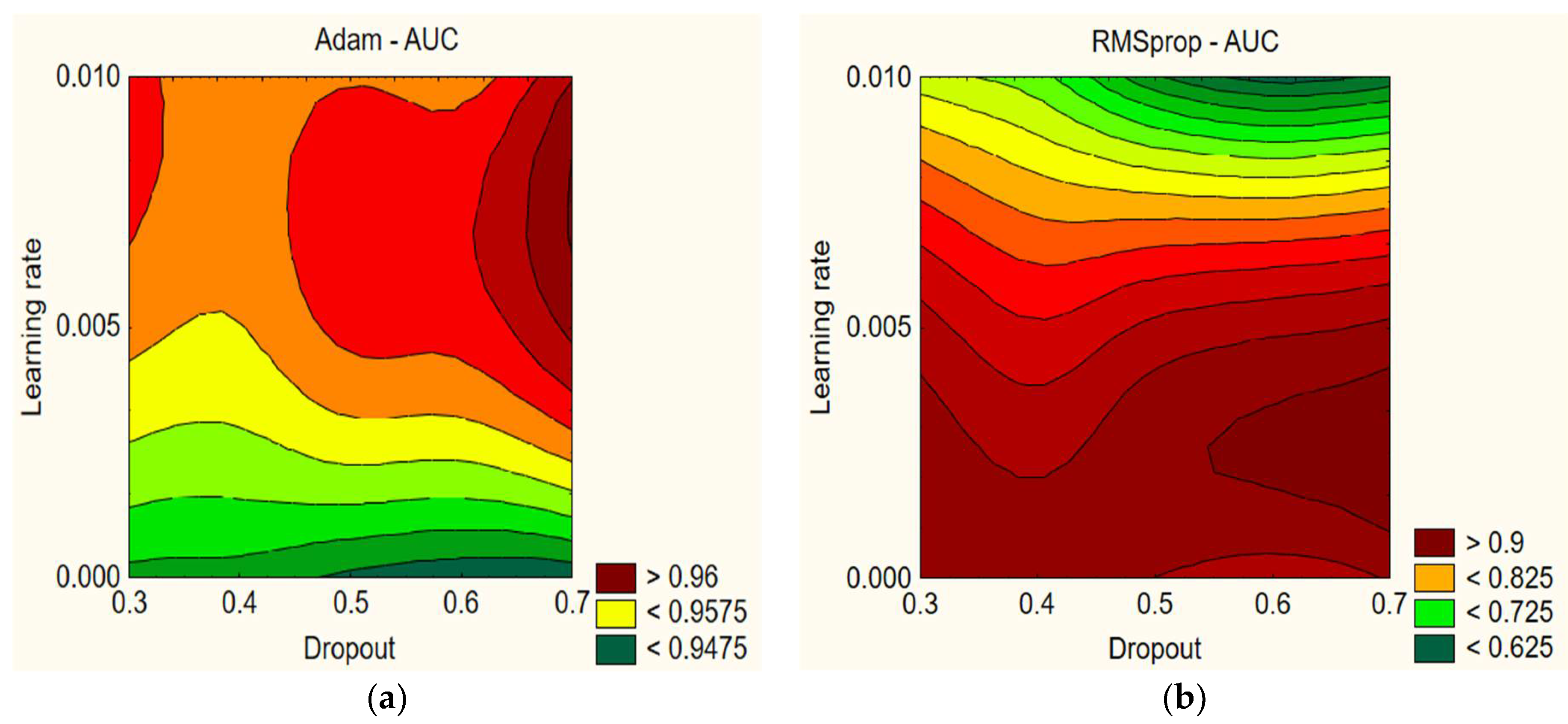
The effect of several model parameter combinations on AUC, accuracy, and F1 was compared for different optimizers. Figure 1, Figure 2 and Figure 3 compare the impact of dropout rate and learning rate.

In Figure 1, we can see that the AUC values are relatively high and range between 92.79% and 97.45% with the Adam optimizer. The AUC values slightly vary depending on the learning rate and dropout. Furthermore, it can be concluded that a model that uses a higher learning rate and dropout (for example, a learning rate of 0.005 and dropout of 0.7) can achieve a better AUC value. With the RMSprop optimizer, lower dropout percentages (0.3–0.4) and lower learning rates (0.001) tend to result in higher AUC values. On the other hand, combinations of higher dropout percentages (0.6–0.7) and higher learning rates (0.01) tend to result in lower AUC values, which may indicate that these combinations can cause too much fluctuation during training and hinder the model’s learning ability. Based on these findings, it can be concluded that selecting the appropriate learning rate and dropout percentage combination has a significant impact on the AUC variations. Properly selecting these parameters can improve the model’s performance and increase AUC values (see

Table 5. Key results on learning rate and dropout impact on AUC. LR—learning rate, d—dropout.

Optimizer	d	LR	g1 Accuracy	g2 Accuracy	Accuracy	AUC	Precision	Recall	F1
Adam	0.7	0.005	51.8731	88.6591	94.6000	97.4530	97.6644	95.2743	96.4545
Adam	0.6	0.01	53.0571	89.9248	91.8667	92.7979	94.6655	94.3460	94.5055
RMSProp	0.4	0.005	57.3184	86.6276	92.8667	96.8271	94.7631	96.2025	95.4774
RMSProp	0.4	0.01	54.4411	22.7191	21.0000	50.0000	0.0000	0.0000	0.0000

).

Using the Adam optimizer, the highest AUC is achieved with a learning rate of 0.005 and dropout of 0.7, resulting in an AUC of 97.45%, whereas the lowest AUC is achieved with a learning rate of 0.01 and dropout of 0.6, resulting in an AUC of 92.79%. With the RMSprop optimizer, the highest AUC is achieved with a learning rate of 0.005 and dropout of 0.4, resulting in an AUC of 96.82%, whereas the lowest AUC is achieved with a learning rate of 0.01 and dropout of 0.4, resulting in an AUC of 50%. Overall, the Adam optimizer shows better results on average.

In Figure 2, using the Adam optimizer, when the learning rate is 0.005 and dropout rate is 0.7, the model achieves the highest accuracy result (94.6%), whereas the lowest accuracy (87.73%) is obtained with a learning rate of 0.001 and dropout rate of 0.3. With RMSprop, the highest accuracy (93.8%) was achieved with a learning rate of 0.005 and dropout rate of 0.6, whereas the lowest accuracy (21%) was obtained with a learning rate of 0.01 and dropout rate of 0.7. Overall, all Adam optimizer results provide good results, whereas the RMSprop results are highly variable.

With the Adam optimizer, lower dropout rates generally result in better accuracy, whereas higher dropout rates (0.7) and lower learning rates (0.001) can decrease accuracy. Both learning rate and dropout rate have an impact on the model’s accuracy indicators. When analyzing the presented data with RMSprop, we can also see that different learning rates and dropout rates have varying effects on the model’s accuracy. For example, a network with a learning rate of 0.01 generally has poorer accuracy results (even up to 21%), whereas lower dropout rates tend to produce better accuracy (see

Table 6. Key results on learning rate and dropout impact on Accuracy. LR—learning rate, d—dropout.

Optimizer	d	LR	g1 Accuracy	g2 Accuracy	Accuracy	AUC	Precision	Recall	F1
Adam	0.7	0.005	51.8731	88.6591	94.6000	97.4530	97.6644	95.2743	96.4545
Adam	0.3	0.001	70.4137	82.2759	87.7333	94.4294	96.2072	87.7637	91.7917
RMSProp	0.6	0.005	54.3027	89.4659	93.8000	96.3909	94.8971	97.2996	96.0833
RMSProp	0.7	0.01	54.3165	22.9941	21.0000	50.0000	0.0000	0.0000	0.0000

).

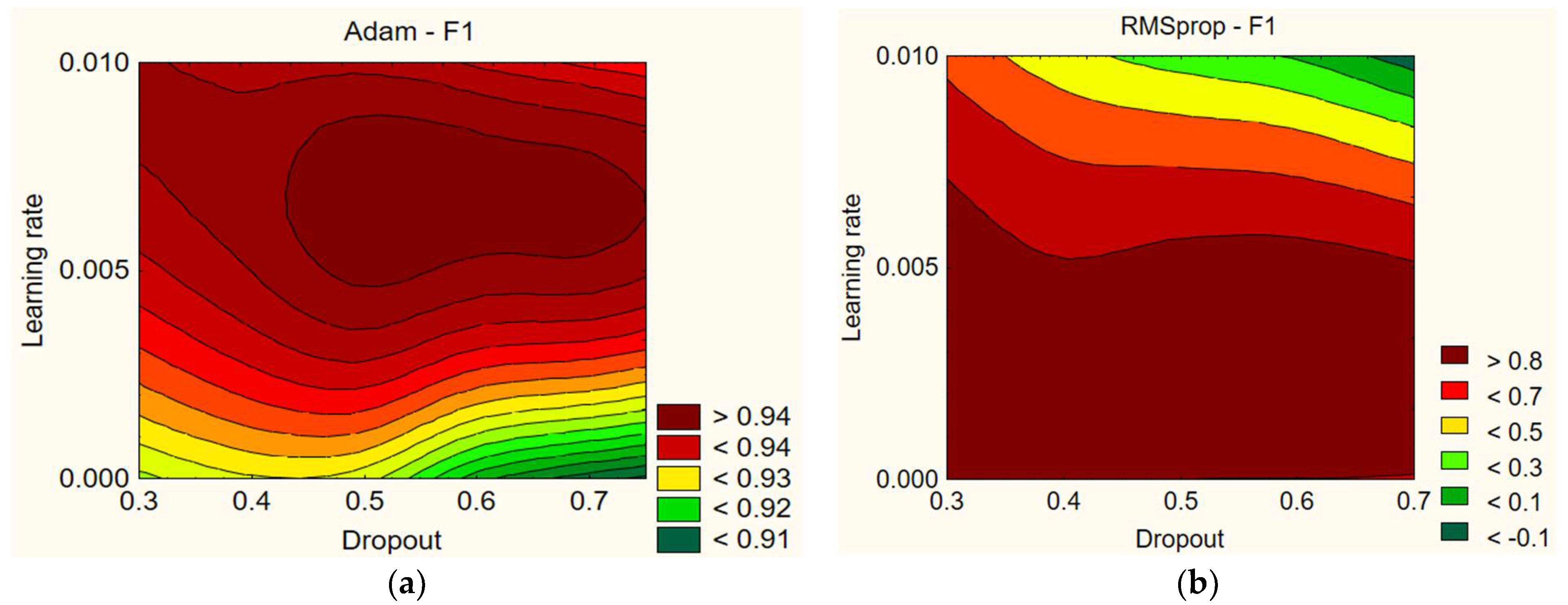
In Figure 3, the data show that different values of learning rate and dropout have a small effect on the F1 score. For example, with the Adam optimizer, using a dropout of 0.7 and a learning rate of 0.005 gives the highest F1 score of 96.45%. Meanwhile, with a dropout of 0.6 and a learning rate of 0.001, the F1 score decreases to 90.74%. Overall, the F1 scores for the Adam optimizer are sufficiently high, but the data show that it is difficult to say whether the learning rate and dropout have a certain influence on the F1 score. However, it can be noted that the F1 score is lower with lower learning rate values (0.001). The results with the RMSprop optimizer are highly variable. Using a dropout of 0.3 and a learning rate of 0.005 gives the highest F1 score of 96.14%. Meanwhile, with a dropout of 0.7 and a learning rate of 0.01, the F1 score drops to 0%. Overall, the F1 scores for the RMSprop optimizer are widely dispersed, but the data show that the learning rate and dropout have a certain influence on the F1 score. Lower dropout rates and lower learning rates lead to better results. Comparing Adam and RMSprop, higher learning rate values in both optimizers resulted in worse F1 scores (see

Table 7. Key results on learning rate and dropout impact on F1. LR—learning rate, d—dropout.

Optimizer	d	LR	g1 Accuracy	g2 Accuracy	Accuracy	AUC	Precision	Recall	F1
Adam	0.7	0.005	51.8731	88.6591	94.6000	97.4530	97.6644	95.2743	96.4545
Adam	0.6	0.001	68.1292	87.2029	91.4000	94.2254	97.5728	84.8101	90.7449
RMSProp	0.3	0.005	62.9173	88.4458	93.7333	96.3850	95.4281	96.8776	96.1474
RMSProp	0.7	0.01	54.3165	22.9941	21.0000	50.0000	0.0000	0.0000	0.0000

).

Figure 4, Figure 5 and Figure 6 compare the impact of block size and learning rate. In Figure 4, we can see from the Adam data that it can be observed that AUC values vary depending on the learning rate and the block size. It can also be concluded that a model that uses a smaller block size and a higher learning rate (for example, input length of 30–60 and learning rate of 0.005–0.01) can achieve a better AUC value. For instance, when the block size is 30 and the learning rate is 0.01, the AUC is 96.81%, whereas it decreases to 92.79% when the block size is 120, which is almost 4% lower. With RMSprop, it can be observed that combinations of shorter block sizes (30) and lower learning rates (0.001) tend to result in higher AUC values. Conversely, combinations of longer input lengths (120) and higher learning rates (0.01) result in lower AUC values (see

Table 8. Key results on learning rate and block size impact on AUC. LR—learning rate, BS—block size.

Optimizer	BS	LR	g1 Accuracy	g2 Accuracy	Accuracy	AUC	Precision	Recall	F1
Adam	30	0.01	52.8728	83.9425	89.4667	96.8176	98.2092	87.9325	92.7872
Adam	120	0.01	53.0571	89.9248	91.8667	92.7979	94.6655	94.3460	94.5055
RMSProp	30	0.001	74.3008	86.6768	92.6000	96.6964	92.9365	98.8186	95.7873
RMSProp	120	0.001	73.2480	84.6638	89.7333	93.6729	97.7473	84.2194	90.4805

).

For instance, with a block size of 30 and a learning rate of 0.001, the AUC is 96.69%. However, it decreases to 93.67% when the block size increases to 120. From these observations, we can conclude that an appropriate combination of learning rate and block size significantly influences the variation in the AUC.

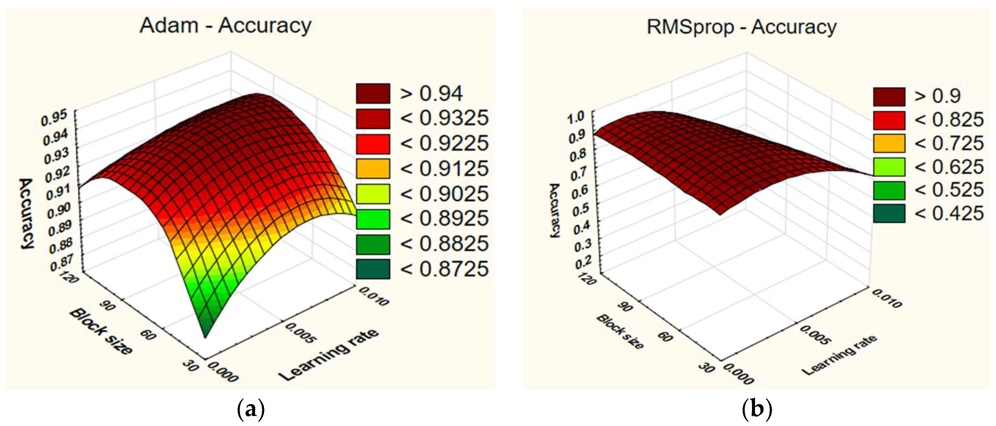
From Figure 5, it is evident that the highest accuracy (93.8%) was achieved with a learning rate of 0.005 and a block size of 60when using RMSprop. Conversely, the lowest accuracy (21%) was observed when using a learning rate of 0.01 across all block sizes (30, 60, and 120). When employing Adam, the highest accuracy result (94.6%) was obtained with a learning rate of 0.005 and a block size of 60. On the other hand, the lowest accuracy (87.33%) was achieved with a learning rate of 0.001 and a block size of 30.

The block size does not have a significant impact on the results when using the RMSprop optimizer. Generally, all block size options yield similar performance, but slightly worse results are observed with a block size of 120. For instance, a network with a learning rate of 0.001 and a block size of 120 achieves an accuracy of 90.4%. With a block size of 30, the accuracy is 91%, and the accuracy is 92% with a block size of 60. On the other hand, the learning rate does have an impact, with poorer results observed when using a learning rate of 0.01. With the Adam optimizer, it can be observed that the learning rate has a lesser impact on the results. The results across different learning rates are relatively similar. However, the block size has a more pronounced effect. The best results are obtained with a block size of 60, whereas the worst results are observed with a block size of 30. The results for a block size of 120 fall approximately in the middle. For example, a network with a block size of 60 achieves an accuracy of 92.4%, whereas the accuracy is 89.46% with a block size of 30. With a block size of 120, the accuracy is 91.86% (see

Table 9. Key results on learning rate and block size impact on accuracy. LR—learning rate, BS—block size.

Optimizer	BS	LR	g1 Accuracy	g2 Accuracy	Accuracy	AUC	Precision	Recall	F1
Adam	60	0.005	51.8731	88.6591	94.6000	97.4530	97.6644	95.2743	96.4545
Adam	30	0.001	70.4137	82.2759	87.7333	94.4294	96.2072	87.7637	91.7917
Adam	30	0.01	52.8728	83.9425	89.4667	96.8176	98.2092	87.9325	92.7872
Adam	60	0.01	53.2641	88.5757	92.4000	96.8222	98.0961	91.3080	94.5804
Adam	120	0.01	53.0571	89.9248	91.8667	92.7979	94.6655	94.3460	94.5055
RMSProp	60	0.005	54.3027	89.4659	93.8000	96.3909	94.8971	97.2996	96.0833
RMSProp	120	0.01	54.3165	22.9941	21.0000	50.0000	0.0000	0.0000	0.0000
RMSProp	30	0.001	72.9247	85.8949	91.0000	94.7229	92.2705	96.7089	94.4376
RMSProp	60	0.001	75.9366	87.5371	92.0000	94.3806	93.9819	96.2025	95.0792
RMSProp	120	0.001	70.9933	87.7717	90.4000	91.7142	95.3971	89.1983	92.1936

).

Observations with the Adam optimizer (refer to Figure 6) indicate that the choice of block size and learning rate significantly influences the F1 score. Generally, increasing the block size from 30 to 60 results in an enhancement in the F1 score. However, further increases up to 120 do not consistently yield positive effects on the F1 score. This behavior might be attributed to the larger block size, facilitating the model’s understanding of longer contexts, but excessively large block sizes could adversely affect training due to the increased complexity and memory requirements. Regarding the learning rate, the F1 scores’ distribution is quite diverse, suggesting that the learning rate does not have a significant influence. In contrast, with RMSprop, we observe that the learning rate has a more pronounced impact compared to the block size. A learning rate of 0.01 yields the poorest results, whereas both 0.005 and 0.001 provide better outcomes. In terms of recording length, optimal results are typically achieved with a block size of 60. However, satisfactory results can also be achieved with block sizes of 30 and 120, although the latter yields comparatively poorer average results. The impact of learning rate and block size on the F1 score is detailed in

Table 10. Key results on learning rate and block size impact on F1. LR—learning rate, BS—block size.

Optimizer	BS	LR	g1 Accuracy	g2 Accuracy	Accuracy	AUC	Precision	Recall	F1
Adam	120	0.005	48.2023	89.7623	92.2000	95.5069	97.0988	90.3797	93.6189
Adam	60	0.005	51.8731	88.6591	94.6000	97.4530	97.6644	95.2743	96.4545
Adam	30	0.005	48.5479	85.1622	91.4667	97.1134	97.8102	90.4641	93.9939
RMSProp	120	0.001	70.9933	87.7717	90.4000	91.7142	95.3971	89.1983	92.1936
RMSProp	60	0.005	54.6643	89.3268	93.2000	95.9257	94.6590	97.2152	95.9201
RMSProp	30	0.01	54.4411	22.7191	21.0000	50.0000	0.0000	0.0000	0.0000

. Figure 7, Figure 8 and Figure 9 compare the impact of block size and learning rate.

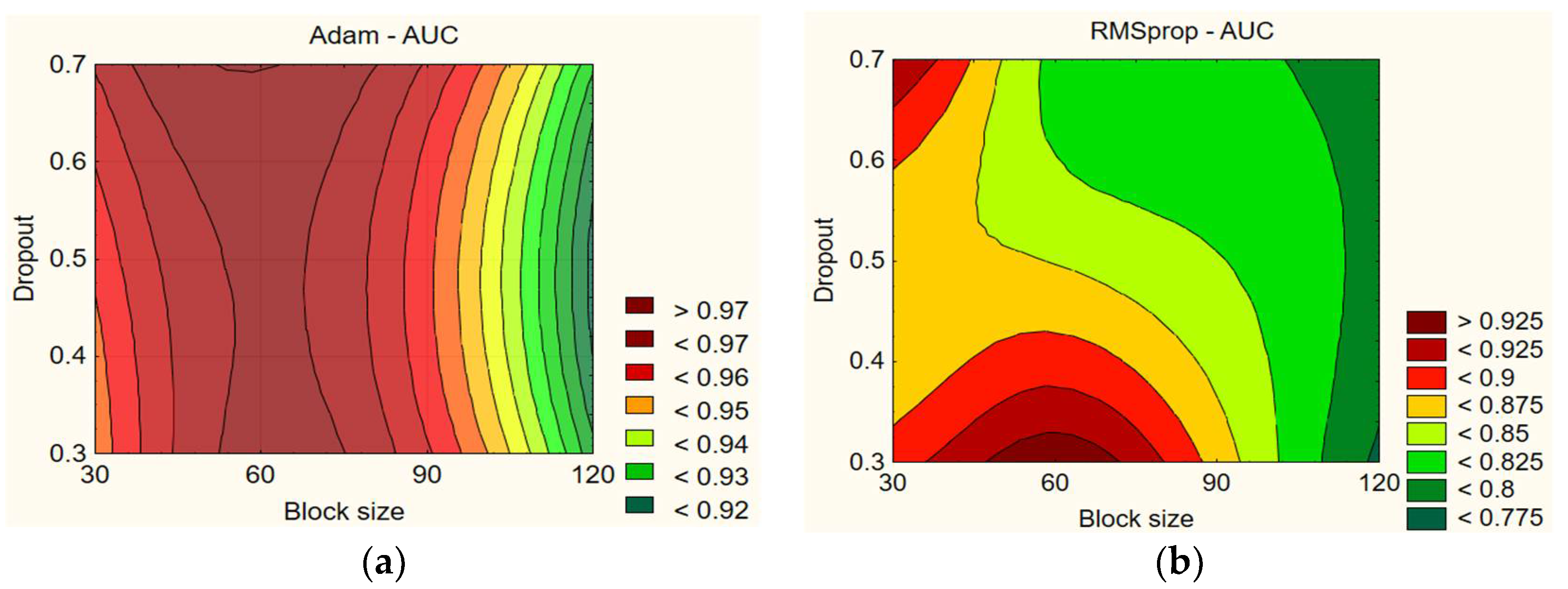
In Figure 7, when examining the data for Adam, it can be noticed that higher dropout (0.6–0.7) with a block size of 60 generally leads to higher AUC values. For example, with a dropout of 0.7 and a block size of 60, the AUC reaches 97.45%, and it is 97.29% with a dropout of 0.6. However, worse AUC values are obtained with longer block sizes. For example, with a dropout of 0.7 and a block size of 120, the AUC is 95.51%, whereas it is 93.91% with a dropout of 0.6. When the dropout is lower (0.3–0.4), worse results are obtained. For example, with a block size of 30 and a dropout of 0.7, the AUC is 97.11%, whereas it is 95.93% with a dropout of 0.3. With RMSprop, lower AUC values are obtained with a block size of 120, whereas it depends on the dropout with other block size combinations. For example, with a dropout of 0.3 and a block size of 60, the AUC reaches 96.38%, whereas it is 95.39% with a dropout of 0.7 and a block size of 30. The highest values are obtained with a block size of 60 and a low dropout or with a smaller block size of 30 and a higher dropout (0.6–0.7). The results on dropout and block size impact on AUC are presented in

Table 11. Key results on dropout and block size impact on AUC. D—dropout, BS—block size.

Optimizer	BS	d	g1 Accuracy	g2 Accuracy	Accuracy	AUC	Precision	Recall	F1
Adam	60	0.7	51.8731	88.6591	94.6000	97.4530	97.6644	95.2743	96.4545
Adam	60	0.6	54.2378	89.1970	93.4000	97.2923	96.8158	94.9367	95.8671
Adam	120	0.7	48.2023	89.7623	92.2000	95.5069	97.0988	90.3797	93.6189
Adam	120	0.6	54.3165	88.7264	91.0667	93.9176	96.3669	89.5359	92.8259
Adam	30	0.7	48.5479	85.1622	91.4667	97.1134	97.8102	90.4641	93.9939
Adam	30	0.3	53.3554	84.7824	89.1333	95.9313	95.1370	90.8017	92.9188
RMSProp	60	0.3	62.9173	88.4458	93.7333	96.3850	95.4281	96.8776	96.1474
RMSProp	30	0.7	54.6198	87.0119	91.2000	95.3986	92.1900	96.6245	94.3552

.

In Figure 8, the data for the Adam optimizer reveals that the dropout rate has a lesser impact compared to the block size. Generally, higher accuracy values are achieved with a block size of 60. For instance, with a dropout rate of 0.7 and a block size of 60, the accuracy reaches 94.6%. Conversely, with different block sizes, lower accuracy values are observed. For example, with a dropout rate of 0.7 and a block size of 120, the accuracy reaches 92.2%, whereas it is 89.13% with a dropout rate of 0.3 and a block size of 30. With RMSprop, the dropout rate also has a lesser impact compared to the block size. However, better accuracy is obtained with smaller block sizes, specifically in the range of 30–60. For instance, with a dropout rate of 0.3 and a block size of 60, the accuracy reaches 93.73%, whereas it is 86.46% with a block size of 120. However, with a dropout rate of 0.7 and a block size of 120, the accuracy improves to 90.6%. Results are presented in

Table 12. Key results on dropout and block size impact on accuracy. D—dropout, BS—block size.

Optimizer	BS	d	g1 Accuracy	g2 Accuracy	Accuracy	AUC	Precision	Recall	F1
Adam	60	0.7	51.8731	88.6591	94.6000	97.4530	97.6644	95.2743	96.4545
Adam	60	0.3	53.7927	88.3717	93.0667	96.6929	96.9244	93.0802	94.9634
Adam	120	0.7	48.2023	89.7623	92.2000	95.5069	97.0988	90.3797	93.6189
Adam	30	0.3	53.3554	84.7824	89.1333	95.9313	95.1370	90.8017	92.9188
RMSProp	60	0.3	62.9173	88.4458	93.7333	96.3850	95.4281	96.8776	96.1474
RMSProp	120	0.3	54.3165	87.3248	86.4667	85.1542	92.2399	88.2700	90.2113
RMSProp	120	0.7	54.2555	89.0108	90.6000	92.7190	95.2756	91.8987	93.5567

.

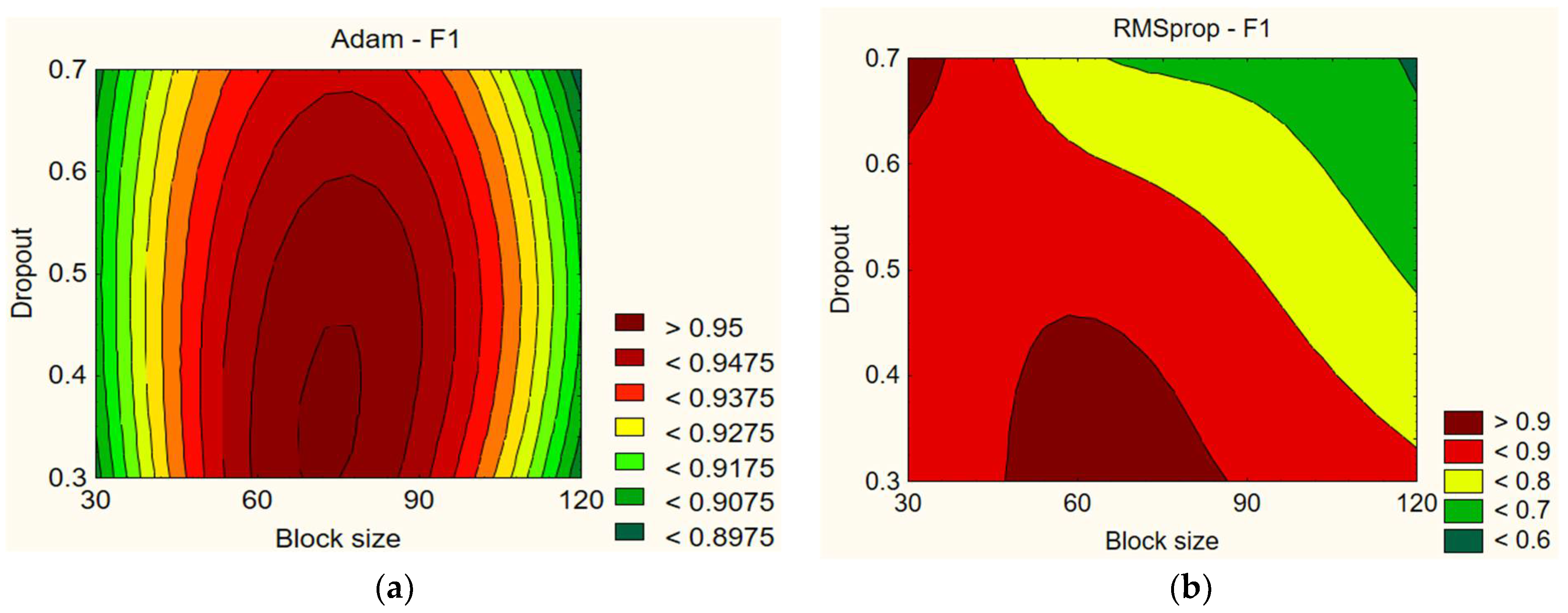
In Figure 9, the data demonstrate that different values of block sizes and dropout have an impact on the F1 score. When using the Adam optimizer, lower dropout values (e.g., 0.3 and 0.4) result in higher F1 scores compared to higher dropout values (e.g., 0.6 and 0.7), and both 30 and 120 block sizes lead to worse results. For instance, the F1 score is 92.14% using a dropout of 0.7 and a block size of 30, and it is 90.81% for a block size of 120. However, with a dropout of 0.3 and a block size of 60, the F1 score improves to 95.51%. Overall, the results from the Adam optimizer indicate that dropout and block size have an impact on the F1 score (see

Table 13. Key results on dropout and block size impact on F1. D—dropout, BS—block size.

Optimizer	BS	d	g1 Accuracy	g2 Accuracy	Accuracy	AUC	Precision	Recall	F1
Adam	30	0.7	71.1688	83.1874	88.8000	95.8642	97.1910	87.5949	92.1438
Adam	120	0.7	48.2023	74.2230	90.0667	93.0309	96.8451	85.4852	90.8113
Adam	60	0.3	72.1254	87.8709	93.7333	96.9391	96.6321	94.4304	95.5186
RMSProp	60	0.3	62.9173	88.4458	93.7333	96.3850	95.4281	96.8776	96.1474
RMSProp	30	0.7	77.7455	85.9262	92.2667	95.6827	93.6637	97.2996	95.4470
RMSProp	120	0.7	54.4587	86.0045	89.0000	91.8000	96.7086	84.3038	90.0812

).

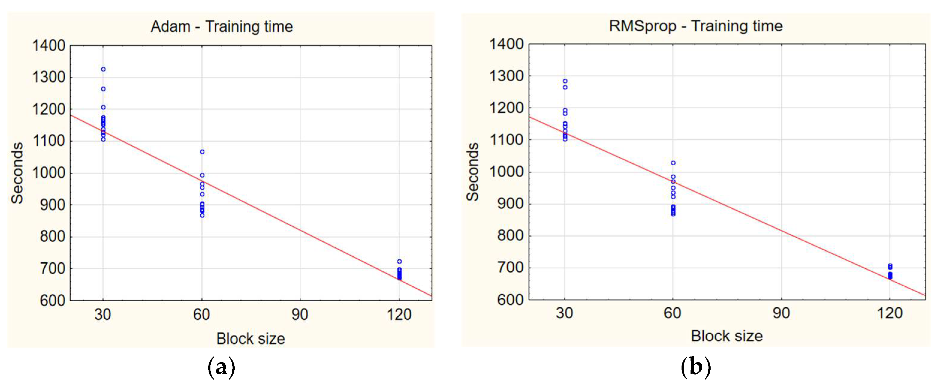
With the RMSprop optimizer, the results show slight differences. Significantly worse results are observed only with a block size of 120, whereas similar results are obtained with other parameter combinations. The best result is achieved with a dropout of 0.3 and a block size of 60, yielding an F1 score of 96.14%. Using a dropout of 0.7 and a block size of 30, the F1 score is 95.44%. However, when using a dropout of 0.7 and a block size of 120, the F1 score drops to 90.08%. Overall, the data from RMSprop demonstrate that dropout and block size impact the F1 score. When comparing Adam and RMSprop, the F1 scores are very similar, but the scores obtained with the Adam optimizer are slightly higher. Figure 10 compares the training times based on different block sizes.

Firstly, a larger block size of 120 generally results in shorter training times compared to smaller block sizes of 30 and 60. This can be explained by the fact that a larger block size provides more efficient data utilization, reducing the number of updates per epoch. To better understand the relationship between time and block size, it is worth reviewing some average times by block size:

• Block size 30: about 1100 s;
• Block size 60: about 900 s;
• Block size 120: about 700 s.

From these results, we see that increasing the record length from 30 to 120 reduces the average training time by about 37%. However, it is important to note that although a larger block size can help reduce training time, it affects the accuracy of the model.

Summarized results of the experiment are provided in

Table 14. Comparison of reported, reproduced, and best results of Adam and RMSprop in the experiment with c23 dataset.

Optimizer—Parameter	g1 Accuracy	g2 Accuracy	Accuracy	AUC	Precision	Recall	F1
Reproduced results	63.5756	87.1847	92.9333	96.8073	96.7629	93.3333	95.0171
Reported results	-	-	-	97.3	-	-	-
Adam—best experiment results	51.8731	88.6591	94.6	97.453	97.6644	95.2743	96.4545
RMSprop—best experiment results	57.3184	86.6276	92.8667	96.8271	94.7631	96.2025	95.4774

.

The initial reproduced data exhibit quite high results, especially the accuracy of g1—63.58%, the highest of all other models, and other results: g2 accuracy—87.18%; overall accuracy—92.93%; AUC—96.80%; Precision—96.76%; Recall—93.33%; and F1—95.02%. The article provided limited information on the c23 data level, but the AUC is very high—97.3%. The research results with Adam achieve the highest results among all models, in almost all criteria, except for g1—51.87% and Recall—95.27%. Furthermore, g2 accuracy—88.66%; overall accuracy—97.45%; AUC—97.45%; Precision—97.66%; Recall—95.27%; and F1—96.45%. RMSprop with the best parameters also exhibits high indicators, but overall has inferior results compared to the research results of Adam: g1 accuracy—57.31%; g2 accuracy—86.62%; overall accuracy—92.86%; AUC—96.82%; Precision—94.76%; Recall—96.20%; and F1—95.47%.

The main parameters are overall accuracy, AUC, and F1, and, during the research, the best results with the Adam optimizer surpass the AUC results indicated in the article by 0.1%. Compared to the reproduced model results, AUC is improved by 0.6%. Additionally, compared to the reproduced model results, g2 is improved by 1.5%, overall accuracy by 1.7%, and F1 by 1.4%. However, when comparing the reproduced model results with the best RMSprop research results, RMSprop results are slightly inferior or almost identical, except for the F1 result, which is better by 0.4%.

Based on this analysis, the best Adam research results indicate that there are parameters for this model that produce better results, and these parameters are selected for further analysis because they exhibit the highest results in almost all measurement indicators. These best parameters are:

• Learning rate—0.005;
• Dropout rate—0.7;
• Sequence length—60;
• Optimizer—Adam.

Therefore, by choosing these new parameters, the model is trained using previous training data, but with 5-fold cross-validation to further verify that the training is consistently better than the results reported in the article. The testing data are left the same as specified in the article. The cross-validation training results of the model are shown in

Table 15. Comparison of reported, reproduced, and Adam with the best parameters found in the experiment with all dataset levels.

Dataset Level	g1 Accuracy	g2 Accuracy	Accuracy	AUC	Precision	Recall	F1
Reproduced—“raw”	86.3806	91.7724	95.7143	97.8705	96.9965	98.0357	97.5133
Reproduced—“c23”	63.5757	87.1847	92.9333	96.8073	96.7629	93.3333	95.0172
Reproduced—“c40”	81.5299	82.444	91.2857	93.7111	93.5315	95.5357	94.523
Reported—“raw”	83.4	98.3	99.7	99.9	-	-	-
Reported—“c23”	-	-	-	97.3	-	-	-
Reported—“c40”	80.4	85.2	91.2	95.7	-	-	-
Best parameters—“raw”	21.7164	90.5671	95.3142	97.4330	96.7902	97.9285	97.3553
Best parameters—“c23”	21.7164	91.5485	96.4285	98.0241	97.4188	98.1428	97.7770
Best parameters—“c40”	32.6412	82.9144	89.6571	90.6779	90.8831	97.25	93.9395

.

In this table, the reproduced results of the article, the results reported in the article, and the average results obtained by performing a 5-fold cross-validation with the best parameters found during the experiment are presented. The best parameters’ “raw” results show a g1 accuracy of 21.71%, a g2 accuracy of 90.56%, an overall accuracy of 95.31%, an AUC of 97.43%, a precision of 96.79%, a recall of 97.93%, and an F1 score of 97.36%. The results show that none of the parameters are improved compared to the reproduced or reported results with these parameters and “raw” dataset. Compared to the reported results, the accuracy is about 5% lower, and the AUC is about 2% lower, with g1 being completely poor and practically not working correctly. With the “c23” dataset, the results show a g1 accuracy of 21.71%, a g2 accuracy of 91.54%, an overall accuracy of 96.43%, an AUC of 98.02%, a precision of 97.42%, a recall of 98.14%, and an F1 score of 97.78%. Compared to the AUC result reported in the article, it was improved by 0.7%, and the other results were not reported in the article for this dataset level. Compared to the reproduced model results, all results are improved except for g1. The accuracy is improved by 3.5%, the AUC by 1.2%, and the F1 score by 2.7%. Finally, with the “c40” dataset, the results show a g1 accuracy of 32.64%, a g2 accuracy of 82.91%, an overall accuracy of 89.66%, an AUC of 90.68%, a precision of 90.88%, a recall of 97.25%, and an F1 score of 93.94%. Compared to the “c40” results reported in the article, all results are slightly lower by a few percentage points, e.g., the accuracy is 1.7% lower, and the AUC is 5% lower. Compared to the reproduced model results, the accuracy and AUC results are still lower, but the g1 accuracy is 0.5% better, and the recall is 1.7% better. In summary, this new model results in slightly improved “c23” AUC results.

To verify that the results obtained with the new parameters are consistent, the standard deviations and variation coefficients of the cross-validation results are presented in

Table 16. Best model parameter model cross-validation standard deviation and variation coefficient results.

Dataset Level	g1 Accuracy	g2 Accuracy	Accuracy	AUC	Precision	Recall	F1
“raw”—standard deviation	0	0.0058	0.0064	0.0042	0.0052	0.0027	0.0029
“raw”—variation coefficient	0	0.6510	0.6819	0.4331	0.5469	0.2765	0.2996
“c23”—standard deviation	0	0.0015	0.0050	0.0029	0.0076	0.0044	0.0030
“c23”—variation coefficient	0	0.1698	0.5237	0.2966	0.7877	0.4566	0.3078
“c40”—standard deviation	74.8396	2.2038	2.8382	3.7282	2.6524	1.3405	1.3780
“c40”—variation coefficient	32.6412	82.9144	89.6571	90.6779	90.8831	97.25	93.9395

.

When comparing the standard deviations of different data sets, the “raw” data set has larger standard deviation sizes for g2 accuracy, overall accuracy, and AUC compared to the “c23” data set. The “c40” data set has larger standard deviation sizes for all parameters compared to the “raw” and “c23” data sets, except for g1 accuracy, whose standard deviation is equal to 0. However, overall, the standard deviations are low for all data sets. Comparing the variation coefficient of different data sets, the “raw” data set has larger coefficient of variation sizes for g2 accuracy, overall accuracy, AUC, precision, and recall, compared to the “c23” data set. The “c40” data set has a significantly larger variation coefficient for g1 accuracy compared to other models, as well as larger variation coefficient sizes for all other parameters compared to the “raw” and “c23” models. The AUC standard deviation of the “c23” data set results (0.0050) is smaller than the standard deviations of the “raw” (0.0064) and “c40” (0.0254) models. A smaller standard deviation indicates that the “c23” AUC results are more concentrated around the mean, and, therefore, the model is more stable and has less result dispersion. In addition, the “c23” data set AUC variation coefficient (0.5237) is smaller than the variation coefficients for the “raw” (0.6819) and “c40” (2.8382) data sets. A smaller variation coefficient indicates that the “c23” AUC results are less dispersed compared to the results of other data sets.

Based on these comparisons, we can conclude that the model is more efficient and more stable when it comes to AUC results with the “c23” data set, and these results effectively improve the AUC results reported in the article.

4.2. Improved Model

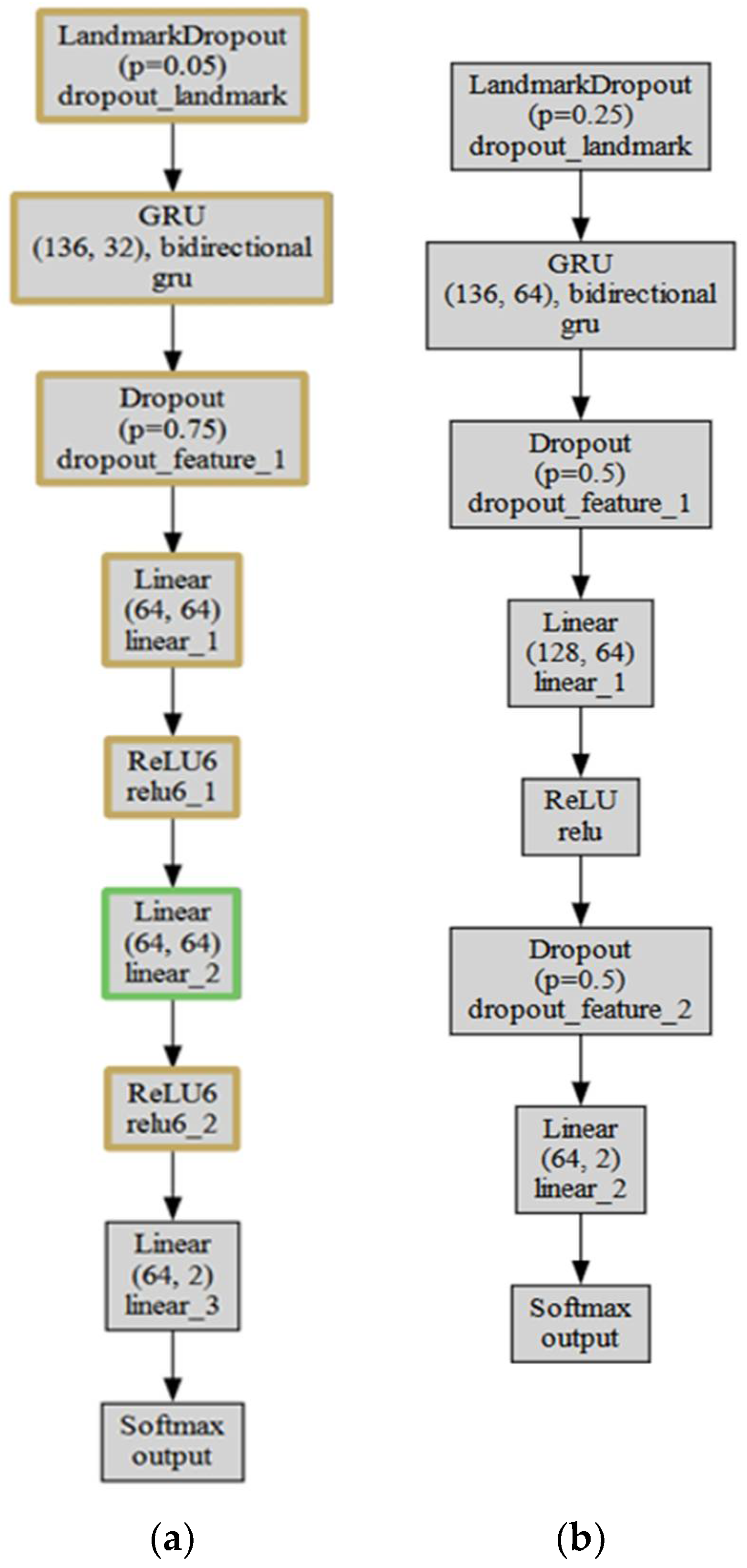
Based on the results obtained in the previous section, a new improved model version is presented in Figure 11. When creating this model, the goal was to improve the AUC results and accuracy for the “c23” data level, compared to the results reported in the article or during the experiment. The “c23” data level is also important because these data are subject to data compression, which is often encountered on the internet; thus, this data could be more important considering the relevance of the models’ usage. AUC and accuracy are the most important indicators of model effectiveness in distinguishing true images from fake ones.

The main differences between the two models are the first dropout rate, the number of GRU hidden neurons, the number of dropout layers, and the configuration of linear layers and activation functions. The improved model has a smaller number of GRU hidden neurons and additional linear and ReLU6 layers, whereas LRNet has a higher first dropout rate and one additional dropout layer.

When comparing the two models, the improved model and LRNet, several key differences in their structure are observed. First, the improved model uses a smaller first dropout rate—0.05—compared to LRNet’s of 0.25. Second, the GRU hidden neuron count is smaller in the improved model—32—compared to LRNet’s 64. In addition, the improved model has one dropout layer with a 0.75 dropout rate, whereas LRNet has two dropout layers with a 0.5 dropout rate. The configuration of linear layers and activation functions is also different. The improved model has three linear layers with ReLU6 activation functions, whereas LRNet has two linear layers with ReLU activation functions. Additionally, the number of neurons in the linear layers of the improved model is smaller since the output of the GRU layer is smaller. The linear layers of the improved model are: 64 × 64, 64 × 64, 64 × 2, whereas LRNet has 128 × 64, 64 × 2. Finally, both models have a Softmax output layer with a single output. The improved model is more complex, with additional linear layers and ReLU6 activation functions, whereas LRNet has a higher first dropout layer coefficient and one additional dropout layer.

The model was trained using previous training data but with 5-fold cross-validation to further verify training errors and ensure that the model consistently achieved better results. However, the testing data remained the same as reported in the article. The cross-validation results for the improved model are shown in

Table 17. Comparison between different models.

Dataset Level	g1 Accuracy	g2 Accuracy	Accuracy	AUC	Precision	Recall	F1
Reproduced—“raw”	86.3806	91.7724	95.7143	97.8705	96.9965	98.0357	97.5133
Reproduced—“c23”	63.5757	87.1847	92.9333	96.8073	96.7629	93.3333	95.0172
Reproduced—“c40”	81.5299	82.444	91.2857	93.7111	93.5315	95.5357	94.523
Reported—“raw”	83.4	98.3	99.7	99.9	-	-	-
Reported—“c23”	-	-	-	97.3	-	-	-
Reported—“c40”	80.4	85.2	91.2	95.7	-	-	-
Best parameters—“raw”	21.7164	90.5671	95.3142	97.4330	96.7902	97.9285	97.3553
Best parameters—“c23”	21.7164	91.5485	96.4285	98.0241	97.4188	98.1428	97.7770
Best parameters—“c40”	32.6412	82.9144	89.6571	90.6779	90.8831	97.25	93.9395
Improved model—“raw”	79.7798	90.7014	94.5428	96.9191	95.9633	98.1071	97.0193
Improved model—“c23”	77.7686	92.4029	96.1714	98.3896	96.7534	98.7142	97.7213
Improved model—“c40”	76.7089	83.4552	88.5428	89.1908	89.142	98.2857	93.4827

.

This table presents the reproduced results, reported results, the average of the results obtained from the cross-validation with the best parameters found during the experiment, and the average of the results obtained from the cross-validation with the improved model. The improved model’s “raw” variant achieved very similar results to the reproduced model’s “raw” and the best parameter model’s “raw” results. This indicated that the improved model with the “raw” dataset had slightly lower performance indicators, such as g1 accuracy (79.78%), g2 accuracy (90.70%), overall accuracy (94.54%), AUC (96.92%), precision (95.96%), recall (98.11%), and F1 (97.02%). Compared to the reproduced model, AUC was 1% lower, with the reported model AUC 3% lower, and with the best parameter model AUC 0.5% lower. Secondly, the improved model’s “c23” variant achieved better results than the reproduced model in almost all criteria. g1 accuracy increased from 63.58% to 77.77%, g2 accuracy increased from 87.18% to 92.40%, overall accuracy increased from 92.93% to 96.17%, AUC increased from 96.80% to 98.39%, precision did not change, recall increased from 93.33% to 98.71%, and F1 increased from 95.01% to 97.72%. Compared with the data reported in the article, AUC improved by 1.08%, compared to the best parameter model by 0.36%, and compared to the reproduced model by 1.58%. Finally, the improved model’s “c40” variant showed similar results to the reproduced model. g1 accuracy decreased from 81.53% to 76.71%, but g2 accuracy increased from 82.44% to 83.46%, overall accuracy decreased from 91.28% to 88.54%, AUC decreased from 93.71% to 89.19%, precision decreased from 93.53% to 89.14%, recall increased from 95.53% to 98.29%, and F1 decreased from 94.52% to 93.48%. Compared to the best parameter model, almost all results were about 1% lower. In summary, the improved model showed the best AUC results with the “c23” dataset among all models and the best results for other parameters but showed slightly lower results with other datasets.

To ensure or verify that the results obtained with the improved model were consistent,

Table 18. Improved model stability data, based on standard deviations and variation coefficients.

Dataset Level	g1 Accuracy	g2 Accuracy	Accuracy	AUC	Precision	Recall	F1
“raw”—standard deviation	0.0113	0.0023	0.0077	0.0102	0.0129	0.0009	0.0062
“raw”—variation coefficient	1.4258	0.2596	0.823	1.0610	1.3523	0.099	0.6465
“c23”—standard deviation	0.0291	0.0029	0.0079	0.0049	0.0093	0.0029	0.0040
“c23”—variation coefficient	3.7488	0.3164	0.8230	0.5056	0.9692	0.2972	0.4178
“c40”—standard deviation	0.0483	0.0073	0.0156	0.0316	0.0148	0.0081	0.0076
“c40”—variation coefficient	6.3069	0.8753	1.772	3.5487	1.6709	0.8286	0.8144

presents the standard deviations and variation coefficients of the cross-validation results.

When comparing the standard deviations of different datasets, the “raw” dataset exhibits smaller standard deviation sizes for g2 accuracy, overall accuracy, AUC, and F1, in comparison to the “c40” dataset. It also demonstrates smaller standard deviations for g2 and overall accuracy when compared to the “c23” dataset, albeit with a negligible difference. Conversely, the “c40” dataset displays larger standard deviation sizes for all parameters when compared to the “raw” and “c23” datasets. Overall, the standard deviations are minimal for all datasets, but the noteworthy finding is that the AUC and F1 standard deviations are the smallest with the “c23” dataset.

Regarding the coefficient of variation in different datasets, it was observed that the “c40” dataset exhibits larger coefficients of variation for g1 and g2 accuracy, overall accuracy, AUC, precision, recall, and F1 when compared to the “c23” and “raw” datasets. The “raw” dataset demonstrates the smallest coefficients of variation, except for AUC, precision, and F1 results. The “c23” dataset showcases the best AUC, precision, and F1 results.

The AUC standard deviation (0.0049) of the “c23” dataset is smaller than the standard deviations of the “raw” (0.0102) and “c40” (0.0316) datasets. A smaller standard deviation indicates that the AUC results of the “c23” dataset are more concentrated around the mean, suggesting a higher level of stability and reduced result variability for the model. Furthermore, the AUC variation coefficient (0.5056) of the “c23” dataset is smaller than the variation coefficients of the “raw” (1.0610) and “c40” (3.5487) datasets. A smaller variation coefficient indicates that the AUC results of the “c23” dataset are less dispersed in comparison to the results of the other datasets.

From these comparisons, it can be concluded that the model is more effective and operates more stable than with other datasets with the “c23” dataset, especially when it comes to AUC. This indicates that the enhanced model consistently improves upon the performance of the original model, enabling the better identification of manipulated images from real ones. Moreover, the overall accuracy of the improved model was enhanced compared to the results of the replicated model. Unfortunately, with other datasets and model parameters, the model did not achieve better results.

Overall, with the improved model and the best parameters found in our experiment, the analyses of the “c23”, “raw”, and “c40” datasets indicate that the model performs most optimally and stably with the “c23” dataset, particularly regarding the AUC measure. With this dataset, the model’s effectiveness in discerning real images from forged ones and its overall accuracy is improved. However, the model’s performance does not show similar improvements with other datasets and parameters. Comparing standard deviations and coefficients of variation, the “c23” dataset consistently exhibits less dispersion and variation in results, underlining its stability and efficiency. In contrast, the “raw” and “c40” datasets showed larger standard deviations and coefficients of variation for most parameters, highlighting their relatively less stable and consistent performance. The improvements we observed in the model’s accuracy for the “c23” dataset are a direct result of the specific optimizations we made, which were tailored based on the characteristics and patterns identified during our experimentation phase. However, it’s important to note that these optimizations were not necessarily designed to enhance performance on other datasets, such as the raw and “c40” datasets. This explains why the accuracy values for these datasets did not show similar improvements. The optimizations that improved performance for the “c23” dataset may not be effective for other datasets due to their unique characteristics and data composition. Consequently, the improvements significantly contributed to enhancing the model’s performance and stability, particularly in relation to AUC results.

5. Conclusions

This comprehensive study involved a review of scientific literature on deepfake detection methods, leading to the identification of 11 distinct detection techniques. These methods could be broadly classified into three categories: those analyzing video changes over time, those focused on facial areas, and other detection techniques, with most boasting a recognition accuracy of at least 90% for manipulated images. The study specifically focused on the deepfake detection technique put forth by Sun et al. [8], notable for its superior accuracy; this method detected video changes over time to spot fake videos. In a bid to enhance the outcomes presented in the scientific literature, the study included an in-depth examination of the model, tweaking various parameters such as block size, dropout rate, learning rate, and the optimizer. After a comprehensive review of 135 results, it was discovered that a learning rate of 0.005, a dropout rate of 0.7, a block size of 60, and the Adam optimizer yielded superior AUC results. The study concluded with the proposal of an enhanced method for deepfake detection, modifying the first layer’s Dropout coefficient, the number of GRU hidden neurons, the number of Dropout layers, and substituting the linear layers and activation function with ReLU6. This improved model surpassed both the AUC results detailed in Sun et al. [8] and those found with the best parameters identified in our experiment. Future work would involve testing with different datasets, comparing them, and identifying factors that affect the precision.

References

1. Kietzmann, J.; Lee, L.W.; McCarthy, I.P.; Kietzmann, T.C. Deepfakes: Trick or treat? Bus. Horiz. 2020, 63, 135–146. [Google Scholar] [CrossRef]
2. Vaccari, C.; Chadwick, A. Deepfakes and Disinformation: Exploring the Impact of Synthetic Political Video on Deception, Uncertainty, and Trust in News. Soc. Media Soc. 2020, 6, 1–13. [Google Scholar] [CrossRef] [Green Version]
3. Rössler, A.; Cozzolino, D.; Verdoliva, L.; Riess, C.; Thies, J.; Nießner, M. FaceForensics: A large-scale video dataset for forgery detection in human faces. arXiv 2018, arXiv:1803.09179. [Google Scholar]
4. Touvron, H.; Cord, M.; Douze, M.; Massa, F.; Sablayrolles, A.; Jégou, H. Training data-efficient image transformers & distillation through attention. arXiv 2021, arXiv:2012.12877. [Google Scholar]
5. Heo, Y.J.; Yeo, W.H.; Kim, B.G. DeepFake detection algorithm based on improved vision transformer. Appl. Intell. 2023, 53, 7512–7527. [Google Scholar] [CrossRef]
6. Zhao, H.; Zhou, W.; Chen, D.; Wei, T.; Zhang, W.; Yu, N. Multi-attentional Deepfake Detection. arXiv 2021, arXiv:2103.02406v3. [Google Scholar]
7. Seow, J.W.; Lim, M.K.; Phan, R.C.W.; Liu, J.K. A comprehensive overview of Deepfake: Generation, detection, datasets, and opportunities. Neurocomputing 2022, 513, 351–371. [Google Scholar] [CrossRef]
8. Sun, Z.; Han, Y.; Hua, Z.; Ruan, N.; Jia, W. Improving the Efficiency and Robustness of Deepfakes Detection through Precise Geometric Features. In Proceedings of the 2021 IEEE/CVF Conference on Computer Vision and Pattern Recognition (CVPR), Nashville, TN, USA, 20–25 June 2021; pp. 3608–3617. [Google Scholar]
9. Khormali, A.; Yuan, J.S. ADD: Attention-Based DeepFake Detection Approach. Big Data Cogn. Comput. 2021, 5, 49. [Google Scholar] [CrossRef]
10. Ciftci, U.A.; Demir, I.; Yin, L. FakeCatcher: Detection of Synthetic Portrait Videos using Biological Signals. IEEE Trans. Pattern Anal. Mach. Intell. 2020. [Google Scholar] [CrossRef]
11. Tolosana, R.; Romero-Tapiador, S.; Vera-Rodriguez, R.; Gonzalez-Sosa, E.; Fierrez, J. DeepFakes detection across generations: Analysis of facial regions, fusion, and performance evaluation. Eng. Appl. Artif. Intell. 2022, 110, 104673. [Google Scholar] [CrossRef]
12. Li, Y.; Yang, X.; Sun, P.; Qi, H.; Lyu, S. Celeb-DF: A Large-Scale Challenging Dataset for DeepFake Forensics. In Proceedings of the IEEE/CVF Conference on Computer Vision and Pattern Recognition (CVPR), Seattle, WA, USA, 13–19 June 2020; pp. 3204–3213. [Google Scholar]
13. Dolhansky, B.; Howes, R.; Pflaum, B.; Baram, N.; Canton, C.; Ai, F.; Team, R.; Ai, F. The Deepfake Detection Challenge (DFDC) Preview Dataset. arXiv 2019, arXiv:1910.08854. [Google Scholar]
14. Korshunov, P.; Marcel, S. Deepfakes: A new threat to face recognition? Assessment and Detection. arXiv 2018, arXiv:1812.08685v1. [Google Scholar]
15. Rossler, A.; Cozzolino, D.; Verdoliva, L.; Riess, C.; Thies, J.; Niessner, M. FaceForensics++: Learning to Detect Manipulated Facial Images. In Proceedings of the IEEE International Conference on Computer Vision, Seoul, Republic of Korea, 27 October–2 November 2019; pp. 1–11. [Google Scholar]
16. Lee, G.; Kim, M. Deepfake Detection Using the Rate of Change between Frames Based on Computer Vision. Sensors 2021, 21, 7367. [Google Scholar] [CrossRef]
17. Gu, Z.; Chen, Y.; Yao, T.; Ding, S.; Li, J.; Huang, F.; Ma, L. Spatiotemporal Inconsistency Learning for DeepFake Video Detection. In Proceedings of the 29th ACM International Conference on Multimedia, Virtual Event, China, 20–24 October 2021; pp. 3473–3481. [Google Scholar]
18. Agarwal, S.; Farid, H.; Fried, O.; Agrawala, M. Detecting Deep-Fake Videos from Phoneme-Viseme Mismatches. In Proceedings of the 2020 IEEE/CVF Conference on Computer Vision and Pattern Recognition Workshops (CVPRW), Seattle, WA, USA, 14–19 June 2020; pp. 2814–2822. [Google Scholar]
19. Elpeltagy, M.; Ismail, A.; Zaki, M.S.; Eldahshan, K. A Novel Smart Deepfake Video Detection System. Int. J. Adv. Comput. Sci. Appl. 2023, 14, 407–419. [Google Scholar] [CrossRef]
20. Ilyas, H.; Javed, A.; Malik, K.M. AVFakeNet: A unified end-to-end Dense Swin Transformer deep learning model for audio–visual deepfakes detection. Appl. Soft Comput. 2023, 136, 110124. [Google Scholar] [CrossRef]
21. Yavuzkilic, S.; Sengur, A.; Akhtar, Z.; Siddique, K. Spotting Deepfakes and Face Manipulations by Fusing Features from Multi-Stream CNNs Models. Symmetry 2021, 13, 135. [Google Scholar] [CrossRef]
22. Ganguly, S.; Mohiuddin, S.; Malakar, S.; Cuevas, E.; Sarkar, R. Visual Attention-Based Deepfake Video Forgery Detection. Pattern Anal. Appl. 2022, 25, 981–992. [Google Scholar] [CrossRef]
23. Chollet, F. Xception: Deep Learning with Depthwise Separable Convolutions. In Proceedings of the 2017 IEEE Conference on Computer Vision and Pattern Recognition (CVPR), Honolulu, HI, USA, 21–26 July 2017; pp. 1800–1807. [Google Scholar]
24. Ganguly, S.; Ganguly, A.; Mohiuddin, S.; Malakar, S.; Sarkar, R. ViXNet: Vision Transformer with Xception Network for deepfakes based video and image forgery detection. Expert Syst. Appl. 2022, 210, 118423. [Google Scholar] [CrossRef]
25. Tanaka, M.; Shiota, S.; Kiya, H. A Detection Method of Operated Fake-Images Using Robust Hashing. J. Imaging 2021, 7, 134. [Google Scholar] [CrossRef]
26. Wolter, M.; Blanke, F.; Heese, R.; Garcke, J. Wavelet-Packets for Deepfake Image Analysis and Detection. Machine Learning 2022, 111, 4295–4327. [Google Scholar] [CrossRef]
27. Durall, R.; Keuper, M.; Pfreundt, F.J.; Keuper, J. Unmasking DeepFakes with Simple Features. arXiv 2019, arXiv:1911.00686. [Google Scholar]
Figure 1. Learning rate and dropout impact on AUC. (a)—Adam optimizer; (b)—RMSprop—optimizer.
Applsci 13 07694 g001
Figure 2. Learning rate and dropout impact on accuracy. (a)—Adam optimizer; (b)—RMSprop—optimizer.
Applsci 13 07694 g002
Figure 3. Learning rate and dropout impact on F1. (a)—Adam optimizer; (b)—RMSprop—optimizer.
Applsci 13 07694 g003
Figure 4. Learning rate and block size impact on AUC. (a)—Adam optimizer; (b)—RMSprop—optimizer.
Applsci 13 07694 g004
Figure 5. Learning rate and block size impact on accuracy. (a)—Adam optimizer; (b)—RMSprop—optimizer.
Applsci 13 07694 g005
Figure 6. Learning rate and block size impact on F1. (a)—Adam optimizer; (b)—RMSprop—optimizer.
Applsci 13 07694 g006
Figure 7. Dropout and block size impact on AUC. (a)—Adam optimizer; (b)—RMSprop—optimizer.
Applsci 13 07694 g007
Figure 8. Dropout and block size impact on accuracy. (a)—Adam optimizer; (b)—RMSprop—optimizer.
Applsci 13 07694 g008
Figure 9. Dropout and block size impact on F1. (a)—Adam optimizer; (b)—RMSprop—optimizer.
Applsci 13 07694 g009
Figure 10. Block size impact on training time. (a)—Adam optimizer; (b)—RMSprop—optimizer.
Applsci 13 07694 g010
Figure 11. (a)—improved model; (b)—reported model. Layers in orange—changed from the original model, layers in green—new layers.
Applsci 13 07694 g011