Abstract
Sound signals generated during rock failure contain useful information about crack development. A sound-signal-based identification method for crack types is proposed. In this method, the sound signals of tensile cracks, using the Brazilian splitting test, and those of shear cracks, using the direct shear test, are collected to establish the training samples. The spectrogram is used to characterize the sound signal and is taken as the input. To solve the small sample problem, since only a small amount of sound signal spectrogram can be obtained in our experimental test, pre-trained ResNet-18 is used as a feature extractor to acquire deep characteristics of sound signal spectrograms. Gaussian process classification (GPC) is employed to establish the recognizing model and to classify crack types using the extracted deep characteristics of spectrograms. To verify the proposed method, the tensile and shear crack development processes during the biaxial test are identified. The results show that the proposed method is feasible. Moreover, this method is used to investigate the tensile and shear crack development during the rockburst process. The obtained results are consistent with previous research results, further confirming the accuracy and rationality of this method.
1. Introduction
Cracks in rock can be divided into tensile and shear cracks. A tensile crack is caused by the separation of two relative crack surfaces along the normal direction, while a shear crack is caused by the slip between two appressed crack surfaces along the shear direction. A good understanding of tensile and shear crack development can provide information to reveal rock failure mechanisms [1], which is beneficial to the early warning of rock failure or instability in rock engineering. Consequently, it is crucial to investigate tensile and shear crack development during the rock failure process.
It is difficult to observe crack development during rock failure directly with the naked eye or optical imaging instruments. Fortunately, acoustic emission (AE), an acoustic signal, can be used to investigate crack development indirectly. Two methods based on AE have been proposed to recognize the tensile and shear crack types during the failure of brittle material. The first is the AE parameter method [2]. In this method, the ratio of the AF (average frequency) and the RA (rising time/amplitude) of the AE are taken as the indicator to discriminate the crack types. This method has already been used to investigate the characteristics of the tensile and shear cracks during the failure of concrete and coal [3,4]. The second is the moment tensor method [5]. Compared with the AE parameter method, the moment tensor method is more complicated, but it can obtain a more comprehensive result. By using the moment tensor method, not only the crack type but also the location and orientation of the crack can be obtained. Although these two methods can recognize the crack type, there are still some limitations to these techniques. The first is that the sensor for monitoring the AE signal must be attached near the failure region, due to the rapid attenuation of the AE signal during its propagation, especially when a structural plane is encountered. In this situation, the sensor is easily damaged. When the sensor is too far from the failure region, the obtained AE signals will be of low quality. The second is that the AE signal cannot be completely collected during rock failure. This is because the macro cracks that form before rock failure will hinder the propagation of an AE signal [6,7,8,9]. This is why a quiet period of AE signals is observed during some rock failures. Hence, a more useful method should be developed to recognize the types of cracks generated during rock failure.
Sound is also an acoustic signal and can be easily obtained during rock failure. By using sound, the cracking process during rock failure can also be investigated. There are some differences between AE and sound signals. First, the frequency of sound is lower than that of AEs. In rocks, the frequency of sound ranges from 20 to 20,000 Hz, and that of AEs ranges from 20,000 to 100,000 Hz, as shown in Figure 1. Sound can be detected by the human ear, but AE signals must be monitored by a specific sensor. Second, sound can propagate in the air and can be monitored with a non-contact method. Even if the monitoring device is far from the source, the sound signal can still be recorded accurately, which can provide a safe environment for the sensors and workers. In addition, the sound signals not only overcome the effects of heterogeneous geological formations (resulting in rapid signal attenuation or large spatial variability) but also avoid practical problems such as the decrease in accuracy and reliability of signal acquisition caused by the inadequate contact between the acoustic emission sensor and the rock mass. Hence, using sound to investigate rock failure is less expensive than using AE. However, sounds have seldom been used in rock failure investigations. Only the qualitative description of sound intensity has been employed to characterize the grade of rockburst [10,11,12]. The identification of the crack types by using sound during the rock failure process has not yet been studied.
In recent years, significant progress has been made in sound recognition technology [13]. In particular, the application of the artificial intelligence (AI) method greatly improves speech recognition. Depending on artificially established parameters, such as the short-term energy, short-term zero-crossing rate, and Mel-frequency cepstral coefficient (MFCC), speech recognition with machine learning methods such as support vector machine (SVM) and Gaussian mixed mode (GMM) have already been used. However, these methods are of low robustness. In recent years, the application of deep learning has greatly increased the accuracy and robustness of speech recognition [14,15,16,17]. However, the success of deep learning relies on a large dataset. When only small samples are used in deep learning, overfitting is encountered during the iterative training of the model. In rock mechanics and rock engineering, only a limited number of acoustic signals (sounds or AE signals) can be obtained, which will seriously restrict the application of deep learning in the identification of crack types during rock failure.

Figure 1.
Different frequencies of acoustic signals and corresponding natural activities (modified according to Cai et al. (2007) [18]).
Figure 1.
Different frequencies of acoustic signals and corresponding natural activities (modified according to Cai et al. (2007) [18]).

Sound signals are a useful supplement to other monitoring signals (such as acoustic emission and microseismic signals) used to study rock failure. However, the method of distinguishing the rock tensile crack and shear crack based on the sound signals has not appeared yet. Given the current research progress in sound recognition, it is necessary to develop systematic research for sound signal recognition of crack types in rock. In this paper, based on sound spectrogram recognition, a new method for identifying tensile cracks and shear cracks is proposed. The main research steps to construct the identification method are as follows: First, the Brazilian splitting test and direct shear test of granite are carried out to obtain representative spectrograms of tensile cracks and shear cracks. Due to the shortcomings of manually extracting the characteristics of the spectrograms, a pre-trained ResNet-18 is used to automatically extract the abstract characteristics of the spectrograms. Then, based on automatically extracted features, GPC shallow machine learning is selected to automatically recognize tensile and shear crack types with small sample sizes. To verify the accuracy of the proposed method, it is used to recognize the crack development process of a rock specimen under biaxial testing. Finally, this method is applied to the analysis of the tensile and shear crack development processes of rockburst. In the following sections, the basic idea of automatic recognition method-based spectrograms for hard rock crack types is presented; the method implementation, verification, and application are introduced; and, finally, some main conclusions are drawn.
2. Automatic Recognition Method-Based Spectrograms for Hard Rock Crack Types
2.1. Basic Idea of the Method
To perform recognition of tensile and shear cracks based on sound signals, the proposed method in our study employs spectrograms with the combination of the deep learning method and shallow Gaussian process machine learning. The basic idea of this method is shown in Figure 2, which is described in detail as follows.
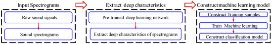
Figure 2.
Basic idea of automatic recognition method-based spectrograms: input spectrograms, extract deep characteristics, and construct machine learning model.
First, spectrograms are chosen as the input indicator for crack type recognition. In traditional sound recognition, time-domain parameters such as the Mel-frequency cepstral coefficient (MFCC) and short-term energy are used as indicators. Compared with the traditional indicators, the spectrogram, which can visualize the time-frequency distribution of the sound signal, is more comprehensive [19,20]. In addition, sound recognition with spectrogram can decrease the adverse influence of many factors, for example, the artificially chosen step lengths of the sound signals. Consequently, the spectrogram is more powerful than other indicators during sound recognition.
Second, the characteristics of the spectrogram are extracted using the pre-trained deep learning method. Deep learning methods perform excellently in the field of image recognition. In traditional deep learning, complex network structures are used to find reasonable classification explanations from a large amount of image data without specifying the specific characteristics of the image. In other words, the best parameters of deep learning models are identified based on a tremendous amount of training samples. If a small training sample is considered, the generalization ability of the models will be weakened, and overfitting problems will be encountered. However, in the field of rock engineering, only a limited number of signals can be obtained, which results in small sample problems. Using small samples to train deep learning networks is not possible. Compared with shallow machine learning, the greatest advantage of deep learning is the ability to transfer features. For deep learning methods, pre-trained deep learning network models established by a large data set can be used to easily extract features for other datasets, which is called feature-based migration learning. The pre-trained deep learning networks can be conveniently applied to other classification problems. Bousetouane and Morris [21] pointed out that the convolutional neural network model pre-trained on the ImageNet dataset can be used as a good feature extractor for unknown image sets. Many researchers [22,23,24,25] have suggested that using the deep characteristics of images extracted by pre-trained deep learning models results in a better classification performance than that using most artificially described features such as textures and edges. The pre-trained deep learning model can be used as an automatic feature extractor to not only obtain rich features describing the image but also to reduce the burden of manual extraction and facilitate image classification.
Third, Gaussian process classification (GPC), a classical machine learning method, is used to establish the implicit mapping relations between the input (the deep characteristic of the tensile and shear spectrograms from the pre-trained deep learning networks) and the output (tensile and shear crack types). Unlike deep learning methods requiring the classification of large data samples, machine learning has a strict statistical theory. Even with small sample problems, GPC exhibits excellent robustness and generalization ability. Thus, based on the output characteristic of the spectrograms, GPC is employed for determining the crack types of the spectrograms.
Through the above strategy, the proposed method combines the deep learning method and shallow machine learning method to complement each other. On the one hand, the method utilizes deep learning to automatically extract the deep characteristics of images, reducing the burden of manually extracting features. On the other hand, GPC is used to establish implicit mapping relations between the sound signal characteristics and crack types on a small spectrogram training set, which avoids the overfitting problem during iterative training in deep learning methods. In the end, the classification model is applied to an actual analysis to verify its accuracy.
2.2. Sound Signals of Tensile and Shear Cracks Collected during Rock Tests
2.2.1. Rock Tests
Tensile cracks dominate the rock failure during Brazilian splitting testing, while, in the direct shear test, shear cracks are the dominant force causing the rock failure. By conducting the corresponding tests, the sound signals of tensile and shear cracks are first collected. The corresponding rock specimens, testing machines, loading schemes, and obtained sound signals are presented as follows.
The rock material used is coarse red granite obtained from Wuhan city, Hubei Province, China. Several of the physical and mechanical parameters of the rock material are listed in Table 1. The rock specimens used are shown in Figure 3. A disc specimen (Figure 3a) with a diameter of 100 mm and thickness of 40 mm is used to conduct the Brazilian splitting tests. A cubic specimen (Figure 3b) with a side length of 100 mm is used to conduct a direct shear test.

Table 1.
Physical and mechanical parameters of the rock specimens.
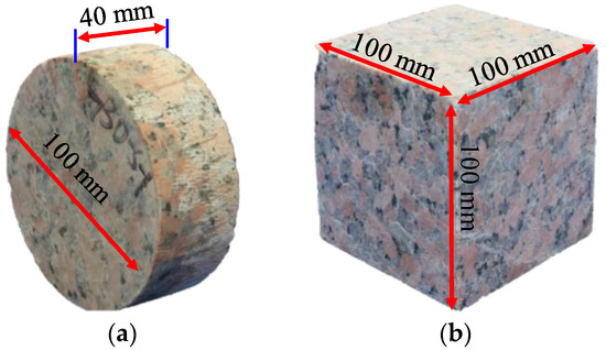
Figure 3.
Rock test specimens of (a) disc granite specimen for the Brazilian splitting test to collect the sound of tensile cracks and (b) cube granite specimen for the direct shear test to collect the sound of shear cracks.
To conduct the Brazilian splitting and direct shear tests, a true triaxial rockburst machine (Figure 4), which is highly rigid, with a stiffness of 9000 kN/mm in the vertical direction and 5000 kN/mm in the horizontal direction, is used. This machine can load/unload along three mutually orthogonal directions independently, and it allows the application of a vertical force of 5000 kN and a lateral force of 3500 kN via a servo control system.
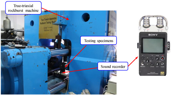
Figure 4.
Experimental setup: True-triaxial rockburst machine testing system and sound recorder.
As shown in Figure 4, the PCM-D100 voice recorder produced by Sony Corporation is used to monitor the sound signals. The sample rate of the recorder is 192 kHz. During the testing process, the recorder is located approximately 20 cm from the tested specimen. A quiet environment is needed to obtain a high-quality sound signal.
The loading device for the Brazilian splitting test is presented in Figure 5a. The corresponding loading path is described as follows. A load of 5 kN is first applied at a rate of 50 N/s on the tested specimen along the vertical direction; then the load is increased at a rate of 500 N/s until the tested specimen fails. The loading device for the direct shear test is presented in Figure 5b. The corresponding loading path is described as follows. A vertical load of 10 kN and a horizontal load of 5 kN are applied to the tested specimen at a rate of 500 N/s; then the vertical load is kept constant, and the horizontal load is increased at a rate of 500 N/s until the specimen fails. In addition, the specimen number and testing scheme used in each test are shown in Table 2.
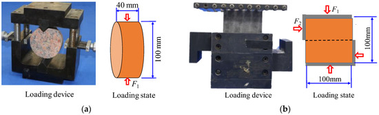
Figure 5.
Loading device and stress state of the tested specimen in (a) Brazilian splitting test and (b) direct shear test.
Table 2.
Loading scheme.
2.2.2. Sound Signals of Tensile and Shear Cracks
The waveforms of the obtained sound signals are presented in Figure 6. It can be seen that the sound signal of the tensile crack from the Brazilian splitting test is different from that of the shear crack from the direct shear test.
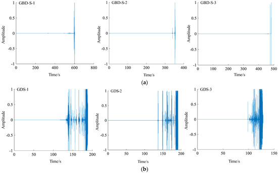
Figure 6.
Waveform of the tested specimen from (a) the Brazilian splitting test and (b) the direct shear test.
Figure 6a shows the sound signal obtained from the Brazilian splitting test. In the early stage of the test, the rock specimens are in a calm state, and there are no cracking sounds. In the late stage of the test, a small number of cracking sounds appeared gradually. The amplitude of these signals is low, indicating the small-scale failure in the specimen. At the end of the test, the sound signal with the maximum amplitude occurs, and the final macro failure occurs quickly. The dull “bang” sound can be heard by the human ear.
Figure 6b presents the sound signal from the direct shear test. In the early stage of the test, there are still no cracking sounds. After loading for a while, although the cracks of rock specimens are invisible due to the obstruction of the loading device, the successive ringing of a “ka” sound can be detected by the human ear, indicating the successive formation of small cracks. The waveform of sound signals at this stage is dense. In the late stage of the test, the rock specimens produce a continuous sound of frictional fracture between the rock grains. The cracking sounds gradually increase, and it changes from crisp to low. At the end of the test, the final failure of the rock specimen occurs with the dull “bang” sound, the corresponding waveform of sound signals is denser, and the amplitude of the sound signal is higher.
It should be pointed out that to eliminate the influence of noise, the obtained sound signals should be first filtered before being processed.
2.2.3. Extracting Spectrograms of the Tensile Cracks and Shear Cracks
Taking the tested specimens GBD-S-2 and GDS-2 as examples, the extracting spectrograms are described in detail as follows.
First, because the obtained sound signals are non-stationarity, “framing” should be performed to ensure that the sound signal is “smooth” within this frame length. Changes between two adjacent frames will affect the subsequent feature extraction of the sound signals, including tone color, tone, and other parameters of the sound signals. Therefore, the interval between the two frames is set, which is also called the frame shift. The overlap between the two frames can be calculated by overlap = frame length—frame shift. The frame of the signal is shown in Figure 7, and the frame parameters are determined as follows: the frame length is 10 ms, and the frame shift is 5 ms.
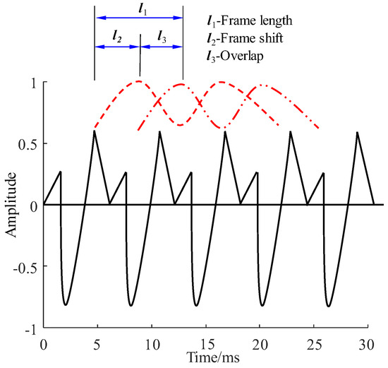
Figure 7.
Framing the sound signal with the given frame length, frame shift, and overlap.
Second, windowing should be performed. Fourier transform is generally employed to obtain the frequency domain representation of the signal. In our study, the short-time Fourier transform (STFT) was used to draw the sound spectrograms. When the signal is truncated, there will be a “leakage” of spectrum energy during the Fourier transform. To reduce the impact caused by the discontinuities and reduce the leakage of the spectrum energy, window functions should be used to intercept the signals. We choose the Hamming window to avoid spectrum energy leakage. The calculation principle of the Hamming window is as follows [26]:
As an improved cosine window, the side lobe of the Hamming window is small and the side lobe attenuation speed of the Hamming window is slow, which can more effectively approach the spectrum of the original speech and avoid spectrum leakage.
Third, the duration of the time-domain sound signal corresponding to a crack, a single sound signal, was determined. The general duration of a single sound signal used in current sound recognition is 10–50 ms. Considering the sampling frequency of the sound recording instrument used in this work, the duration used was 20 ms. With this duration, the sound signals were intercepted as shown in Figure 8.
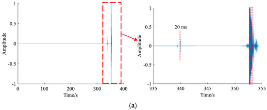
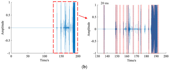
Figure 8.
Selecting the objective sound signals with a time interval of 20 ms obtained from (a) Brazilian splitting test on the specimen GBD-S-2 and (b) direct shear test on the specimen GDS-2.
Then the short-time Fourier transform (STFT) to sound signal was implemented to obtain the spectrograms, and the calculation formula of STFT is as follows:
In this formula, Xn is the speech signal sequence, w(m) is the window function, and w is the frequency. With the transformation of the sequence variable n, the Fourier transform result of the entire signal at different frame positions can be achieved.
The typical spectrograms of the tensile and shear sound signals are presented in Figure 9. In each spectrogram, the abscissa indicates time, and the ordinate indicates the frequency. The color indicates the amplitude: as the color changes from blue to red, the amplitude increases. Therefore, the spectrograms can express the dynamic time-frequency amplitude of the sound signal. Obviously, from the perspective of texture and color of spectrograms, there are some differences between the tensile spectrograms and shear spectrograms. In addition, the characteristics of the spectrograms are described in detail in Table 3.
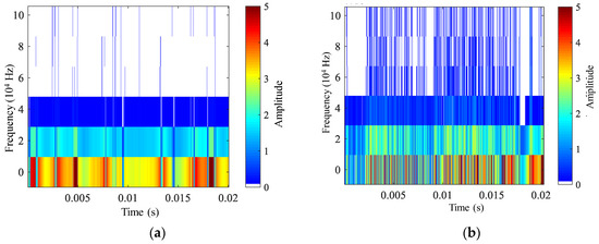
Figure 9.
Sound spectrograms of typical (a) tensile and (b) shear cracks.
Table 3.
Characteristics of tensile and shear spectrograms.
The spectrogram of the tensile crack shows an aggregate “bar” form in the short interval. The main frequency ranged from 0 to 30 kHz. The duration of high energy was wide, and the high energy ranged from 3 to 5 with a duration of approximately 0 to 0.02 s. The maximum energy was 5, occurring at 0.0048 s and 0.018 s. These characteristics indicate that the formation of tensile cracks corresponds to a stable energy release process.
The spectrogram of the shear crack shows a jumbled “jungle” form in the short interval. The main frequency ranges from 0 to 100 kHz. The duration of the high energy was narrow and dispersed, and the high energy ranged from 4 to 5 with a duration of approximately 0.005 to 0.02 s. The maximum energy was 5, occurring at 0.016 s and 0.02 s. These characteristics indicate that the formation of shear crack corresponds to a more successive and dispersed energy release process.
2.3. Feature Extraction Using a Pre-Trained Deep Neural Network ResNet-18
2.3.1. ResNet-18 Network
In traditional plain convolutional neural networks(CNN), with the increase in the network net, a deeper characterization of the image can be obtained by the convolutional kernel. However, gradient diffusion will be encountered, which results in an increase in the error of the information transfer between networks and causes a further decrease in the accuracy of the output. To address this problem, He et al. [27] proposed the deep residual network model. The basic idea of residual mapping can be described as shown in Figure 10. Assume that x is the input, H(x) is the expected output and is expressed by H(x) = F(x) + x, and F(x) = H(x) − x is the residual mapping. This mapping relationship is different from that of H(x) = x. During the training of the model, the optimal object is F(x) infinitely approaching 0. With this development, the origin information of the sample can be kept during the iterative training in the deep learning network, which avoids gradient diffusion.
where σ is the activation function ReLU, and W1 and W2 are the calculations of the first and second weight layers, respectively. By establishing a shortcut connection, the mapping relationship can be expressed by Equation (4). When the dimension of the shortcut connecting x is different from that of F(x), a convolutional process Ws can be added to adjust the corresponding dimension, as shown in Equation (5).
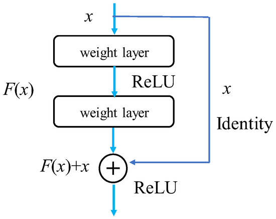
Figure 10.
Residual learning of F(x) = H(x) − x [27].
In the ResNet network, the residual can be either a two-layer type or a three-layer type of residual, as shown in Figure 11:
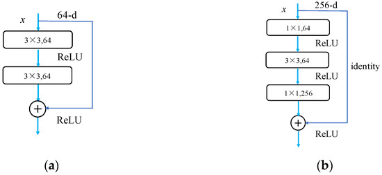
Figure 11.
Residual blocks in the ResNet network [27]: (a) Two-layer residual block; (b) Three-layer residual block.
The deep learning ResNet network can resolve gradient diffusion when the number of layers increases. This does not mean that more layers correspond to a better output. When the number of layers is higher than 1000, the addition of a layer will not increase the accuracy of the output but will significantly increase the calculation time. To balance the accuracy of the classification and calculation time, pre-trained ResNet-18 is used to extract the characteristics of the spectrograms. The ResNet-18 framework is shown in Figure 12. In this study, the used network was sourced from Matlab.
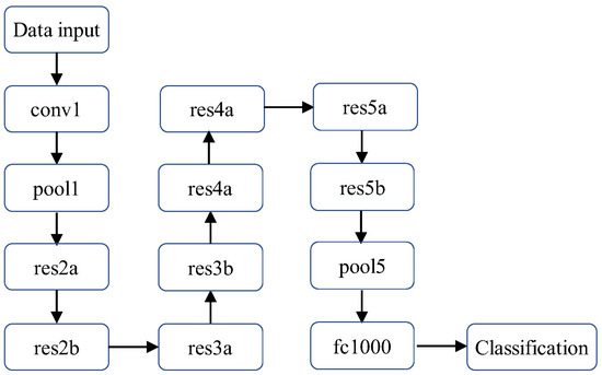
Figure 12.
Structure of the deep residual network ResNet-18 [27].
2.3.2. Feature Extraction from the Spectrograms
As shown in Figure 12, there are several convolutional layers (conv1, pool1, res2a, res2b, and so on) in ResNet-18. To better extract the characteristics of the spectrograms, the most suitable convolutional layer should consider the following two issues.
The first is to consider whether the convolution can extract the characteristics of the spectrograms well. Except for the classification layer, each layer in ResNet-18 can be used. The spectrograms shown in Figure 9 are input into ResNet-18; the visualization of the spectrogram characteristics from the conv1 layer, the res2a layer, and the pool5 layer are shown in Figure 13. It can be seen that, for the ResNet-18, the characteristics of the figures extracted by the shallow convolution layers are mainly described by the texture and color. When a deeper network layer is used, a deeper characteristic of an image will be obtained and the corresponding characteristic is more abstract. However, according to previous studies, more abstract results can better present the characteristics of the figure [28,29,30]. Meanwhile, the use of residual blocks in ResNet-18 can effectively resolve the gradient diffusion. Consequently, in our study, a deeper layer after res5b is used to capture the characteristics of the tensile and shear spectrograms.
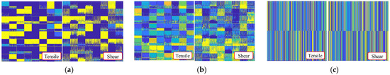
Figure 13.
Visualization of the spectrogram characteristics of the typical tensile and shear cracks extracted by (a) the conv1 layer, (b) the res2a layer, and (c) the pool5 layer.
The second is that, to ensure the efficiency of calculation, the dimension of the characteristics should not be too high. First, the RGB value of a figure is input into ResNet-18. A characteristic matrix with dimensions of 224 × 224 × 3 is obtained. Then, after pooling by the maximum pooling layer pool1, the dimensions of the characteristic matrix are 56 × 56 × 64. The residual block is the connected convolutional layers. The residual block res2a is composed of two convolutional layers with dimensions of 3 × 3 × 64, and the residual block res2b is composed of three convolutional layers with dimensions of 1 × 1 × 64, 3 × 3 × 64 and 1 × 1 × 256. After res5b, the dimensions of the output characteristic are 7 × 7 × 512. After the average pooling calculation of the pooling layer pool5, the output dimensions are 1 × 1 × 512; after the fully connected layer “fc1000”, the output dimensions are 1 × 1 × 1000. During this process, the dimensions of the output characteristic will increase at the residual blocks and decrease after the pool5 layer.
Consequently, the characteristic of a spectrogram extracted by pool5 is the most suitable. First, pool5 is a deep layer (only fc1000 and the classification layer are deeper), and the output characteristic will be complicated enough to describe the objective figure. The dimension of the characteristic matrix is 512, which is smaller than that of other layers.
The visualization of the characteristics of the tensile and shear spectrograms extracted by the pool5 layer is presented in Figure 13c.
2.4. Identification Model for Tensile and Shear Crack Using GPC
Based on the deep characteristics of spectrograms extracted by using the pooling layer of pre-trained ResNet-18, GPC is used to establish an implicit mapping relation between the sound characteristics (input) and crack types (output).
2.4.1. Basic Principle of GPC
The Gaussian process (GP) is a machine learning technology based on Bayesian statistical learning theory, and it exhibits excellent performance in solving nonlinear, small-sample, and high-dimensional problems [31]. In addition, it has the advantage of automatically obtaining hyper-parameters and providing a probability interpretation of the output. It is therefore commonly applied in many fields, such as structure reliability analysis, structure optimization, and signal processing [32,33,34].
There is a training set D = {(xi, yi)|I = 1, 2, 3, 4, …, N}. The set of input variables is X = [x1, x2,x3,x4….xN]T. The function value of the input variables set is Y = [y1, y2, y3, y4….yN]T. When a binary classification problem is calculated, the range of the y value is assumed to be yi ∈ {−1, 1}. The set of prediction samples is f = [f1, …, fn]T; fi = f(xi).
The basic assumption of Gaussian process classification (GPC) is that the prediction function f conforms to the prior distribution of the Gaussian process, and the response function Φ(x) is used to “compress” the function range to the interval [0, 1], making the classification probabilistic. The probability of the first-class classification is p(y = +1), then
Similarly, in binary classification, the sum of the probabilities of the entire probability space is 1, so the probability of p(y = −1) is .
According to Bayesian theory, the posterior distribution of the latent function can be obtained as
where and , assuming that the prior distribution of the latent function obeys the standard normal distribution function N (0, K), where K is an n × n order covariance function matrix. The covariance function commonly used in general Gaussian processes is covNNone:
Thus, the posterior distribution of the objective function is given by
Based on the learning process of GPC, the prediction is divided into two steps. First, the probability of the posterior function value f∗ corresponding to the test point x∗ is
According to the above formula, the predicted probability of the posterior distribution of p (y = +1) can be further calculated:
In Equation (11), Φ(f∗) represents the classification probability corresponding to the test point function value f∗. The classification prediction probability distribution of f∗ can be calculated by Equation (10).
Second, classification types are divided according to probability. In the Gaussian process classification (GPC), the minimum misclassification rate is regarded as the threshold. For binary classification problems, p (y∗ = +1|X, y, x∗) = 0.5 is usually used as the classification limit. When p is greater than 0.5, y∗ = +1 belongs to the first category, and when p is less than 0.5, y∗ = −1 belongs to the second category.
2.4.2. Implementation Steps
There are four main steps, including data collection, training samples construction, recognition model establishment, and prediction samples recognition, involved in the application of the proposed method, as shown in Figure 14 and described in the following sections.
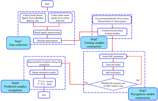
Figure 14.
Flow chart of the proposed method with four steps: data collection, training sample construction, prediction sample recognition, and recognition model construction.
Step 1: Collect tensile and shear sound signals. The sound signals of tensile cracks are collected from Brazilian splitting tests, and the sound signals of shear cracks are collected from direct shear tests. A sound sample set including both sound signals is established.
Step 2: Pre-process the sound signals by denoising, framing, and adding windows.
Step 3: Generate spectrograms. The short-time Fourier transform (STFT) is used to draw the sound spectrograms.
Step 4: Extract characteristics of the spectrograms using pre-trained ResNet-18. The pool5 layer of ResNet-18 is used to extract the deep characteristics of spectrograms. All spectrograms in the sample set are extracted deep characteristics to construct training samples to train the GPC model.
Step 5: Establish the GPC model. Before iterative training, some initial parameters of the GPC model that need to be determined include the initial hyper-parameter range, kernel function type, and adaptive parameter optimization times. These necessary parameters are finally determined after iterative training.
Step 6: Verify the GPC model. During the training process, the trained GPC model is self-validated. If the accuracy of the verification results meets the requirements, the determination method is accurate, and the next step is continued. Otherwise, return to step 5; the distribution of training samples or the initial parameters of the GPC model must be adjusted again.
Step 7: Input the prediction sample. All the predicted sound signals are processed according to steps 2–4, and the corresponding deep characteristics of the spectrograms are extracted. The extracted characteristics are used as inputs to the trained GPC model in order to obtain the final classification probability. According to the output results, the crack type can be predicted. The meaning of the output probability p* of the GPC model is as follows: When p* > 0.5, the sound signal is determined to be a tensile signal. The closer the p* value is to +1, the greater the probability that the sound signal is a tensile crack. When the probability value is p* < 0.5, the sound signal is predicted to be a shear signal. The closer the p* value is to −1, the greater the probability that the sound signal is a shear crack.
A MATLAB-based program was developed according to these steps.
2.4.3. Verify the GPC
To verify the proposed method, the cross-validation method is used to test the robustness of the proposed method. The cross-validation method is described as follows: the data set is randomly divided into k equal parts; k − 1 parts are used as training samples each time, and the remaining part is used as a testing sample. The test is repeated for k times, and the average accuracy of all repetitions is taken as a final evaluation of the model performance.
In the verification of this method, k is 5, and all training samples (a total of 40 spectrograms, 23 of tensile cracking and 17 of shear cracking) are randomly divided into 5 parts, each of which includes 8 spectrograms, and the test is verified 5 times. The average accuracy rate of the 5 times test is taken as the evaluation index of the method. The GPC initial hyper-parameter is [−2; 2]. The number of repetitions used to optimize the adaptive hyper-parameter is 30. The GPC kernel function is covNNone.
Table 4 shows that the average accuracy of this method reaches 90%. Under the condition of a small sample, the recognition method in this paper has an extremely strong generalization ability and a high recognition accuracy.
Table 4.
Results of the cross-validation of the proposed method.
3. Results and Discussion
3.1. Identifying the Development of Tensile and Shear Cracks under Biaxial Compression Test
3.1.1. Biaxial Compression Test on a Granite Specimen
Crack development during rock failure under biaxial compressive conditions can be effectively characterized by experimental studies. In the early stage of rock failure, splitting (tensile) cracks first occur on both sides of the rock specimens. At the late stage, especially just before rock failure, shear cracks occur in the middle of the tested specimen. Considering this crack development, the method proposed in our study can be verified.
First, a biaxial test on granite is conducted. The testing equipment used is described in Section 3.1. The cuboid granite specimen has dimensions of 100 mm (length) × 100 mm (width) × 200 mm (height). The loading device is shown in Figure 15. The testing process can be described as follows. First, pre-stresses: a vertical stress σz of 0.5 MPa and a horizontal stress σx of 0.25 MPa are applied to the tested specimen. Then σx is increased to 1 MPa at a rate of 0.05 MPa/s and held constant. σz is increased continually at a rate of 0.5 MPa/s until the specimen fails. The failed specimen is shown in Figure 16.
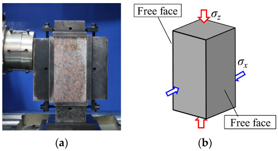
Figure 15.
Biaxial compression test: (a) rock specimen and loading device, (b) stress state of the specimen.
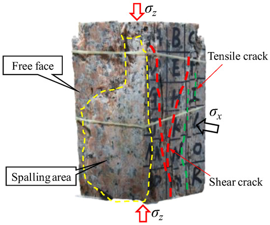
Figure 16.
Failed specimen after the biaxial test.
According to the change characteristics of the stress–strain curve, the pre-peak deformation can be divided into four stages, as shown in Figure 17: A: initial compaction stage, B: linear elastic stage, C: elastic–plastic transition stage, and D: plastic stage. The raw sound signal is also divided according to the corresponding four stages, as shown in Figure 18. Since the rock specimens have failed in the post-peak period, the recording of sound signals is stopped in that stage after 119.4 s. From 0 to 56.743 s, there are no sound signals. From 56.743 to 119.4 s, the sounds occur sporadically throughout the recording time.
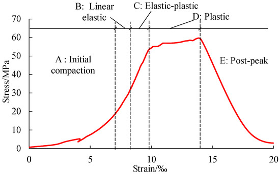
Figure 17.
Stress–strain curve of tested granite specimen from the biaxial compression test.
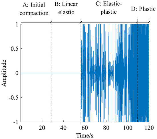
Figure 18.
Waveform of the sound signal obtained from the biaxial compression test.
3.1.2. Tensile and Shear Cracks Development under Biaxial Compression Test
The tensile and shear crack development during rock failure under biaxial conditions was determined as follows. Occurring sporadically throughout the recording time during the biaxial test, the cracking sound signals are divided into sections with a time interval of 20 ms. After obtaining all the intercepted sound signals, the spectrograms are extracted to construct the prediction sample. Then, the deep characteristics of the predicted spectrograms are extracted from the pool5 layer of the pre-trained ResNet-18; the corresponding operational process is described in Section 3.2. The characteristics are used as input to a trained GPC to obtain the final recognition results of the crack types. The related parameters of trained GPC during identification are set as follows. The training sample comprises 48 spectrograms. The GPC initial hyper-parameter is [−2; 2]. The number of repetitions used to optimize the adaptive hyper-parameter is 30. The GPC kernel function is covNNone.
The variation of tensile and shear sound signals obtained using the proposed method is shown in Figure 19. In the figure, the abscissa indicates the time when the sound signal of the crack occurs, and the ordinate indicates the predicted probability of GPC. When the predicted probability of GPC is greater than or equal to 0.5, a tensile crack is predicted, and when it is less than 0.5, a shear crack is predicted. The proportions of tensile and shear sound signals in different deformation stages are shown in Table 5. During the initial compaction stage (0–28.8 s) and the elastic stage (28.8–56.743 s), there is no crack sound appearance. In the elastic–plastic stage (56.743–109.44 s), the cracking activity inside the rock increases, and the number of sound signals increases. The first cracking sounds occur at 56.753 s. During this stage, the sound signals are mainly tensile type, and only a small amount of shear sound signals occur; tensile sound signals account for 85%. During the plastic stage (109.44–119.4 s), the number of shear sound signals continually increases, the proportion of the shear sound signals accounts for more than 75%.
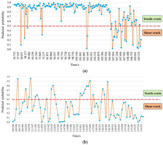
Figure 19.
Variation in the tensile and shear sound signals in different stages using the proposed method under biaxial test: (a) elastic–plastic stage; (b) plastic stage.
Table 5.
Proportions of tensile and shear sound signals in different stages under biaxial test.
The tensile and shear crack development during rock failure under biaxial conditions is shown in Figure 20. The rock specimen undergoes a typical process from tensile crack development on both sides to internal shear cracks, which is consistent with previous research [35]. Consequently, it can be seen that the proposed method is feasible.
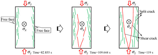
Figure 20.
Tensile and shear crack development process under biaxial compression test.
3.2. Identifying the Development of Tensile and Shear Cracks during Rockburst
Rockburst is an engineering geological disaster that occurs during underground excavation at depth [36,37]. Accompanied by rock block ejection, rockburst poses a great threat to workers and construction equipment [38]. Rockburst is a complicated dynamic rock failure. Identifying the corresponding development of tensile and shear cracks is important for revealing the mechanism of rockburst. In the following section, the proposed method is used to identify the tensile and shear cracks during rockburst produced by using a laboratory testing machine.
3.2.1. Rockburst Test on a Granite Specimen
In our study, the true-triaxial rockburst testing machine developed at Guangxi University, China, is used to simulate the rockburst process. As shown in Figure 21, a loading path, “one free face, five stressed faces” is used, and the tested cuboid specimen has dimensions of 100 mm (width) × 100 mm (length) × 200 mm (height) [39]. The loading plan can be described as follows: σx and σy are increased to 30 MPa and 5 MPa; simultaneously, σz is increased at a rate of 0.3 MPa/s until the rock specimen fails.
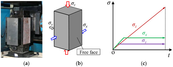
Figure 21.
Rockburst test (a) size and shape of the rock specimen and loading device, (b) stress state of the specimen, (c) loading path.
During the testing process, the voice recorder for collecting the sound signal is located approximately 20 cm from the tested specimens. The failure form of the tested specimen is shown in Figure 22. The tested specimen shows a binary failure characteristic, where more serious failure occurs at the free faces. A rockburst pit can be observed, and the surface of the rockburst pit is covered by rock fragments and powders. In addition, near the free face, a vertical tensile (splitting) crack can be observed. Away from the free face, several oblique cracks develop, and a lot of white powders are observed on the crack face, indicating a shear failure characteristic. It can be concluded that rockburst is characterized by the external tensile crack on the free face and the internal shear crack away from the free face. Consequently, an investigation on the development of tensile and shear cracks can provide beneficial information for the revelation of rockburst mechanisms.
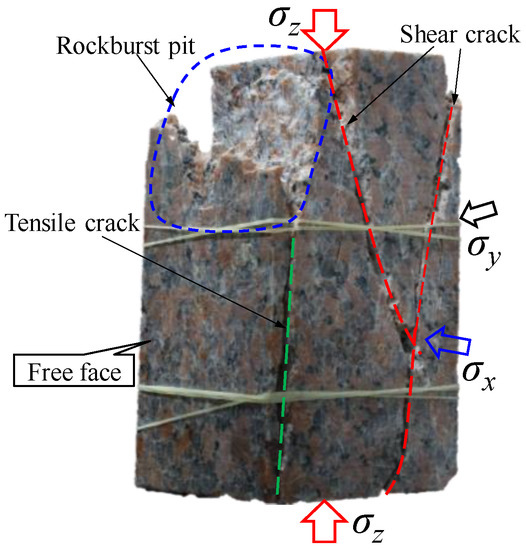
Figure 22.
Failed specimen after the rockburst test.
According to the characteristics of the stress–strain curve, the pre-peak deformation can be divided into four stages, as shown in Figure 23: A: initial compaction stage, B: linear elastic stage, C: elastic–plastic transition stage, and D: plastic stage. From 0 to 519.621 s, there are no sound signals. From 519.621 to 742.447 s, the sounds occur sporadically. The characteristics of the sound signal in the different stages are described in detail as follows.
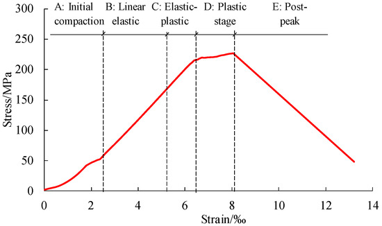
Figure 23.
Stress-strain curve from the biaxial compression test.
In the crack compaction stage (0–167.76 s), pre-existing cracks close, which is an extremely slight rock deformation behavior; in the elastic deformation stage (167.76–519.621 s), there are no crack sounds. In elastic–plastic deformation (519.621–700.92 s), a large number of sound signals with high amplitude occur, which can be detected by not only sensors but also the human ear. The waveform is dense because many cracks continually develop and propagate, and local failure caused by unrecoverable plastic deformation occurs. Then, the plastic deformation stage (700.92–742.447 s) is encountered. In this stage, more high-amplitude sound signals occur, intensive rockburst occurs, and a large number of rock blocks are ejected from the free face.
3.2.2. Tensile and Shear Cracks Process during Rockburst
The identification of tensile and shear cracks during rockburst is presented as follows. All the predicted sound signals are processed according to Section 3.
The related parameters of trained GPC during identification are set as follows. The training sample comprises 48 spectrograms. The GPC initial hyper-parameter is [−2; 2]. The number of repetitions used to optimize the adaptive hyper-parameter is 30. The GPC kernel function is covNNone.
The variation in the tensile and shear sound signals obtained using the proposed method is shown in Figure 24. The abscissa indicates the time when the sound signal of the crack occurs, and the ordinate indicates the predicted probability of GPC. When the predicted probability of GPC is greater than or equal to 0.5, a tensile crack is predicted, and when it is less than 0.5, a shear crack is predicted. The proportions of tensile and shear crack sound signals in different deformation stages are shown in Table 6. It can be seen that sound signals caused by tensile cracks occur in the early stage of rockburst, and shear cracks occur in the late stage. In the elastic–plastic stage (519.621–700.92 s), the tensile sound signals account for 92%. The proportion of the shear sound signal rises to approximately 8%. During the plastic stage (700.92–742.447 s), the number of shear sound signals continually increases, and the proportion of the shear sound signals accounts for more than 80%.
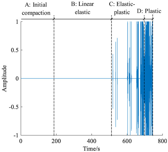
Figure 24.
Waveform from the rockburst test.
Table 6.
Proportions of tensile and shear sound signals in different stages under rockburst.
According to the recognition results of the sound signals using the proposed method, the tensile and shear crack development can be obtained as follows. In the compaction and linear elastic stage, only a few micro cracks initiate, and no macro cracks can be observed. In the elastic–plastic deformation, these cracks will propagate to cause the formation of macro cracks. The sliding along the macro cracks will cause the development of shear cracks, leading to unrecoverable plastic deformation. With more cracks propagating, more shear cracks occur, which causes the formation of the predominant cracks and the final failure. In this process, if the released energy cannot be dissipated by the shear cracks, the residual energy will be translated into the kinetic energy of ejected fragments, leading to the formation of rockburst.
Based on the results of the tensile–shear crack evolution and the failure process of the rock specimen during rockburst, the incubation mechanism of rockburst can be better summarized, as shown in Figure 25. In the rockburst test, the failure of the specimen gradually progresses with the loading of the stress. Under the applied stress σx, σy, and σz, the rock specimen gradually becomes dense. At this time, due to the nonuniform grain size, the three-dimensional stresses remain low, and a small number of cracking events occur in the rock. As σz continues to increase, the rock specimen is fractured by compression, and a large number of tensile cracks form parallel to the z direction, but, at this time, σz is still low. Due to the Poisson effect, under the force in the x and y directions, the large-scale destruction of the rock specimen on the free surface is suppressed. As σz continues to increase, the slab-compression-induced splitting phenomenon continues to occur, and tensile cracks also form and expand. In the vicinity of the free surface, the σy value is close to 0, and the inhibition effect is low. Significant swelling appears near the free surface element, but, as the rock specimen element is further away from the free surface, σy also gradually increases, so the inhibitory effect becomes increasingly obvious. Under the applied forces, the relative friction and sliding between the cracks promote the increase in shear cracks, which creates conditions for the potential shear zone. As σz gradually increases until the rock specimen loses its bearing capacity, a large amount of strain energy is stored inside the rock specimen from loading to this stage. According to existing studies [39], most of the strain energy stored in a rock specimen that passes through an internal shear dislocation dissipates. At this time, many shear cracks, which are the main cause of the energy dissipation, form, and a macroscopic oblique shear zone that penetrates the rock specimen is formed. In addition, the remaining strain energy will be consumed by block ejection from the free surface. Therefore, with the loud noise of the macroscale destruction of the rock specimen, a large number of blocks from the free surface are ejected outward, and rockburst occurs. According to our recognition results during crack type development, tensile cracks dramatically decrease and shear cracks rapidly increase, which can be taken as an indicator of rockburst.
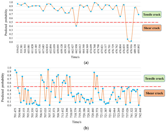
Figure 25.
Variation in the tensile and shear sound signals atg different stages using the proposed method under rockburst: (a) elastic–plastic stage; (b) plastic stage.
In summary, based on the identification results using the proposed method, there is a transition from the early stage of tensile crack initiation, propagation, and coalescence to the late stage of shear crack occurrence during rockburst process (Figure 26), which is consistent with crack development during rockburst in previous studies [39,40], which again indicates that the proposed method is feasible.
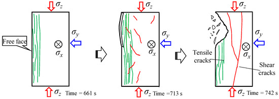
Figure 26.
Tensile and shear crack development process during the rockburst test.
4. Conclusions
Rock failure is closely related to crack development. The identification of crack type (tensile or shear crack) can provide beneficial information to understand crack development and further reveal the rock failure mechanism. In our study, using sound signals, a method for automatically identifying the type of crack that develops in rock is proposed. This method takes advantage of the deep learning method and the shallow machine learning method. In this proposed method, sound signals corresponding to tensile cracks and shear cracks are first collected from Brazilian splitting tests and direct shear tests, respectively, to establish the training sample dataset. Abstract features that distinguish the corresponding spectrograms of sound signals are extracted by using the pooling layer of a pre-trained ResNet-18. GPC, a supervised learning method adaptable to the analysis of small samples, is trained to establish the crack type identification model.
Application in biaxial tests indicates that the proposed method is feasible. In addition, the proposed method is used to investigate crack development during rockburst. The study results indicate that the early stage of rockburst is dominated by tensile cracks, while shear cracks dominate the late stage of rockburst. The obtained result is consistent with those of previous studies, which further indicates the feasibility of the proposed method.
In this paper, the proposed method has the advantages of low cost and easy implementation. Compared with the traditional identification method using AE signals, the proposed method overcomes limitations of objective factors such as the number of sensors or unstable contact between the acoustic emission sensor and the rock mass. In addition, the proposed method based on sound signals provides a new way to deepen the understanding of the mechanism of rock failure and can help further realize the early warning of rock failure. However, the method in our study is proposed based on lab testing, and many influencing factors, such as the sample shape and also position of the microphone, have not been considered in the preliminary stage of this study. The application of the proposed method to on-site practice will be conducted in our future work. In addition, it should be pointed out that the proposed method is a supplement instead of a replacement of the pre-existing methods to crack type identification.
Author Contributions
Conceptualization, H.J.; methodology, G.S.; validation, H.J.; investigation, H.J. and J.J.; data curation, J.J.; writing—original draft preparation, H.J.; writing—review and editing, H.J. and J.J.; funding acquisition, G.S. All authors have read and agreed to the published version of the manuscript.
Funding
This research was funded by the National Natural Science Foundation of China (Grant No. 52169021, 51869003) and the High-Level Innovation Team and Outstanding Scholar Program of Universities in Guangxi province. (Grant No. 202006).
Institutional Review Board Statement
Not applicable.
Informed Consent Statement
Not applicable.
Data Availability Statement
Not applicable.
Conflicts of Interest
The authors declare no conflict of interest.
References
- Jiang, J.; Su, G.; Yan, Z.; Hu, X. Rock crack type identification by Gaussian process learning on acoustic emission. Appl. Acoust. 2022, 19, 108926. [Google Scholar] [CrossRef]
- Ohno, K.; Ohtsu, M. Crack classification in concrete based on acoustic emission. Constr. Build. Mater. 2010, 24, 2339–2346. [Google Scholar] [CrossRef]
- Aggelis, D.G. Classification of cracking mode in concrete by acoustic emission parameters. Mech. Res. Commun. 2011, 38, 153–157. [Google Scholar] [CrossRef]
- Aggelis, D.G.; Mpalaskas, A.C.; Matikas, T.E. Acoustic signature of different fracture modes in marble and cementitious materials under flexural load. Mech. Res. Commun. 2013, 47, 39–43. [Google Scholar] [CrossRef]
- Liu, J.; Li, Y.; Xu, X.; Xu, S.; Jing, C. Cracking mechanisms in granite rocks subjected to uniaxial compression by moment tensor analysis of acoustic emission. Theor. Appl. Fract. Mech. 2015, 75, 151–159. [Google Scholar]
- Zhou, H.; Wang, Z.; Ren, W.; Liu, Z.; Liu, J. Acoustic emission based mechanical behaviors of Beishan granite under conventional triaxial compression and hydro-mechanical coupling tests. Int. J. Rock Mech. Min. Sci. 2019, 123, 104125. [Google Scholar] [CrossRef]
- Li, D.; Wang, E.; Kong, X.; Ali, M.; Wang, D. Mechanical behaviors and acoustic emission fractal characteristics of coal specimens with a pre-existing flaw of various inclinations under uniaxial compression. Int. J. Rock Mech. Min. Sci. 2019, 116, 38–51. [Google Scholar] [CrossRef]
- Hu, X.; Su, G.; Chen, G.; Mei, S.; Feng, X.; Mei, G.; Huang, X. Experiment on Rockburst Process of Borehole and Its Acoustic Emission Characteristics. Rock Mech. Rock Eng. 2019, 52, 783–802. [Google Scholar] [CrossRef]
- Meng, F.; Zhou, H.; Wang, Z.; Zhang, L.; Kong, L.; Li, S.; Zhang, C. Influences of Shear History and Infilling on the Mechanical Characteristics and Acoustic Emissions of Joints. Rock Mech. Rock Eng. 2017, 50, 2039–2057. [Google Scholar] [CrossRef]
- Chen, B.; Feng, X.; Li, Q.; Luo, R.; Li, S. Rock Burst Intensity Classification Based on the Radiated Energy with Damage Intensity at Jinping II Hydropower Station, China. Rock Mech. Rock Eng. 2015, 48, 289–303. [Google Scholar] [CrossRef]
- Su, G.; Shi, Y.; Feng, X.; Jiang, J.; Zhang, J.; Jiang, Q. True-Triaxial Experimental Study of the Evolutionary Features of the Acoustic Emissions and Sounds of Rockburst Processes. Rock Mech. Rock Eng. 2018, 51, 375–389. [Google Scholar] [CrossRef]
- Zhang, C.; Feng, X.; Zhou, H.; Qiu, S.; Wu, W. Case Histories of Four Extremely Intense Rockbursts in Deep Tunnels. Rock Mech. Rock Eng. 2012, 45, 275–288. [Google Scholar] [CrossRef]
- Sharan, R.; Moir, T. An overview of applications and advancements in automatic sound recognition. Neurocomputing 2016, 200, 22–34. [Google Scholar] [CrossRef]
- Espi, M.; Fujimoto, M.; Kinoshita, K.; Nakatani, T. Exploiting spectro-temporal locality in deep learning based acoustic event detection. Eurasip J. Audio Speech Music. Process. 2015, 2015, 26. [Google Scholar] [CrossRef]
- Dahl, G.; Yu, D.; Deng, L.; Acero, A. Context-dependent pre-trained deep neural networks for large-vocabulary speech recognition. IEEE Trans. Audio Speech Lang. Process. 2011, 20, 30–42. [Google Scholar] [CrossRef]
- Hinton, G.; Deng, L.; Yu, D.; Dahl, G.; Mohamed, A.; Jaitly, N.; Senior, A.; Vanhoucke, V.; Nguyen, P.; Sainath, T.; et al. Deep Neural Networks for Acoustic Modeling in Speech Recognition: The Shared Views of Four Research Groups. Signal Process. Mag. IEEE 2012, 29, 82–97. [Google Scholar] [CrossRef]
- McLoughlin, I.; Zhang, H.; Xie, Z.; Song, Y.; Xiao, W. Robust Sound Event Classification Using Deep Neural Networks. IEEE/ACM Trans. Audio Speech Lang. Process. 2015, 23, 540–552. [Google Scholar] [CrossRef]
- Cai, M.; Kaiser, P.; Suorineni, F.; Su, K. A study on the dynamic behavior of the Meuse/Haute-Marne argillite. Phys. Chem. Earth Parts A/B/C 2007, 32, 907–916. [Google Scholar] [CrossRef]
- Meng, H.; Yan, T.; Yuan, F.; Wei, H. Speech Emotion Recognition From 3D Log-Mel Spectrograms with Deep Learning Network. IEEE Access 2019, 7, 125868–125881. [Google Scholar] [CrossRef]
- Arias-Vergara, T.; Klumpp, P.; Vasquez-Correa, J. Multi-channel spectrograms for speech processing applications using deep learning methods. Pattern Anal. Appl. 2021, 24, 423–431. [Google Scholar] [CrossRef]
- Bousetouane, F.; Morris, B. Off-the-Shelf CNN Features for Fine-Grained Classification of Vessels in a Maritime Environment; Springer International Publishing: Cham, Switzerland, 2015. [Google Scholar]
- Bar, Y.; Diamant, I.; Wolf, L.; Lieberman, S.; Konen, E.; Greenspan, H. Chest pathology identification using deep feature selection with non-medical training. Comput. Methods Biomech. Biomed. Eng. Imaging Vis. 2018, 6, 259–263. [Google Scholar] [CrossRef]
- Xu, Y.; Jia, Z.; Wang, L.; Ai, Y.; Zhang, F.; Lai, M.; Chang, E. Large scale tissue histopathology image classification, segmentation, and visualization via deep convolutional activation features. BMC Bioinform. 2017, 18, 281. [Google Scholar] [CrossRef]
- Lopes, U.; Valiati, J. Pre-trained convolutional neural networks as feature extractors for tuberculosis detection. Comput. Biol. Med. 2017, 89, 135–143. [Google Scholar] [CrossRef] [PubMed]
- Guo, S.; Chen, S.; Li, Y. Face recognition based on convolutional neural network and support vector machine. In Proceedings of the IEEE International Conference on Information and Automation (ICIA), Ningbo, China, 1–3 August 2016; pp. 1787–1792. [Google Scholar]
- Testa, A.; Gallo, D.; Langella, R. On the Processing of Harmonics and Interharmonics: Using Hanning Window in Standard Framework. Power Deliv. IEEE Trans. Power Deliv. 2004, 19, 28–34. [Google Scholar] [CrossRef]
- He, K.; Zhang, X.; Ren, S.; Sun, J. Deep residual learning for image recognition. In Proceedings of the IEEE Conference on Computer Vision and Pattern Recognition, Las Vegas, NV, USA, 27–30 June 2016. [Google Scholar]
- Endo, Y.; Iizuka, S.; Kanamori, Y.; Mitani, J. DeepProp: Extracting Deep Features from a Single Image for Edit Propagation. Comput. Graph. Forum 2016, 35, 189–201. [Google Scholar] [CrossRef]
- Yue, J.; Zhao, W.; Mao, S.; Liu, H. Spectral–spatial classification of hyperspectral images using deep convolutional neural networks. Remote Sens. Lett. 2015, 6, 468–477. [Google Scholar] [CrossRef]
- Babenko, A.; Lempitsky, V. Aggregating Deep Convolutional Features for Image Retrieval. arXiv 2015, arXiv:1510.07493. [Google Scholar]
- Su, G.; Peng, L.; Hu, L. A Gaussian process-based dynamic surrogate model for complex engineering structural reliability analysis. Struct. Saf. 2017, 68, 97–109. [Google Scholar] [CrossRef]
- Williams, C. Prediction with Gaussian Processes: From Linear Regression to Linear Prediction and Beyond. In Learning in Graphical Models; Jordan, M.I., Ed.; Springer: Dordrecht, The Netherlands, 1998; pp. 599–621. [Google Scholar]
- Hensman, J.; Mills, R.; Pierce, S.; Worden, K.; Eaton, M. Locating acoustic emission sources in complex structures using Gaussian processes. Mech. Syst. Signal Process. 2010, 24, 211–223. [Google Scholar] [CrossRef]
- Su, G.; Jiang, J.; Yu, B.; Xiao, Y. A Gaussian process-based response surface method for structural reliability analysis. Struct. Eng. Mech. 2015, 56, 549–567. [Google Scholar] [CrossRef]
- Chen, J.; Feng, X. True triaxial experimental study on rock with high geostress. Chin. J. Rock Mech. Eng. 2006, 25, 1537–1543. [Google Scholar]
- Cai, M. Principles of rock support in burst-prone ground. Tunn. Undergr. Space Technol. 2013, 36, 46–56. [Google Scholar] [CrossRef]
- Li, T.; Cai, M.; Cai, M. A review of mining-induced seismicity in China. Int. J. Rock Mech. Min. Sci. 2007, 44, 1149–1171. [Google Scholar] [CrossRef]
- Ortlepp, W. The behaviour of tunnels at great depth under large static and dynamic pressures. Tunn. Undergr. Space Technol. 2001, 16, 41–48. [Google Scholar] [CrossRef]
- Su, G.; Jiang, J.; Zhai, S.; Zhang, G. Influence of Tunnel Axis Stress on Strainburst: An Experimental Study. Rock Mech. Rock Eng. 2017, 50, 1551–1567. [Google Scholar] [CrossRef]
- Su, G.; Feng, X.; Wang, J.; Jiang, J.; Hu, L. Experimental Study of Remotely Triggered Rockburst Induced by a Tunnel Axial Dynamic Disturbance under True-Triaxial Conditions. Rock Mech. Rock Eng. 2017, 50, 2207–2226. [Google Scholar] [CrossRef]


Disclaimer/Publisher’s Note: The statements, opinions and data contained in all publications are solely those of the individual author(s) and contributor(s) and not of MDPI and/or the editor(s). MDPI and/or the editor(s) disclaim responsibility for any injury to people or property resulting from any ideas, methods, instructions or products referred to in the content. |
© 2023 by the authors. Licensee MDPI, Basel, Switzerland. This article is an open access article distributed under the terms and conditions of the Creative Commons Attribution (CC BY) license (https://creativecommons.org/licenses/by/4.0/).