Modeling Battery Energy Storage Systems Based on Remaining Useful Lifetime through Regression Algorithms and Binary Classifiers

Abstract

This research work implements an initial methodology for the assessment of Battery Energy Storage Systems (BESSs) based on Remaining Useful Lifetime (RUL), and its main contribution is the modeling and estimation of Health and Charge indicators through regression algorithms and binary classifiers during the battery’s operation. Linear Regression, Ridge Regression, and Lasso Regression are the main algorithms for modeling the State of Health (SOH), while Decision Tree, Naïve Bayes, and Logistic Regression are implemented as binary classifiers to estimate the charge and discharge during battery operation. Additional data science techniques are executed to provide feature selection, validation, and metrics of performance. The results show that binary classifiers achieve a remarkable accuracy, around 95% for charge and discharge predictions, which is supported by experimental battery measurements. Similarly, regression algorithms achieve accuracy results around 97% and provide a basis for determining the Remaining Useful Lifetime (RUL) according to the End-of-Life (EOL) criteria of a BESS.

1. Introduction

Battery Energy Storage Systems (BESSs) are promising technologies used for applications in the energy industry, and are considered a core element of achieving climate change mitigation and energy transition. Currently, not only the deployment of many electric but also hybrid vehicles worldwide has led to an increase in the demand for BESSs, specifically due to their long-life cycle and high energy density [1].

In operation, the battery’s dynamic performance consists of charging and discharging profiles, which can be characterized experimentally by measuring the voltage under constant charge and discharge current inputs. It is important to specify that the level of rate discharge is divided into three levels: low rate, medium rate, and high rate [2]. Additionally, the voltage and current parameters control the charging profile, which usually consists of periods of constant voltage (CV) or/and constant current (CC). The State of Charge (SOC) is an indicator that expresses the current available capacity of a BESS as a percentage of nominal capacity [2]. Several methodologies have been proposed by the scientific community to achieve the estimation of the SOC in both experimental and analytical manners, among the most relevant are Impedance Spectroscopy, DC internal resistance, Coulomb Counting, and Open-Circuit Voltage (OCV), which are described in reference [3].

The performance of a BESS during its lifetime is measured according to the gradual degradation of the system due to irreversible chemical or physical changes, which take place in operating processes until the battery is no longer capable of satisfying the user’s needs. The State of Health (SOH) is defined as an indicator that measures the life cycle of a battery in comparison with its initial capacity as well as its degradation level; therefore, the remaining capacity is the main point to analyze [3]. Remarkable studies have shown that SOH monitoring methods optimize the performance of a BESS, all by recognizing an ongoing or sudden degradation of battery cells, which can lead to failures in mobility systems. In 2016, Berecibar et al. conducted a study that categorized different SOH methodologies in Battery Management System (BMS) applications, stating the strengths and weaknesses to test and validate the developed algorithms [4]. Additionally, recent research work has contributed to the development of new techniques to achieve predictive maintenance, such as hybrid methods combining empirical mode decomposition (EMD) and particle filter (PF), prosed by Meng et al. in 2023 [5].

The Key Performance Indicators (KPIs) of a BESS play the most significant role in the operation and in the implementation of the algorithm to train, validate, and test the battery modeling. With new advances in the field of Machine Learning and Artificial Intelligence, accurate methods can achieve SOC and SOH estimations; however, domain knowledge of a BESS that improves the physics of the system is a crucial step to understanding the mechanism of performance and incorporate hybrid models to satisfy different user needs.

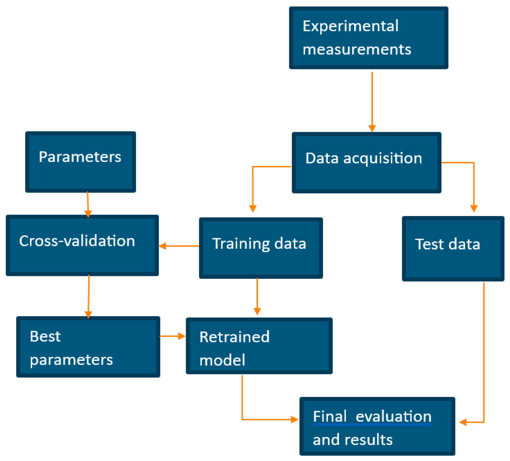
The main goal of the current research work is to provide battery modeling to assess operating mechanisms in the charging and discharging processes, all to optimize Health and Charge estimations based on Remaining Useful Lifetime (RUL) through regression algorithms and binary classifiers. The corresponding steps of the research work are summarized in the following schema, which is illustrated in Figure 1.

The rest of the paper is organized as follows: In Section 2, the problem statement and the motivation of this research are explained. Section 3 describes and implements the methodologies, focusing on Feature Engineering and Exploratory Data Analysis. Section 4 provides the results based on binary classifiers and regression algorithms within the framework of BESSs. Finally, in Section 5, a conclusion is provided to encourage the continuation of this work based on more advanced methodologies to achieve fault diagnostics and predictive maintenance.

2. Data Acquisition and Materials

Lithium-ion cells have become ubiquitous in modern technology and are extensively used in portable electronic devices, electric vehicles, and renewable energy systems due to their high energy density, low self-discharge, and long cycle life. Achieving optimal performance and ensuring the safe operation of these cells demands accurate measurement of their charging and discharging behavior. The charging and discharging curves of a lithium-ion cell provide valuable insights into its capacity, efficiency, voltage, and current profiles.

To ensure precise measurement of the charging and discharging curves of a lithium-ion battery module, a high-accuracy data analyzer was employed. The data analyzer was connected directly to the battery module (which consisted of 16 lithium-ion cells) for voltage measurement and via a current shunt to measure the current. Each cell voltage and current were measured independently. A charging and discharging current of 1/10 C were chosen to obtain reliable data. The measurements were carried out in a closed room with an ambient temperature of 20 °C. Specifications of the battery module datasheet are presented in

Table 1. Battery module datasheet.

Parameter	Value
Width	300.0 mm
Thickness	37.8 mm
Height	127.0 mm
Nominal capacity	218 Ah
Working voltage	2.8–4.35 V
Internal resistance	0.35–0.45 mΩ
Nominal discharge current	72.7 A
Maximum Pulse Discharging	500 A
Cell count	16

.

3. Methods

Initially, Feature Engineering and Exploratory Data Analysis (EDA) are executed to obtain several KPIs related to the SOC, which are based on the Full Equivalent Cycles (FECs). Subsequently, hyperparameter tuning and cross-validation are applied to optimize the mechanism of binary classifiers and regression algorithms. Linear Regression, Ridge Regression, and Lasso Regression are described and executed to estimate the SOH according to the remaining number of cycles extracted from the battery.

Feature Engineering and Exploratory Data Analysis

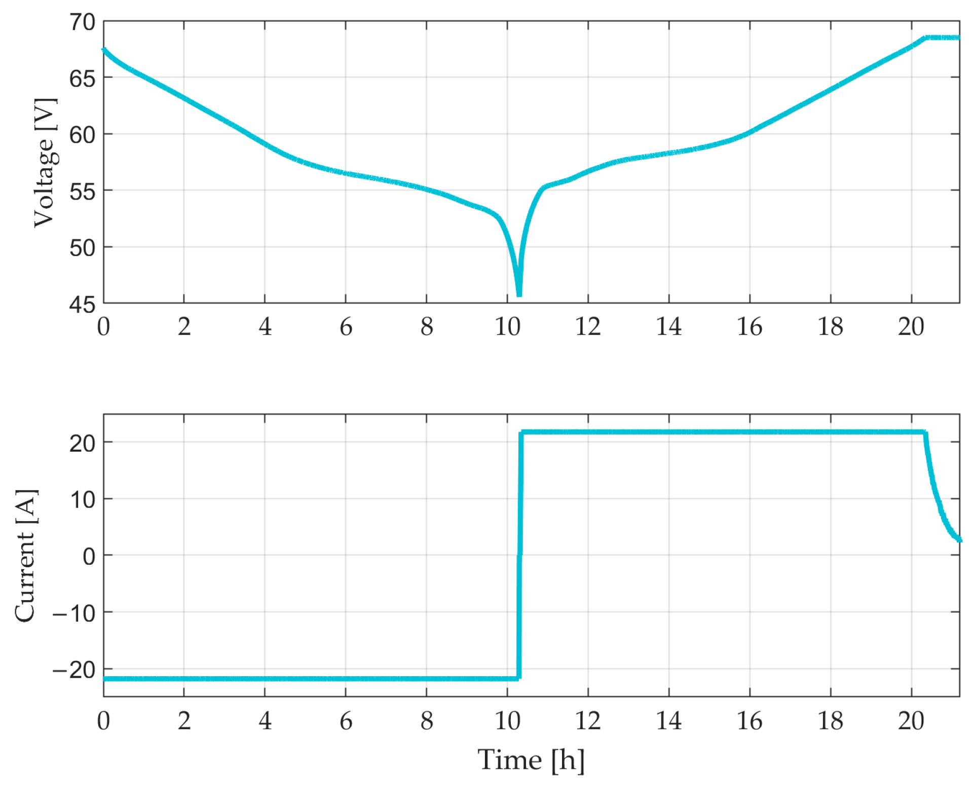
The dataset is processed and sorted based on the operating time, which is represented by charge and discharge. Null values and outliers are searched to ensure a good quality of the experimental measurements before implementing the battery modeling. Initial plots are shown in Figure 2.

In this specific case, before starting EDA, it is necessary to execute Feature Engineering to calculate the required KPIs related to both charge and discharge, all to obtain the FECs that the given battery has undergone, taking into consideration the charge status, charge current, change charge, and several cycles. The following points summarize the Feature Engineering algorithm that calculates the FECs of the battery:

• The SOC is calculated using the Coulomb counter and the input features. After that, the charge status is initially defined according to the SOC and updated throughout the complete process for each iteration. The value is negative if discharged and positive if charged.
• A charge current is defined as a new feature and initialized in the entire process. This variable gives the difference while charging and has a zero value when the battery is in discharge.
• The fraction of completed cycles is calculated based on the positive charge status of the battery and its time evolution.
• The total FECs are calculated considering the cumulative charge status of each iteration. Finally, the capacity, also known as the change of charge per cycle at a given time is obtained by mathematically multiplying the charge current by time.

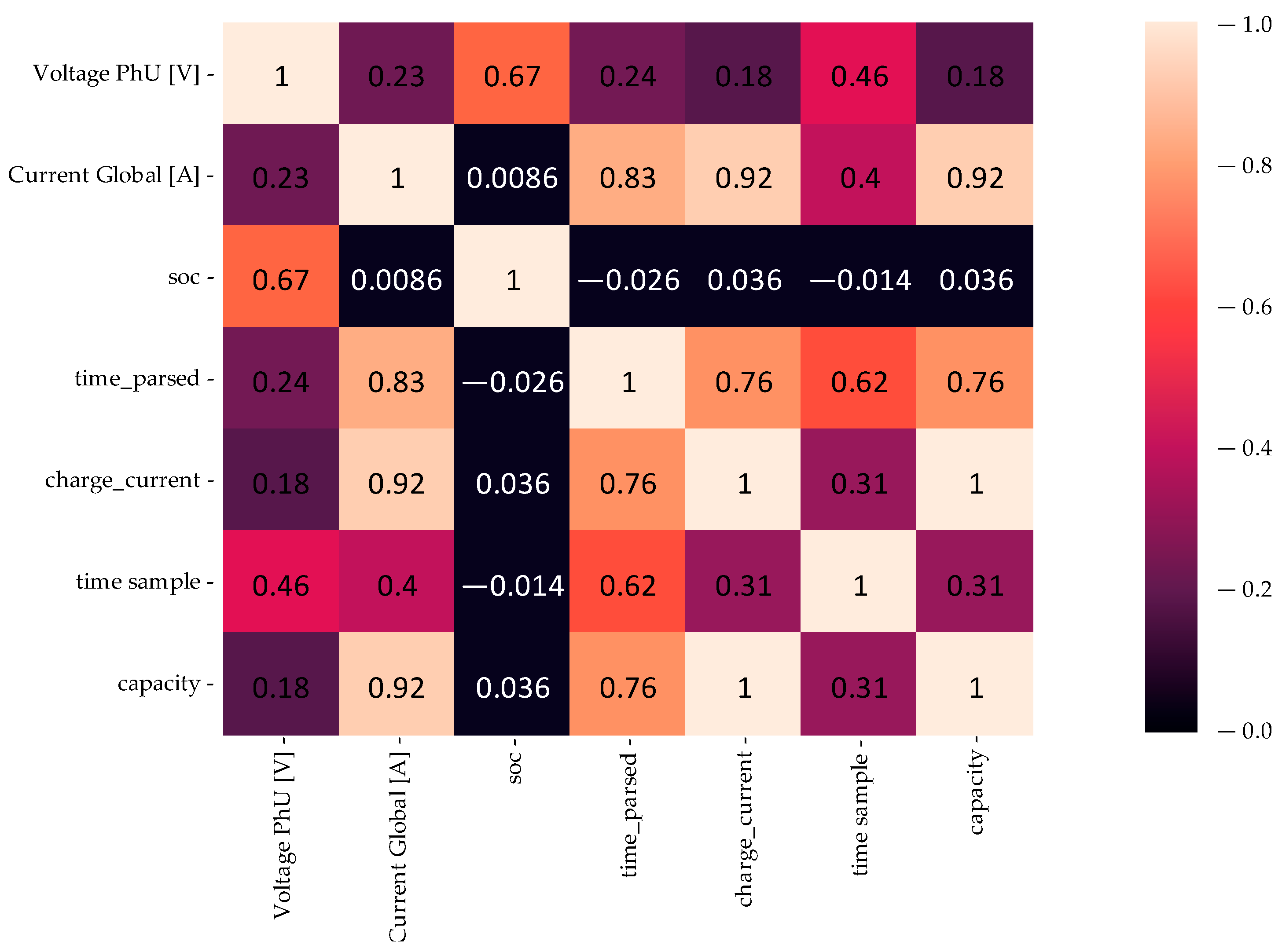
Regarding the contribution of the KPIs, EDA is executed to illustrate the correlation between the newly generated features in the dataset; however, because of the mutual dependence on the charging process, only the most relevant variables are analyzed in the SOC. Visualization of the correlation matrix is illustrated in Figure 3.

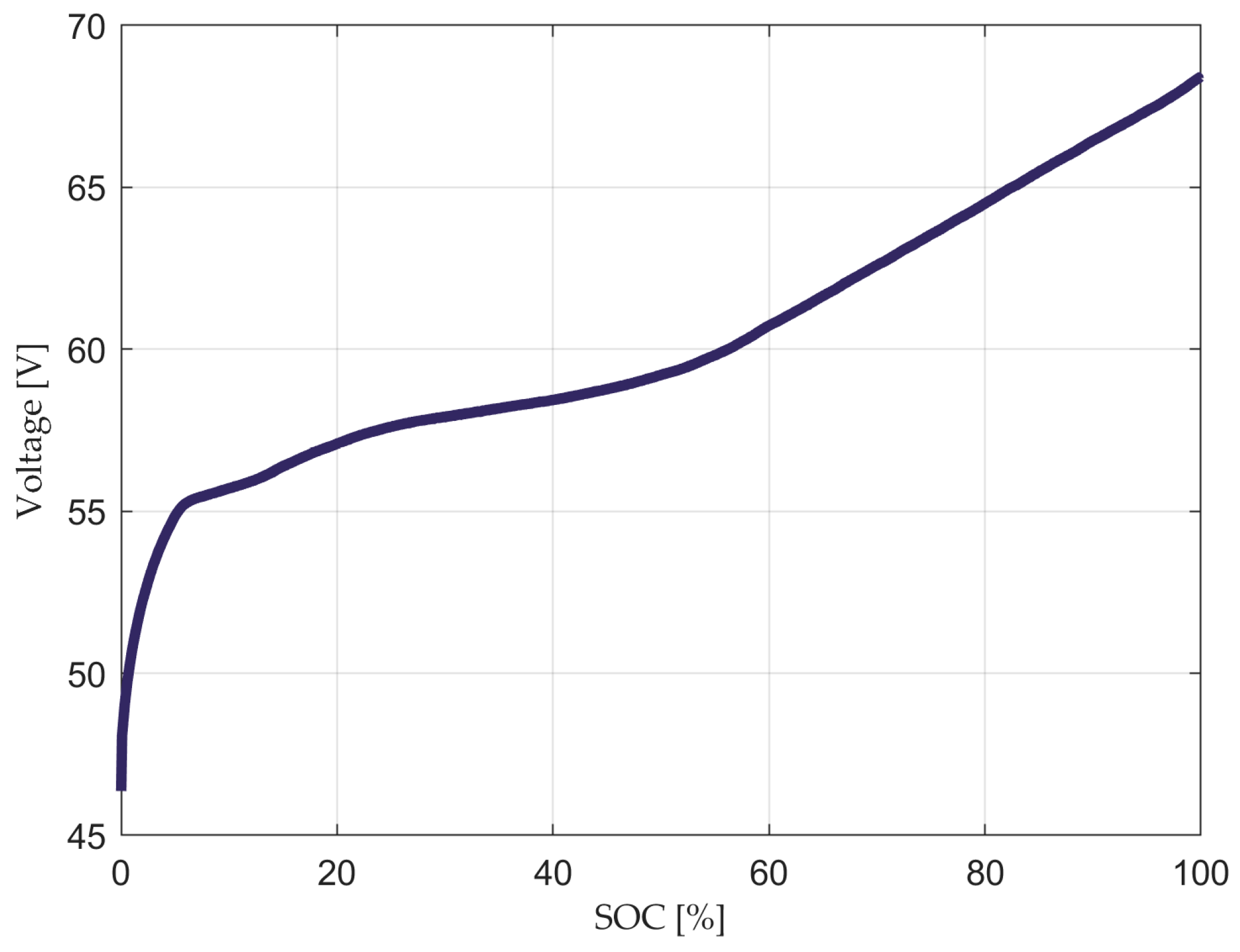
The results indicate that there is a high correlation between the current, time, capacity, and charge current, all due to the Feature Engineering process performed in the previous steps, which is also complemented by the SOC estimations, as expected, showing a mutual dependency of the features SOC vs. time, current vs. capacity, and voltage vs. SOC. The complete charging process is represented by the voltage vs. SOC curve shown in Figure 4 by the SOC and voltage evolution.

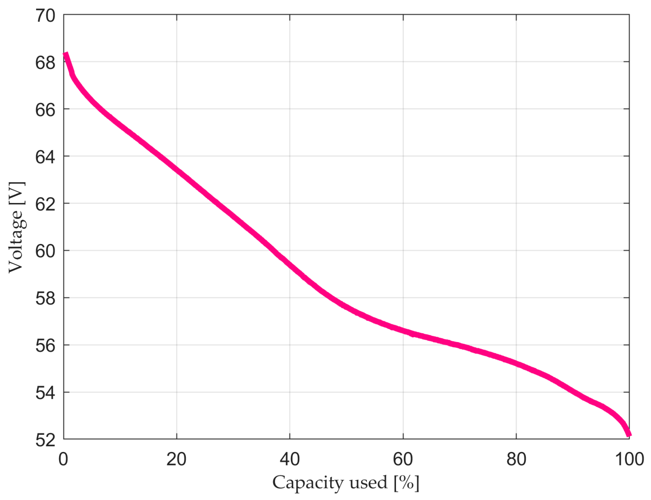
In the discharging process, capacity is the main feature to analyze, all due to the estimations of SOH that will be explained in Section 4. The most relevant insights found in the dataset correspond to the linear relationship between the cycles calculated in the Feature Engineering process and the decrease in capacity, which is a potential indicator to implement regression algorithms for RUL estimations. Figure 5 shows the discharging process in terms of the remaining battery capacity.

Usually, the End-of-Life (EOL) criteria are reached when the capacity of a BESS is lower than 70–80% of the total rated capacity [2]. A graphical representation of the EOL criteria is represented in Figure 6 and reference [6] is used as a basis to illustrate. It is fundamental to point out that the cycle index represents the FEC count of the battery during the discharging process.

4. Results

In this section, binary classifiers and regression algorithms are implemented in the dataset after performing Feature Engineering and EDA. In the first method, the objective is to predict the output variable, which in this specific problem is the profile status: either charge or discharge. Regarding regression algorithms, the goal is to implement a model that estimates the capacity of the battery based on the SOH to calculate the RUL at any given time or cycle.

4.1. Binary Classifiers

Naïve Bayes, Decision Tree, and Logistic Regression are the selected binary classifiers to perform the predictions for the charge and discharge of a battery. It is important to point out that the main purpose of this section is to implement an algorithm that optimizes the operation of the battery by identifying the profile status of the independent variables so that estimations of the SOC and SOH can be automatically performed.

Decision Tree is a Machine Learning algorithm commonly used for classification problems, usually based on developing predictions for a target variable. This algorithm is defined as non-parametric and consists of nodes and branches as principal components, while splitting, stopping, and pruning are model-building steps. Using Decision Tree is considered a potential methodology with several advantages, such as feasible interpretation and understanding, outlier robustness, a non-parametric approach that can deal without considering distributional assumptions, and a simplicity of complex relationships between input and output variables [7].

Logistic Regression is a supervised Machine Learning technique implemented for binary classification problems when the predicted variable is considered categorical. Mathematically, it is based on a logistic function with the purpose of modeling a binary output variable whose range is bounded between 0 and 1, the latter being the main difference compared to Linear Regression. It is necessary to mention that Logistic Regression uses a loss function defined as Maximum Likelihood Estimation (MLE), which is defined as a conditional probability. The advantages of Logistic Regression are the ease of implementation and satisfactory performance achieved with linearly separated classes. Mathematical foundations can be found in references [8,9].

Naïve Bayes is a probabilistic methodology that predicts the classification of a specific target variable described by a set of feature vectors. The mathematical basis corresponds to the Bayes theorem, in which prior distribution is updated into posterior based on empirical information. Naïve Bayes assumption is computed by a likelihood calculation that considers conditional independence between the features and a given class label. Like Logistic Regression, this algorithm implements the MLE to estimate the probabilistic parameters and predict the classification output. It has been demonstrated that Naïve Bayes achieves meaningful results in practical applications, such as systems performance management, text classification, medical diagnosis, etc. [10].

To start the implementation of the binary classifiers, the dataset was labeled according to the profile status, either charge or discharge. After that, two approaches were considered to assess the most accurate and optimal methodology during battery operation. In this target output, the profile status is considered 1 when the battery is charged and 0 if it is discharged; however, it is fundamental to avoid confusion with the charge status performed in the Feature Engineering process, in which the charge current values are updated based on the charge change for each iteration. The following steps summarize the computational algorithm:

• The dataset is processed, and the vector of classes is generated based on the profile status, either charge or discharge, which is defined as the target variable.
• Two approaches are considered to start the implementation of the binary classifiers; therefore, separated arrays are generated. The first approach consists of taking the initial features (i.e., current and voltage) as the independent variables, while the second approach considers the KPIs generated in the Feature Engineering process.
• In each separated array, all features and target variables are randomized to provide the algorithm with a more complex dataset that the binary classifiers will process automatically. It is necessary to point out the importance of this step to avoid processing unbalanced datasets that easily identify patterns to make wrong predictions in later steps.
• Datasets are divided into training and testing. Validation of each binary classifier is executed in a training set through Nested and Non-Nested Cross-Validation [11]. Five-fold cross-validation for inner and outer loops is selected using 30 trials.
• Validation methods are compared, and finally each binary classifier is applied to the testing set to make predictions. Different metrics are calculated to show the performance.

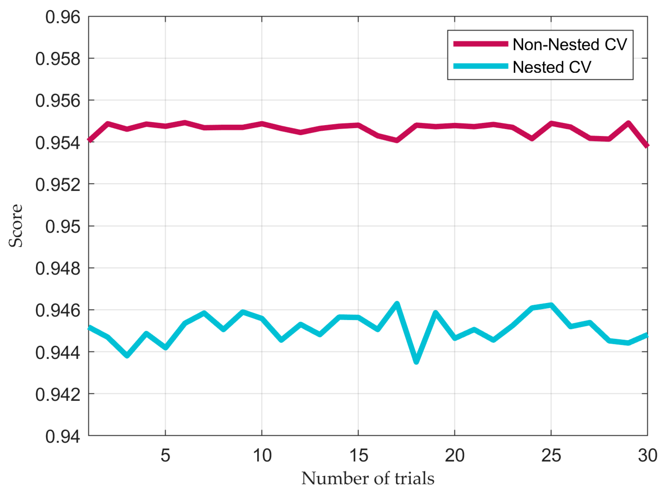
The cross-validation score measures the initial performance of the model, such that the training set is split into a selected number of folds to validate the same model multiple times on different training and validation sets. While Nested-Cross Validation performs feature selection and hyperparameter tuning to select the best combination, Non-Nested Cross-Validation considers a set of parameters previously selected by the user. The results of the Nested and Non-Nested Cross-Validation process for each binary classifier are illustrated in Figure 7, in which different scores were obtained in 30 trials.

It can be appreciated that in this problem, the results of the Non-Nested cross-validation are more optimistic; however, relying solely on the information process and initial dataset without implementing Feature Engineering might result in a biased classification model. According to the cross-validation score in the training dataset, binary classifiers show a significant level of performance, which should be in the same range as the test set when evaluating final performance metrics.

In a classification problem, the accuracy of the model refers to the total observations, considering both positive and negative, that were correctly predicted. Sensitivity, also known as True-Positive Rate, refers to all positive observations that are correctly classified as positive. Specificity is defined as the True-Negative Rate, which measures the total observations accurately predicted as negative [12].

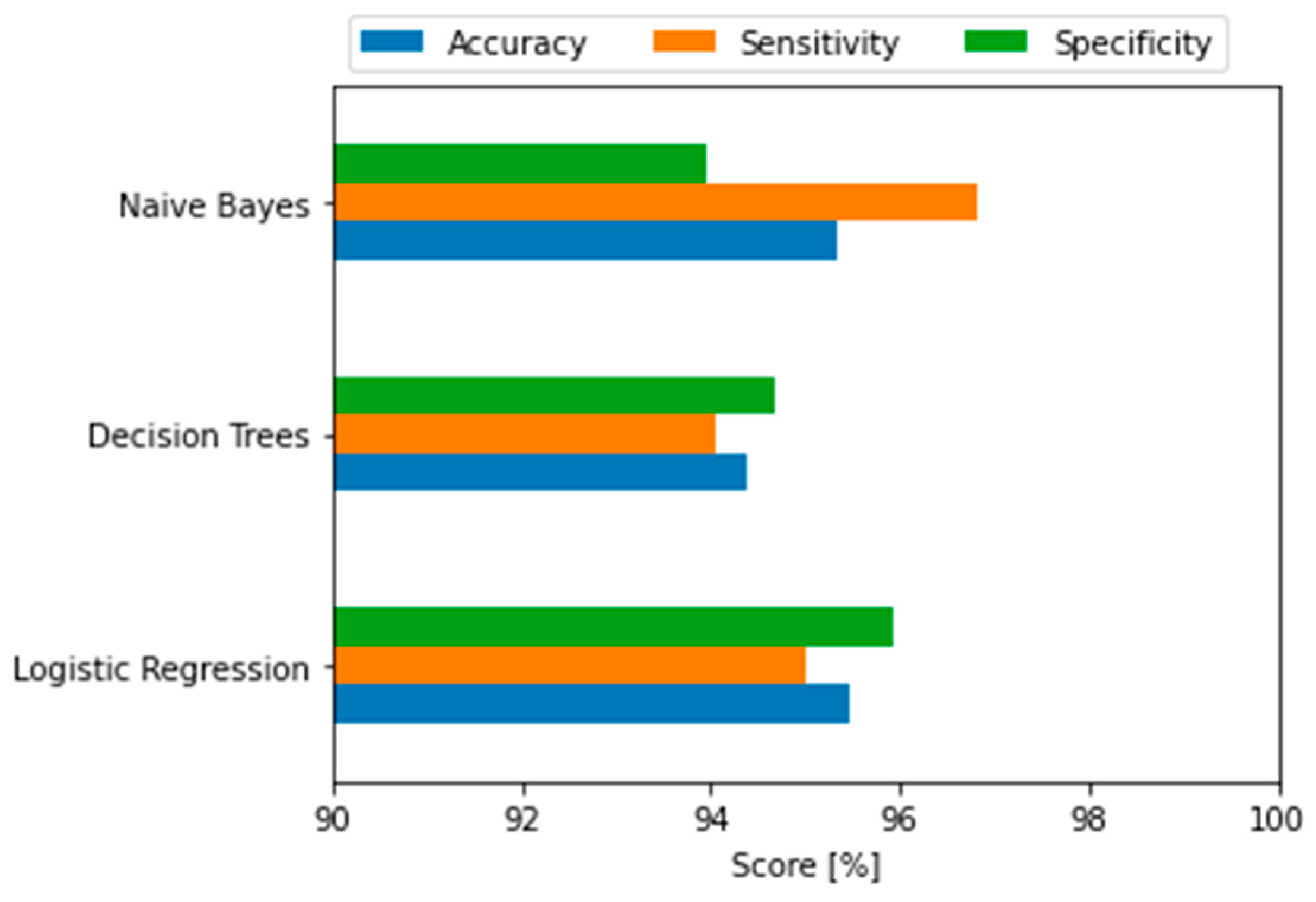
Both approaches previously described in the computational algorithm were implemented using Naïve Bayes, Decision Tree, and Logistic Regression. Regarding the performance metrics to evaluate that of each classifier, precision, sensitivity, and specificity are calculated and plotted in Figure 8, demonstrating a high score that is in a similar range compared to the cross-validation process.

The final performance for each binary classifier shows that accuracy is around 95%, and sensitivity corresponds to a value close to 96%. On the other hand, the specificity has a slightly smaller difference, of 94%, compared to previous metrics for Naïve Bayes and Decision Tree. A detailed analysis of the above results will be provided at the end of this section.

4.2. Regression Algorithms

Linear Regression is considered one of the most widely used models in Machine Learning. Mathematically, it finds linear coefficients and deals with the prediction of continuous numeric outcomes. In the context of regression, the terminology “linear” refers to a model in which a dependent variable has a relationship expressed as a linear combination of independent variables. Additionally, linear methods can be applied to the transformation of the inputs, usually called basis function methods [13].

Overfitting is considered one of the most common problems when implementing Machine Learning estimations and is based on retaining a subset of the predictors and discarding the rest, which produces a high variance that consequently reduces the prediction error of the full model. Probable causes of overfitting may be the fact that the chosen model structure and data do not conform, so shrinkage methods are applied to overcome this problem. Regularization is defined as a shrinkage method that imposes a penalty on the cost function and prevents larger values of the estimated coefficients, with Ridge and Lasso (Least Absolute Shrinkage and Selection Operator) Regression being remarkable shrinkage methods that do not suffer as much from high variability [13].

Ridge Regression is a shrinkage technique used when the independent variables have an elevated level of correlation, also known as multicollinearity. In Ridge Regression, a shrinkage parameter is added to achieve a low variance that minimizes a penalized sum of squares and reduces the standard errors, all by adding the squared magnitude of the coefficients to the cost function. [13]. However, instead of using squares, Lasso Regression uses absolute values as a penalty of the coefficients to the loss function. Like Ridge Regression, Lasso Regression also reduces the variability and improves the performance of Linear Regression; however, when a group of predictors shows an elevated level of multicollinearity, one of them is selected and shrinks the others to zero, making it a technique useful in feature selection [14].

In this subsection, the BESS capacity and discharging cycles are analyzed to calculate the SOH, which is defined as the output or target variable in the methodology. Finally, regression algorithms are executed to estimate the RUL before reaching the EOL criteria and to predict the SOH based on the previous calculated values. The methodology is explained as follows:

• The cycle indexes and the discharge capacity are considered as input variables. After that, each cycle is updated according to the capacity values associated with every time step.
• The SOH is calculated considering the initial capacity of the BESS and its discharging evolution through every cycle. The cycles and BESS capacity are defined as the predictors, whereas the SOH is considered the predicted variable to initialize the regression algorithms.
• The data are divided into training and testing. In this step, Linear, Ridge, and Lasso Regression are implemented.
• Cross-validation is executed in a training set to compare the performance of the Linear Regression and regularization techniques. Cross-validation scores are obtained and the most optimal hyperparameters of the regularization methods are selected to build and test the final models.
• The RUL is estimated, and the performance of each regression algorithm is evaluated by calculating the Mean Squared Error (MSE), Mean Absolute Error (MAE), and coefficient of determination ($R^2$).

The initial results indicate that by implementing Linear Regression, the performance of the model is slightly higher compared to the regularization methods; however, as previously mentioned, overfitting may occur in the testing process, so that shrinkage techniques are recommended to obtain a more stable and reliable model.

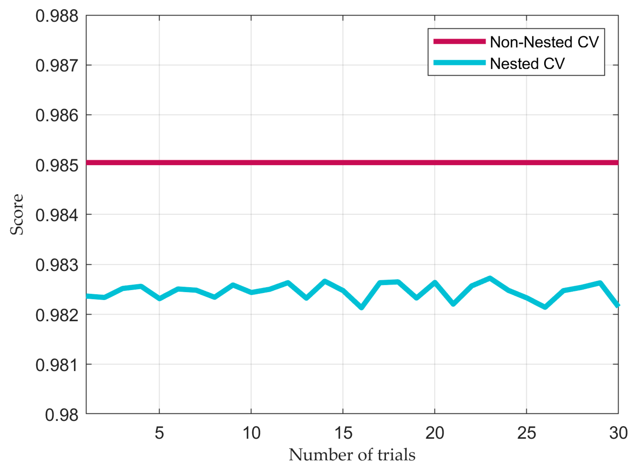
Like binary classifiers, cross-validation is used to validate the model, specifically to note the difference in performance using regularization in the regression algorithms. Nested Cross-Validation has been used to optimize the selection of hyperparameters for Lasso and Ridge Regression; however, in the case of Linear Regression, Non-Nested Cross-Validation uses the same data to fit model parameters and assess model performance. The cross-validation score process is illustrated in Figure 9, which compares the performance with and without regularization.

A constant value of the Linear Regression score in the cross-validation step indicates that hyperparameter tuning is not applicable; on the other hand, regularization methods show a different performance due to optimized hyperparameter tuning, which is explained by the shrinkage parameters, providing a performance in the range of 97%. It is crucial to mention that, as indicated in the previous subsection, the final performance of the regression algorithms must not differ substantially from the cross-validation process.

Finally, the performance of each regression algorithm is evaluated in the testing. The numerical results of the MSE, MAE, and $R^2$ are shown in

Table 2. Performance of different regression algorithms.

Regression	MSE	MAE	${\mathit{R}}^{\mathbf{2}}$
Linear	0.0155	0.0119	0.9779
Ridge	0.0153	0.0110	0.9768
Lasso	0.0188	0.0153	0.9650

.

All the regression algorithms show a similar performance in the testing step, corroborating the cross-validation process; however, compared to Linear Regression, the regularization methods provide a more optimal performance in the case of multicollinearity between the independent variables in the dataset, which in this specific problem prevents not only overfitting, but also a possible bias due to model simplicity or erroneous assumptions.

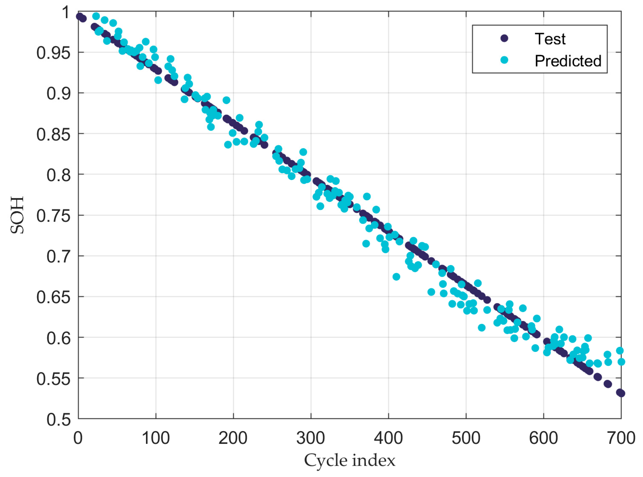
Figure 10 illustrates the implementation of the regression algorithms, comparing the testing and predicted results of the SOH during the BESS’ operation.

It is fundamental to point out that points graphically close to the straight line indicate a high-quality level in the implementation of the regression algorithms. In addition, the predictions of SOH values after the EOL criteria are illustrated to show the robustness of the algorithms across the entire dataset, all because considering a significant sample of data points prevents easy predictions, which may result in overfitting due to high variance and low bias.

Regarding the RUL results,

Table 3. RUL results considering cycles and SOH.

Cycle	RUL	SOH
50th	396 cycles	0.9695
200th	246 cycles	0.8650
300th	146 cycles	0.7780
400th	46 cycles	0.7283

provides the SOH and the corresponding cycles. As shown in Figure 10, the battery reaches 70% of SOH in cycle 446.

5. Discussion

Hyperparameter tuning and cross-validation play a key role in implementing BESS modeling and achieving accurate estimations of the target variable, all because of the different KPIs and level of mutual correlation. Furthermore, Feature Engineering is a helpful process that can provide promising insights not only to analyze the dataset, but also to obtain a new subset of features in the charge and discharge of a BESS.

Regarding the binary classifiers, the approach that consists of taking the voltage and current as input features showed an elevated level of performance metrics, which is supported by the fact that constant values of current during the charge and discharge represent a potential trend to predict the binary output. The second approach, which considers the KPIs generated in the Feature Engineering process, showed slightly lower but optimistic performance compared to the first approach, and it is concluded that although input features are randomized to avoid easily processing patterns for unbalanced datasets, multiple BESS indicators must be provided to achieve performance metrics at the same numerical level for sensitivity, specificity, and accuracy. Logistic Regression and Decision Tree achieved a prominent level of performance metrics that is not dependent on the quantity of selected features, all because of the hyperparameter tuning, however, Naïve Bayes provided a lower specificity by considering the KPIs generated in the Feature Engineering process, being the assumption of independence features a cause.

Finally, regression algorithms provided a similar performance in the cross-validation and testing steps, demonstrating the promising results of the BESS modeling based on the RUL. Compared to the binary classifiers implementation, hyperparameter tuning and cross-validation do not manifest computational expensive outputs, which is explained by a lower quantity of predictors. In this approach, the quantity of cycles, discharging capacity, and the calculated SOH are the indicators of a mathematical relationship that fits a linear model, which can also be implemented in more advanced research approaches that consider the external degradation mechanisms during the operation of a BESS.

6. Conclusions

The article examined and measured a battery module comprising 16 cells, resulting in the acquisition of charging, and discharging curves. Binary classifiers and regression algorithms are described, analyzed, and implemented to assess the BESS based on Health and Charge indicators. The statistical results achieve a validation and testing accuracy of 96% and 95% for binary classifiers, while 98% and 97% corresponding to regression algorithms. The research work aimed to familiarize the reader with the importance of BESS operation according to the profile status and EOL criteria through Machine Learning. Regarding the implementation of both regression and binary classifiers, hyperparameter tuning and cross-validation must be considered to achieve optimal metrics of performance. Thus, the first step is to become familiar with the mathematical foundations of the computational algorithm to explain the behavior of the dataset in a battery.

The main contribution of this research work is providing an initial methodology for estimating Health and Charge indicators in a BESS through binary classifiers and regression algorithms. The novelty associated with the proposed methods is the implementation of robust computational algorithms that not only automatically classify the profile status of a BESS, but also perform data science techniques to optimize the modeling during battery operation. Innovative techniques are summarized to obtain helpful insights about the KPIs in a BESS, all to demonstrate that promising results can be obtained when computer science techniques are implemented under the framework of renewable energy technologies.

Finally, the data-driven approaches discussed in this article correspond to validated methodologies that the scientific community has implemented for different types of problems, BESS being one of the most important to achieve the energy transition. Furthermore, different datasets must be processed to evaluate the lifetime operation of a BESS, specially to test battery cells and design diagnostics methodologies; however, it is important to mention that external factors must be considered to build several types of models, such as thermal conditions, mechanical degradation, vibrations, etc. This work is the basis for designing a methodology for the diagnostics of BESSs through Machine Learning network architectures by the utilization of Explainable Artificial Intelligence methods. Moreover, this work provides a research environment for battery management in digital twin and electric vehicle applications to test and compare the performance of diverse types of battery modeling. This will help to establish assessment and verification procedures for fault diagnostics to support commercial consulting, research, and testing for enterprises based on the digital twin concept.

References

- Liao, C.; Li, H.; Wang, L. A dynamic equivalent circuit model of LiFePO4 cathode material for lithium ion batteries on hybrid electric vehicles. In Proceedings of the 2009 IEEE Vehicle Power and Propulsion Conference, Dearborn, MI, USA, 7–10 September 2009; pp. 1662–1665. [Google Scholar] [CrossRef]
- Rahn, C.D.; Wang, C.-Y. Battery System Engineering; John Wiley & Sons, Ltd.: Hoboken, NJ, USA, 2013. [Google Scholar]
- Pop, V.; Bergveld, H.J.; Notten PH, L.; Regtien, P.P. State-of-the-Art of Battery State-of-Charge Determination; Measurement Science and Technology; Springer: Dordrecht, The Netherlands, 2005; Volume 16, pp. 93–110. [Google Scholar]
- Berecibar, M.; Gandiaga, I.; Villarreal, I.; Omar, N.; Van Mierlo, J.; Van den Bossche, P. Critical review of state of health estimation methods of Li-ion batteries for real applications. Renew. Sustain. Energy Rev. 2016, 56, 572–587. [Google Scholar] [CrossRef]
- Meng, J.; Azib, T.; Yue, M. Early-Stage end-of-Life prediction of lithium-Ion battery using empirical mode decomposition and particle filter. Proc. Inst. Mech. Eng. Part A J. Power Energy 2023, 2023, 09576509231153907. [Google Scholar] [CrossRef]
- Macintosh, A. Li-Ion Battery Aging Datasets. Ames Research Center. 2010. Available online: https://c3.ndc.nasa.gov/dashlink/members/38/ (accessed on 24 April 2023).
- Song, Y.; Lu, Y. Decision tree methods: Applications for classification and prediction. Biostat. Psychiatry 2015, 27, 130–135. [Google Scholar]
- Peng, C.Y.; Lee, K.L.; Ingersoll, G.M. An Introduction to Logistic Regression Analysis and Reporting. J. Educ. Res. 2002, 96, 3–14. [Google Scholar] [CrossRef]
- Belyadi, H.; Haghighat, A. Machine Learning Guide for Oil and Gas Using Python; Gulf Professional Publishing: Woburn, MA, USA, 2021; Volume 1, pp. 169–295. [Google Scholar]
- Rish, I. En Empirical Study of the Naïve Bayes Classifier; T.J. Watson Research Center: Hawthorne, NY, USA, 2001; pp. 41–46. [Google Scholar]
- Berrar, D. Cross-Validation. In Encyclopedia of Bioinformatics and Computational Biology; Elsevier: Amsterdam, The Netherlands, 2018; Volume 1, pp. 542–545. [Google Scholar]
- Foody, G.M. Status of land cover classification accuracy assessment. Remote Sens. Environ. 2002, 80, 185–201. [Google Scholar] [CrossRef]
- Murphy, K.P. Machine Learning: A Probabilistic Perspective; The MIT Press: Cambridge, MA, USA, 2012. [Google Scholar]
- Hastie, T.; Tibshirani, R.; Friedman, J. The Elements of Statistical Learning: Data Mining, Inference, and Prediction, 2nd ed.; Springer Series in Statistics; Springer: Berlin/Heidelberg, Germany, 2017. [Google Scholar]