Featured Application
The findings of this study can be applied in the design and experimental investigation of line-start permanent magnet motors.
Abstract
Line-start permanent magnet synchronous motors (LSPMSMs) are of great interest to researchers because of their high energy efficiency, due to the growing interest of manufacturers in energy-efficient units. However, LSPMSMs face some difficulties in starting and synchronization processes. The LSPMSM lumped parameter model is applicable to estimating the successfulness of starting and further synchronization. The parameters of such a model can be determined using computer-aided identification algorithms applied to real motor transient processes’ curves. This problem demands significant computational time. A comparison between two algorithms, differential evolution and Nelder–Mead, is presented in this article. The algorithms were used for 0.55 kW, 1500 rpm LSPMSM parameter identification. Moreover, to increase computational speed, it is proposed to stop and restart the algorithms’ procedures, changing their parameters after a certain number of iterations. A significant advantage of the Nelder–Mead algorithm is shown for the solving of the considered problem.
1. Introduction
A significant share of industrial mechanisms, including pumps, fans, air blowers, and compressors, are driven by electric motors, which are connected directly to a power grid without intermediate power converters and are launched using a direct start [1,2,3]. The vast majority of these motors are induction motors (IMs) [1,2,3]. Despite all the well-known induction motors’ advantages, they expose significant losses during the rotor winding, which diminishes their energy efficiency class [4].
Line-start permanent magnet synchronous motors (LSPMSMs) do not have noticeable rotor winding losses at steady state, which increases their energy efficiency class in comparison to induction motors. LSPMSMs are available on the market and mostly are employed in pump and fan units [5,6,7]. Figure 1 shows a comparison of IM and LSPMSM designs.
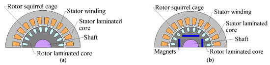
Figure 1.
Sketches of electric motors. (a) Induction motor (IM); (b) synchronous motor with the direct start from the network and permanent magnets (LSPMSM).
LSPMSMs are of great interest to researchers because of their high energy efficiency due to the growing interest of manufacturers in energy-efficient units [8,9,10,11]. The LSPMSM model’s performance can be improved by using computer-aided design optimization procedures [12,13,14].
There are studies investigating LSPMSM performance at unbalanced voltage [15]. In [16], the LSPMSM steady-state torque was evaluated by transient analysis using a neural network. Article [17] is devoted to LSPMSM modelling, using a bond graph model [18]. Article [19] discusses the latest LSPMSM design techniques. Article [20] presents an experimental comparison of a 4-pole 5.5 kW LSPMSM with axial and radial fluxes. There are also studies on the effect of LSPMSM rotor design on additional losses [21].
LSPMSMs face some difficulties in starting and synchronization processes, especially with loads with a high moment of inertia [22,23,24]. An LSPMSM lumped parameter model [25] was applied to estimate the successfulness of starting and further synchronization, which has been extremely beneficial for the experimental verification of LSPMSM characteristics. However, experimental parameter identification is related to significant obstacles.
Evaluation of electrical parameters can be done using a finite element model (FEM) based on known motor constructive parameters [26]. However, this approach requires knowledge of the geometrical details of the motor core, winding data, and the materials it is composed of. This requires access to motor design documentation or irreversible disassembly of motor parts for study purposes, which is not always possible.
In the case that the motor constructive parameters are unknown, there are several approaches for determining equivalent circuits parameters applicable for IMs [27,28,29,30,31,32,33] and LSPMSMs [25,26,34,35]: (1) steady-state experiments, such as no-load tests, locked rotor tests, etc., allow individual motor parameters to be determined [25]; (2) computer-aided identification algorithms make it possible to use the transient response to estimate multiple motor parameters, as explained in [34].
Measurement techniques of individual LSPMSM parameters using steady-state experiments include: the stator winding DC resistance estimation; the leakage inductance estimation on sinusoidal voltage operation with rotor extraction; the locked rotor test for rotor resistance and inductance estimation; the DC step-voltage test to estimate the LSPMSM total inductances; and the open-circuit test used for the permanent magnet flux linkage estimation [25]. However, such an approach demands a very high measurement accuracy and relies on many assumptions. The presence of the mutual inductance of the stator winding and the rotor squirrel cage makes it impossible to measure the total inductances at a locked rotor. Further, the total inductances measurement using the DC step-voltage test has low accuracy because of the nonlinear nature of the motor total inductances, which is the result of the presence of main-path saturation and cross saturation in the motor magnetic circuit.
According to Newton’s second law, the rotor moment of inertia can be measured as a coefficient between dynamic torque and angular acceleration. However, it demands a laboratory test bench with a prime mover and a torque sensor or a frequency converter with a specific testing algorithm, which are not always available [36].
These difficulties can be overcome by computer-aided identification methods that require only phase currents and speed measurement during the motor start-up process.
There are many computer-aided identification algorithms; for example, the Kalman filter, the model reference adaptive system, the least squares method, artificial neural networks, the genetic algorithm, the differential evolution algorithm, particle swarm optimization, etc. [27,34,35]. For example, in [34], the identification of LSPMSM parameters based on the time plots of current and speed during start-up using the differential evolution algorithm is discussed.
It can be concluded that, due to the disadvantages of other methods, such as the need to know the motor design parameters in the case of using FEA or a large number of assumptions in the case of parameter estimation through steady-state experiments, computer identification is a promising method for estimating the parameters of the LSPMSM model. However, a detailed comparison of the effectiveness of various computer identification algorithms for determining the parameters of LSPMSM has not yet been carried out.
This article presents a comparison between the differential evolution (DE) [37,38] and Nelder–Mead (NM) algorithms [39,40] for lumped parameter LSPMSM model identification. The novelty of this article lies in the results of comparing the DE and NM algorithms for the considered specific problem. Moreover, it shows the advantages of the NM algorithm over the DE algorithm. Its practical impact lies in revealing a more accurate and computationally efficient algorithm for the identification of LSPMSM parameters.
The comparison was carried out on the example of transients calculated for the LSPMSM model with given parameters. The results of the study show that the differential evolution algorithm demonstrates relatively low parameter identification accuracy and longer computational time. However, it can be used to determine the initial approximation for the algorithms with better convergence. The Nelder–Mead algorithm is confirmed as more computationally efficient for the considered problem.
Moreover, it is proposed to stop and restart identification procedures for both algorithms, changing their tuning parameters, when the rate of convergence shows a significant decrease.
The purpose for identifying the parameters of the LSPMSM in our study is to obtain a tool that correctly predicts the success/failure of starting and synchronizing the LSPMSM for various moments of inertia and for the various dependencies of the load torque on the speed. We have added this explanation to the article.
2. Mathematical Model of the Motor
The transient processes for the LSPMSM start-up are calculated using the LSPMSM mathematical model.
When modelling the LSPMSM, it is assumed that:
- The magnetic fields generated by the stator and rotor windings have a sinusoidal spatial distribution;
- The magnetic permeability of the steel is constant;
- The stator and rotor windings are symmetrical;
- Each winding is powered by a separate source;
- The mains voltage phasor is constant throughout the entire starting process, and an increase in the motor current does not cause a decrease in its amplitude;
- The magnetic core losses are not taken into account.
The system of ordinary differential LSPMSM equations to be solved is represented as:
where Usd and Usq are the stator voltages along the d and q axes; Isd, Isq, I′rd, and I′rq are the stator and rotor currents; Lsd, Lsq, Lrd, and Lrq are the stator and rotor total inductances; Lσd and Lσq are the rotor leakage inductances; λsd, λsq, λ′rd, and λ′rq are the stator and rotor flux linkages; λ′0 is the permanent magnet flux linkage; Rs is the stator resistance; Zp is the number of motor pole pairs; r′rd and r′rq are the rotor resistances; φ is the mechanical rotational angle equal to the integral of the motor speed ω; T is the motor torque; Tload is the loading torque; J is the total moment of inertia. All initial conditions are equal to zero, except for the stator flux along the q-axis λsq 0 = λ′0.
dλsd/dt − p·λsq·dφ/dt + Rs·Isd = Usd;
dλsq/dt + p·λsd·dφ/dt + Rs·Isq = Usq;
dλ′rd/dt + r′d·I′rd = 0;
dλ′rq/dt + r′q·I′rq = 0;
I′rd = (λ′rd − λsd)/Lσd;
I′rq = (λ′rq − [λsq − λ′0])/Lσq;
Isd = λsd/Lsd − I′rd;
Isq = (λsq − λ′0)/Lsq − I′rq;
T = 3/2·Zp(λsd·Isq − λsq·Isd);
J·d2φ/dt2 = T − Tload,
dλsq/dt + p·λsd·dφ/dt + Rs·Isq = Usq;
dλ′rd/dt + r′d·I′rd = 0;
dλ′rq/dt + r′q·I′rq = 0;
I′rd = (λ′rd − λsd)/Lσd;
I′rq = (λ′rq − [λsq − λ′0])/Lσq;
Isd = λsd/Lsd − I′rd;
Isq = (λsq − λ′0)/Lsq − I′rq;
T = 3/2·Zp(λsd·Isq − λsq·Isd);
J·d2φ/dt2 = T − Tload,
Figure 2 shows the implementation of equation system (1) in Simulink. According to Figure 2a, the LSPMSM fed directly from the mains (“Discrete 3-phase Source”), was mechanically coupled to the load. The load was simulated as a summation of a constant torque Tc and component ω·F that represented a bearings frictional torque, which depended on speed linearly, as is shown in Figure 3b.
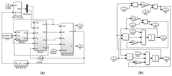
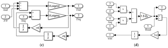
Figure 2.
Simulink model of the LSPMSM motor in the d-q axes. (a) General view of the model; (b) calculation of stator currents; (c) calculation of rotor currents; (d) torque calculation.
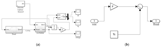
Figure 3.
Simulink model of the LSPMSM motor fed from 3-phase 380 V, 50 Hz grid. (a) General view; (b) load torque model.
The LSPMSM parameters (rated power 550 W, rated speed 1500 rpm) given in Table 1 were taken as the motor parameters.

Table 1.
The LSPMSM parameters (rated power 550 W, rated speed 1500 rpm).
It is known that the operating temperature significantly affects the resistance and rotational speed of induction motors [41]. At the same time, the heating of the LSPMSM is much less due to lower losses, and it does not have any slip. This makes it possible to not consider the influence of temperature when identifying its parameters [34].
Figure 4 represents the LSPMSM phase currents and angular frequency transient processes at Tc = 0 N·m and F = 10−4 N·m/(rad/s). Figure 4a shows the time plots of the components of the stator current along the direct (d) and quadrature axis (q) in a coordinate system fixed relative to the rotor. Figure 4b shows the time plot of the mechanical angular frequency of the rotor. Figure 5 shows the directions of the d and q axes relative to the magnetization direction of the permanent magnets. The transient waveforms were selected for the study because these values (phase currents and angular frequency) can be easily measured in experiments with the real LSPMSMs. Figure 4 shows that the LSPMSM starting time was 0.7 s. The steady-state phase current amplitude was 1.58 A. The starting inrush current was 15.8 A. During the starting process, the motor reached the synchronous speed of 157.09 rad/s (1500 rpm) at 0.06 s for the first time; however, further, it accelerated to a higher speed because of inertia. Later, the motor decelerated as a result of synchronous torque action. These oscillations were repeated several times with the decreasing amplitude caused by dumping factors such as asynchronous torque and load frictional torque.
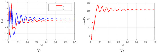
Figure 4.
LSPMSM starting simulation results: (a) d and q-axis stator currents; (b) motor speed ω.
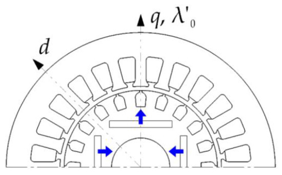
Figure 5.
Axes d and q of the rotor relative to the permanent magnet magnetization direction (indicated by blue arrows).
3. General Algorithm of the Motor Parameters Identification
The flow chart of the motor parameters identification algorithm is shown in Figure 6. It is valid for both DE and NM. During the initialization stage, a set of identifiable parameters, their constraints and initial conditions, parameters of the objective function that do not change during optimization (amplitude and frequency of the supply voltage, number of poles, stator resistance, etc.), as well as a settings identification algorithm (number of iterations, maximum optimization function execution time, coefficients that impact the optimization process, number of individuals in a population for DE, etc.) were defined. Since the Nelder–Mead method is an unconstrained method, the constraints were applied only if DE was used. DE is a bound-constrained global search algorithm that requires setting up quantities and names of the variables, their constraints, and an initial approximation, as well as accuracy if the solving problem demands it.
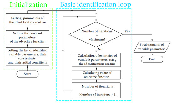
Figure 6.
One-stage identification algorithm flow chart.
In the basic identification loop, using the identification algorithm (DE or NM), the next estimate of the identified parameters was calculated, which was the input of the objective function. In the objective function, the simulation of the Simulink model was called using the function “sim” [42], whose inputs were the name of the model, its initial state, etc., and the output was the vector of simulation results of the Simulink model.
An objective function, Fvalue, that should be minimized during the basic identification cycle was calculated as an integral of the squared deviations of the angular frequency ωm and the currents id and iq for separated time samples, calculated at the current values of the identifying parameters of reference transient processes functions shown in Figure 4:
where kid = 20, kiq = 20 and kω = 1 are the weight coefficients according to [34]; qid, qiq and qω are the error functions. These error functions are defined as follows:
where idm, iqm and ωm are simulation results of the d- and q-axis stator currents and angular frequency, respectively, obtained using motor parameters given in Table 1.
Fvalue = kid · qid + kiq · qiq + kω · qω,
The basic identification loop ended after the specified number of iterations had been completed. The parameter estimate obtained after this was the result of identification.
4. Identification Algorithms
As was stated earlier, the implementation results of the two algorithms (DE and NM) were compared for the LSPMSM parameter identification problem. DE is a multidimensional optimization algorithm which belongs to the stochastic optimization algorithms group. DE is the result of further development of the genetic algorithm [38]. According to the original definition, DE can be described as follows. Initially, a set of vectors called generation is created. N-dimensional points where a minimized objective function f(x) is determined are considered as vectors. The algorithm creates a new generation of randomly combined vectors from the previous generation. The number of vectors is the same for each generation, and this is one of the algorithm parameters.
A new generation of vectors Is generated as follows. For each previous generation vector xi, three different random vectors, v1, v2, and v3, are selected among the previous generation except vector xi itself. As a result, a mutated vector (6) is generated:
where Fv is one of the method parameters, which is a positive real number in the range (0, 2). It is recommended to vary this value when an objective function approaches a minimum [31].
v = v1 + Fv (v2 − v3),
Then, the crossover procedure is implemented on mutated vector v. The procedure consists of the replacement of some of the vector’s coordinates by initial vector xi coordinates. Each replacement is performed with some probability, which is another parameter of the algorithm. The result after the crossover procedure vector is called a trial vector. If this vector is «better» than the initial vector xi, which means that an objective function value was reduced, then xi is replaced by the trial vector in a new generation. Otherwise, the previous xi vector remains as an initial vector.
The NM is an unconstrained optimization algorithm applicable to the function of several variables [40]. The algorithm searches for a local optimum and can «stick» in one of the local optima. Different initial simplex shapes can be changed to find the better minimum if necessary.
The NM is used to find the unconstrained minimum of a function of n variables defined elsewhere in .
The algorithm parameters are listed below:
- -
- Reflection coefficient α > 0.
- -
- Contraction coefficient 0 < β < 1.
- -
- Expansion coefficient γ > 1.
Usually, units α = 1, β = 0.5, and γ = 2 are selected.
The algorithm contains the following steps enumerated to highlight function calls:
Preparation. Initially, n + 1 points are selected: xi = (xi1, xi2, …, xin), i = 1…(n + 1), where x1 = (x11, x12, …, x1n) is an initial parameter vector, x2 = (x11·(1 + δ), x12,…, x1n), x3 = (x11, x12·(1 + δ),…, x1n)…, xn+1 = (x11, x12,…, x1n·(1 + δ)), δ is the initial simplex coefficient. These vectors constitute the n-dimensional space simplex. Objective function values are calculated at the points f1 = (x1), f2 = f(x2),…, fn+1 = f(xn+1).
Sorting. Three points are selected among simplex vertices: xh where function value fh is the greatest, xg where fg is the next to the greatest, and xl where fl is the least function value. The further steps’ aim is at least the diminishing of fh.
A centroid of the aforementioned points of the simplex excluding xh is determined as xc = 1/n ∑(i ≠ h)(xi). Calculation of fc = f(xc) is not mandatory.
Reflection. The reflection xr = (1 + α)xc − αxh of xh with respect to xc with coefficient α and the value of the function fr = f(xr) at xr is to be calculated.
Expansion. Then fr is compared with the values fh, fg, and fl:
If fr < fl, the selected search direction is successful, and the search step can be increased using the expansion operation. A new point xe = (1 + γ) xc − γxr and the function value fe = f(xe) are to be calculated.
If fe < fr, the simplex expands up to this point: set xh equal to xe and fh equal to fe, and then finish the current iteration (go to Step 6).
However, if fr < fe, an expansion is too wide: set xh equal to xr and fh equal to fr, and then finish the current iteration (go to Step 6).
If fl < fr < fg, the point selection is acceptable; the new one is better than the two previous points. Set xh equal to xr and fh equal to fr, and then finish the current iteration (go to Step 6).
If fg < fr < fh then set xh equal to xr and fh equal to fr.
Contraction. Determine the point xs = βxh + (1 − β) xc and the function value at this point fs = f(xs). If fs < fh set xh equal to xs and fh equal to fs, then go to Step 6.
Shrinking. If fs > fh, that means that the initial points were more successful. Perform simplex global contraction (homothety) to the point with the least value of xi = xl + (xi − xl)/2, I ≠ l. The function values at these points are to be calculated.
The last step is the convergency check-up. It can be done by simplex vertices dispersion evaluation. The mutual proximity of the simplex vertices assumes their proximity to the searching objective function minimum. If the desired accuracy is not reached, the algorithm can be continued from Step 2.
5. Comparison of the LSPMSM Parameters Identification Results Obtained by DE and NM
The results of the DE and NM implementation are described in this section. The implementation was performed for the considered LSPMSM lumped-parameters identification problem.
It is known that it is recommended to change optimization algorithm coefficients when approaching the minimum. This was coefficient Fv for the DE and coefficient δ for the NM. This made it possible to speed up the identification process, and also to get out of local minima. Considering that the NM algorithm tends to a local optimum, it is advisable to restart the algorithm after it gets stuck. Due to this reason, when the algorithms reached a certain number of iterations, the algorithms were stopped and restarted with the new initial approximation. Further in the article, we describe how the optimization stage means a stage during which the algorithm works from start to intermediate or end stops.
Figure 7 shows the three-stage optimization flow chart. The internal structure of the “Initialization” and “Basic identification cycle” blocks is shown in Figure 6. NM-3 stands for the Nelder–Mead optimization in three stages. The DE-3 stands for differential evolution in three stages. One stage for the NM consisted of 400 iterations, and the coefficient δ was equal to 0.3, 0.01, and 0.005 for the first, second, and third stages, accordingly. One stage for the DE consisted of 18 iterations with 120 individuals in each generation, and the coefficient Fv was equal to 0.8, 0.4, and 0.04 for the first, second, and third stages, accordingly. The δ and Fv values were determined experimentally. The boundary conditions, initial approximation and required accuracy for the DE are presented in Table 2.
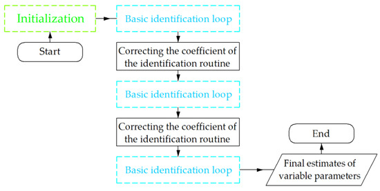
Figure 7.
Three-stage identification algorithm flow chart.
Table 2.
The boundaries, accuracy, and initial approximation of the identified parameters.
It should be noted that the DE created an initial population according to the normal distribution in the range represented in Table 2 where the number of individuals was equal to the number of initial parameters. The initial population was the same for both DE and DE-3.
The DE algorithm supposes the generation of random numbers. Therefore, to estimate the results’ repeatability, the identification was performed six times. Table 3 shows the results for six consecutive runs of the DE and DE-3. At the same time, the NM and NM-3 were started only once, because random number generation is not supposed in these algorithms.
Table 3.
Final values of the objective function/number of iterations for different algorithms.
Based on Table 3, it can be concluded that the NM algorithm provides the final value of the objective function 3.28/0.0095 = 345 times fewer than DE. In addition, NM demands the number of iterations 5383/2661 ≈ 2 times fewer than the DE. The NM-3 algorithm provides the final value of the objective function 0.379/0.0016 = 237 times fewer than DE-3. In addition, NM-3 demands the number of iterations 3332/1200 ≈ 3 times fewer than the DE-3. Table 4 represents the LSPMSM parameters’ values determined by the considered algorithms and real parameters. The best result out of six performed repetitions for the DE and DE-3 is shown in Table 4.
Table 4.
Identification results obtained by the considered algorithms and real motor parameters.
Figure 8 shows the objective function values for the considered optimization algorithms with the number of objective function calls, starting from the 120th NM call (1st generation for DE). Table 5 shows the mean values and RMS deviation of identified parameters obtained using the DE and DE-3 algorithms.
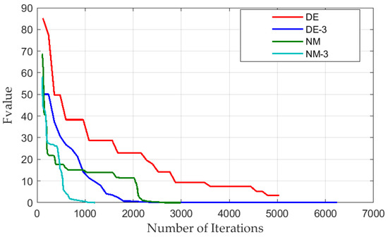
Figure 8.
The objective function values vs. the number of iterations for DE, DE-3, NM, and NM-3 algorithms.
Table 5.
Identification results obtained by the considered algorithms in comparison with real motor parameters.
The faster convergence of DE-3 compared to DE and NM-3 compared to NM confirms the effectiveness of the “stop and restart” technique used.
6. Identification with a Random Initial Approximation
The results of the considered identification algorithms were estimated at a random selection of the initial approximation. To perform that, the identification with six different random initial approximations was conducted. The random values were selected from the parameter ranges shown in Table 2.
Table 6 presents the results, such as the final values of the objective function and the number of iterations for the considered identification algorithms at six different initial approximations. Furthermore, Table 6 shows the mean and RMS deviations of the objective function values, calculated for six different initial approximations. Table 7 and Table 8 show the mean and RMS deviations of the parameters calculated by the considered algorithms. Figure 9 represents the dependencies of the objective function values on the number of objective function calls (iterations) for the best initial approximation.
Table 6.
The results of 6 executions for the considered identification algorithms with a random initial approximation: the objective function final values and the number of iterations.
Table 7.
Deviations of the LSPMSM parameters obtained using the NM identification algorithm with a random initial approximation.
Table 8.
Deviations of the LSPMSM parameters obtained using the DE identification algorithm with a random initial approximation.
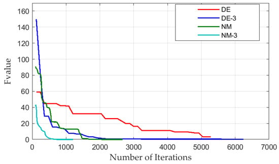
Figure 9.
The best objective function values vs. iterations for the random initial approximations.
With a fortunate choice of the initial approximation, when using the NM and NM-3 algorithms, the final value of the objective function deviated from the minimum value by a negligibly small amount (as a result of the identification, the objective function was reduced by four or more orders of magnitude). Using NM-3 required 2–3 times fewer function calls than NM (see Figure 7, Table 6).
With successful parametric identification, the objective function was reduced by about an order of magnitude when using DE and by two orders of magnitude when using DE-3. In addition, DE-3 required about two times fewer function calls than DE.
Although NM is a local search algorithm, and DE is a global one, in both cases, being stuck in a local minimum was possible (for example, see NM-3, start 1 and DE-3 start 6 in Table 6). Further, DE and DE-3 required more objective function calls compared to NM and NM-3.
From the above, we can conclude that in the considered application the Nelder–Mead method provides significant advantages over differential evolution. Therefore, it is preferable to run NM multiple times to find the best initial approximation rather than using DE. This does not preclude the use of DE to automatically find an initial approximation for NM.
The faster convergence of DE-3 compared to DE and NM-3 compared to NM confirms the effectiveness of the “stop and restart” technique used in the case of a random initial approximation, as well. Furthermore, even though NM is an unrestricted method, the results of identification using NM and NM-3 satisfy the conditions that all identified parameters (Ld, Lq, Ldσ; Lqσ; r′d; r′q, λ’0; J) are greater than zero; Ld > Lq; Ld >> Ldσ; Lq >> Lqσ, which confirms the ability of NM to successfully solve the problem under consideration.
7. Conclusions
The study is devoted to the comparative analysis of various computer-aided iterative identification methods based on optimization algorithms such as the differential evolution (DE) and the Nelder–Mead (NM) in LSPMSM lumped-parameter model identification. The comparison was carried out on the example of transients calculated for the LSPMSM model with given parameters.
Comparing the DE and NM algorithms at the same initial approximation, it can be concluded that the NM algorithm provided the final value of the objective function, proportional to the deviation of the identified parameters, 345 times fewer than DE. In addition, NM demanded the number of iterations to be two times fewer than DE. Comparing the DE and NM algorithms with a random initial approximation, it can be concluded that the NM provided the final value of the objective function 4.5·1010 times fewer than DE.
It can be concluded that, even though NM is an unrestricted local search method, it is able to successfully solve the problem under consideration, being more computationally efficient and accurate than DE. In this case, the DE method can be used at the initial stage of identification to find a suitable initial approximation for the NM. For a more accurate identification of the parameters, when a suitable initial approximation has already been found, the NM should be used.
In addition, in this study, it is proposed to stop and restart the considered identification procedures with a change in the algorithm parameters after a certain number of iterations and use the previously obtained results as a new initial approximation. Such multistage optimization (three stages have been found to be enough) leads to an increase in the computational speed and accuracy for both DE and NM. In this case, the NM algorithm provided the final value of the objective function 237 times fewer and required the number of iterations to be three times fewer than the DE with the same initial approximation. With a random initial approximation, in this case, the NM provided the final value of the objective function four times fewer than DE.
Although the article demonstrates the validity of the presented results only in the case of identifying the parameters of the LSPMSM model based on the results of simulated transients, in the future, the results will be used, and the conclusions will be verified when solving the problem of parametric identification of a real LSPMSM based on real transients.
Author Contributions
Conceptual approach, A.P., V.K. and V.P.; data curation, A.P. and S.O.; software, A.P., S.O. and V.K.; calculations and modelling, A.P., S.O., V.D., V.K. and V.P.; writing—original draft, A.P., S.O., V.D., V.K., V.G. and V.P.; visualization, A.P. and V.K.; review and editing, A.P., S.O., V.D., V.K., V.G. and V.P. All authors have read and agreed to the published version of the manuscript.
Funding
The work was partially supported by the Ministry of Science and Higher Education of the Russian Federation (through the basic part of the government mandate, Project No. FEUZ-2023-0013).
Institutional Review Board Statement
Not applicable.
Informed Consent Statement
Not applicable.
Data Availability Statement
Data are contained within the article.
Acknowledgments
The authors thank the editors and reviewers for their careful reading and constructive comments.
Conflicts of Interest
The authors declare no conflict of interest.
Glossary
| List of Abbreviations | |
| DE | Differential evolution |
| DE-3 | Differential evolution (three stages) |
| IM | Induction motor |
| LSPMSM | Line-start permanent magnet synchronous motor |
| NM | Nelder–Mead method |
| NM | Nelder–Mead method (three stages) |
| List of Mathematical Symbols | |
| f | Mains voltage frequency, Hz |
| F | Bearing friction and windage coefficient, N·m/(rad/s) |
| Fv | Parameter of differential evolution |
| Fvalue | Objective function value |
| iabc | Mains phase currents, A |
| Isd, Isq | Stator currents, A |
| I′rd, I′rq | Rotor currents, A |
| J | Moment of inertia of the motor, kg·m2 |
| kid, kiq, kω | Weight coefficients of the objective function |
| Lsd, Lsq | Stator total inductances, H |
| Lσd, Lσq | Rotor leakage inductances, H |
| qid,qiq, qω | Error terms in the objective function |
| r′d, r′q | Rotor resistances, Ohm |
| Rs | Stator resistance, Ohm |
| t | Time variable |
| T | Motor shaft torque, N·m |
| Tc | Constant component of the loading torque, N·m |
| Tload | Loading torque, N·m |
| Uabc | Mains phase voltage, V |
| Usd, Usq | Stator voltages along d and q axes, V |
| v | Mutated vector of differential evolution |
| v1, v2, v3 | Random vectors of differential evolution |
| x | Previous generation vector |
| Zp | Number of motor poles |
| α, β, γ, δ | Parameters of Nelder–Mead method |
| λ′rd, λ′rq | Rotor flux linkages, Wb |
| λsd, λsq | Stator flux linkages, Wb |
| λ′0 | Permanent magnet flux linkage, Wb |
| φ | Mechanical rotational angle, rad |
| ω | Angular frequency of the rotation of the motor shaft, rad/s |
References
- Kurihara, K.; Rahman, M. High-Efficiency Line-Start Interior Permanent-Magnet Synchronous Motors. IEEE Trans. Ind. Appl. 2004, 40, 789–796. [Google Scholar] [CrossRef]
- Kazakbaev, V.; Paramonov, A.; Dmitrievskii, V.; Prakht, V.; Goman, V. Indirect Efficiency Measurement Method for Line-Start Permanent Magnet Synchronous Motors. Mathematics 2022, 10, 1056. [Google Scholar] [CrossRef]
- Addendum to the Operating Instructions: AC Motors DR.71.J-DR.100.J with LSPM Technology, 21281793/EN, 09/2014, SEW Eurodrive. Available online: https://download.sew-eurodrive.com/download/pdf/21343799.pdf (accessed on 19 December 2022).
- de Almeida, A.T.; Ferreira, F.J.T.E.; Baoming, G. Beyond Induction Motors—Technology Trends to Move Up Efficiency. IEEE Trans. Ind. Appl. 2014, 50, 2103–2114. [Google Scholar] [CrossRef]
- Catalogue of Super Premium Efficiency SynchroVERT LSPM Motors. Available online: https://www.bharatbijlee.com/media/14228/synchrovert_catalogue.pdf (accessed on 19 December 2022).
- WQuattro, Super Premium Efficiency Motor, Product Catalogue, WEG Group—Motors Business Unit, Cod: 50025713, Rev: 03, Date (m/y): 07/2017. Available online: https://static.weg.net/medias/downloadcenter/h01/hfc/WEG-w22-quattro-european-market-50025713-brochure-english-web.pdf (accessed on 19 December 2022).
- KT-420-5, Operation of Bitzer Reciprocating Compressors with External Frequency Inverters, Bitzer, 01. 2022. Available online: https://www.bitzer.de/shared_media/html/kt-420/Resources/pdf/279303819.pdf (accessed on 19 December 2022).
- Do, N.; Le, T.; Ngo, X. Effect of Permanent Magnet Structure on The Performance of LSPMSM with a Power of 22 kW and 3000 rpm. IOP Conf. Ser. Earth Environ. Sci. 2022, 1111, 012047. [Google Scholar] [CrossRef]
- Zhao, W.; Tian, M.; Wang, X.; Sun, Y. Analysis of the Synchronization Process and the Synchronization Capability for a Novel 6/8-Pole Changing LSPMSM. IEEE Trans. Magn. 2020, 56, 1–6. [Google Scholar] [CrossRef]
- Melfi, M.J.; Umans, S.D.; Atem, J.E. Viability of Highly Efficient Multi-Horsepower Line-Start Permanent-Magnet Motors. IEEE Trans. Ind. Appl. 2015, 51, 120–128. [Google Scholar] [CrossRef]
- Isfahani, A.H.; Vaez-Zadeh, S.; Rahman, M.A. Evaluation of synchronization capability in line start permanent magnet synchronous motors. In Proceedings of the 2011 IEEE International Electric Machines & Drives Conference (IEMDC), Niagara Falls, ON, Canada, 15–18 May 2011; pp. 1346–1350. [Google Scholar] [CrossRef]
- Dinh, B.M. Optimal Rotor Design of Line Start Permanent Magnet Synchronous Motor by Genetic Algorithm. Adv. Sci. Technol. Eng. Syst. J. 2017, 2, 1181–1187. [Google Scholar] [CrossRef]
- Yan, B.; Yang, Y.; Wang, X. Design of a Large Capacity Line-Start Permanent Magnet Synchronous Motor Equipped With Hybrid Salient Rotor. IEEE Trans. Ind. Electron. 2020, 68, 6662–6671. [Google Scholar] [CrossRef]
- Palangar, M.F.; Mahmoudi, A.; Kahourzade, S.; Soong, W.L. Simultaneous Efficiency and Starting Torque Optimization of a Line-Start Permanent-Magnet Synchronous Motor Using Two Different Optimization Approaches. Arab. J. Sci. Eng. 2021, 46, 9953–9964. [Google Scholar] [CrossRef]
- Ferreira, F.; de Almeida, A.; Cistelecan, M. Voltage Unbalance Impact on the Performance of Line-Start Permanent-Magnet Synchronous Motors. In Proceedings of the 6th International Conference EEMODS, Nantes, France, 14–17 September 2009; pp. 123–137. [Google Scholar]
- Gnaciński, P.; Muc, A.; Pepliński, M. Influence of voltage subharmonics on line start permanent magnet synchronous motor. IEEE Access 2021, 9, 164275–164281. [Google Scholar] [CrossRef]
- Farooq, H.; Bracikowski, N.; La Delfa, P.; Hecquet, M. Estimation of Steady-State Torque of Line Start Permanent Magnet Synchronous Motor Using Reluctance Network Approach. In Proceedings of the International Conference of the IMACS TC1 Committee, Nancy, France, 17–20 May 2021; pp. 603–616. [Google Scholar] [CrossRef]
- RMahmoudi, A.; Roshandel, E.; Kahourzade, S.; Vakilipoor, F.; Drake, S. Bond graph model of line-start permanent-magnet synchronous motors. Electr. Eng. 2022, 1, 1–15. [Google Scholar] [CrossRef]
- Zohra, B.; Akar, M. Design Trends for Line Start Permanent Magnet Synchronous Motors. In Proceedings of the 3rd International Symposium on Multidisciplinary Studies and Innovative Technologies, ISMSIT, Ankara, Turkey, 11–13 October 2019. [Google Scholar] [CrossRef]
- Eker, M.; Zöhra, B.; Akar, M. Experimental performance verification of radial and axial flux line start permanent magnet synchronous motors. Elect. Eng. 2023, 1, 1–12. [Google Scholar] [CrossRef]
- Song, H.; Wang, R.; An, A.; Qiu, H. Influence of rotor magnetic circuit structure on eddy current loss of high voltage line-start permanent magnet synchronous motor. Int. Trans. Electr. Energy Syst. 2021, 31, 1–10. [Google Scholar] [CrossRef]
- Paramonov, A.; Oshurbekov, S.; Kazakbaev, V.; Prakht, V.; Dmitrievskii, V. Study of the Effect of Throttling on the Success of Starting a Line-Start Permanent Magnet Motor Driving a Centrifugal Fan. Mathematics 2022, 10, 4324. [Google Scholar] [CrossRef]
- Wang, D.; Wang, X.; Chen, H.; Zhang, R. Matlab/Simulink-Based Simulation of Line-start PMSM Used in Pump Jacks. In Proceedings of the 2nd IEEE Conference on Industrial Electronics and Applications, Harbin, China, 23–25 May 2007; pp. 1179–1181. [Google Scholar] [CrossRef]
- Paramonov, A.; Oshurbekov, S.; Kazakbaev, V.; Prakht, V.; Dmitrievskii, V. Investigation of the Effect of the Voltage Drop and Cable Length on the Success of Starting the Line-Start Permanent Magnet Motor in the Drive of a Centrifugal Pump Unit. Mathematics 2023, 11, 646. [Google Scholar] [CrossRef]
- Maraaba, L.S.; Al-Hamouz, Z.M.; Milhem, A.S.; Twaha, S. Comprehensive Parameters Identification and Dynamic Model Validation of Interior-Mount Line-Start Permanent Magnet Synchronous Motors. Machines 2019, 7, 4. [Google Scholar] [CrossRef]
- Dmitrievskii, V.; Prakht, V.; Kazakbaev, V.; Oshurbekov, S.; Sokolov, I. Developing ultra premium efficiency (IE5 class) magnet-free synchronous reluctance motor. In Proceedings of the 6th International Electric Drives Production Conference (EDPC), Nuremberg, Germany, 30 November–1 December 2016; pp. 2–7. [Google Scholar] [CrossRef]
- Zhan, X.; Zeng, G.; Liu, J.; Wang, Q.; Ou, S. A Review on Parameters Identification Methods for Asynchronous Motor. Int. J. Adv. Comput. Sci. Appl. 2015, 6. [Google Scholar] [CrossRef]
- Deng, A.; Zou, J.; Shao, Z.; Huang, G.; Shi, L.; Deng, W.; Antong, D. Improvement on asynchronous motor system identification based on interactive MRAS. In Proceedings of the 27th Chinese Control and Decision Conference (CCDC), Qingdao, China, 23–25 May 2015; pp. 448–453. [Google Scholar] [CrossRef]
- Balara, D.; Timko, J.; Zilkova, J.; Lešo, M. Neural networks application for mechanical parameters identification of asynchronous motor. Neural Netw. World 2017, 27, 259–270. [Google Scholar] [CrossRef]
- Kryukov, A.; Suslov, K.; Ilyushin, P.; Akhmetshin, A. Parameter Identification of Asynchronous Load Nodes. Energies 2023, 16, 1893. [Google Scholar] [CrossRef]
- Yang, T.-G.; Gui, W.-H. Stator resistance identification for induction motor based on particle swarm optimization neural network observer. Dianji Yu Kongzhi Xuebao/Electr. Mach. Control. 2015, 19, 89–95. [Google Scholar] [CrossRef]
- Wang, L.; Liu, Y. Application of Simulated Annealing Particle Swarm Optimization Based on Correlation in Parameter Identification of Induction Motor. Math. Probl. Eng. 2018, 2018, 1869232. [Google Scholar] [CrossRef]
- Guangyi, C.; Wei, G.; Kaisheng, H. On Line Parameter Identification of an Induction Motor Using Improved Particle Swarm Optimization. In Proceedings of the 26th Chinese Control Conference, CCC, Zhangjiajie, China, 26–31 July 2007; pp. 745–749. [Google Scholar] [CrossRef]
- Marčič, T.; Štumberger, B.; Štumberger, G. Differential-Evolution-Based Parameter Identification of a Line-Start IPM Synchronous Motor. IEEE Trans. Ind. Electron. 2014, 61, 5921–5929. [Google Scholar] [CrossRef]
- Su, G.; Wang, P.; Guo, Y.; Cheng, G.; Wang, S.; Zhao, D. Multiparameter Identification of Permanent Magnet Synchronous Motor Based on Model Reference Adaptive System—Simulated Annealing Particle Swarm Optimization Algorithm. Electronics 2022, 11, 159. [Google Scholar] [CrossRef]
- Kaššay, P.; Grega, R. Measuring Mass Moment of Inertia of a Rotor—Two Simple Methods Using No Special Equipment. In Current Methods of Construction Design: Proceedings of the ICMD 2018; Springer International Publishing: Basel, Switzerland, 2020; pp. 303–315. [Google Scholar] [CrossRef]
- Markus Buehren. Differential Evolution. MATLAB Central File Exchange. 2023. Available online: https://www.mathworks.com/matlabcentral/fileexchange/18593-differential-evolution (accessed on 3 March 2023).
- Price, K.; Storn, R.; Lampinen, J. Differential Evolution: A Practical Approach to Global Optimization; Springer: Berlin/Heidelberg, Germany, 2005. [Google Scholar]
- Fminsearch. MathWorks. Available online: https://www.mathworks.com/help/matlab/ref/fminsearch.html (accessed on 20 June 2023).
- Nelder, J.; Mead, R. A Simplex Method for Function Minimization. Comput. J. 1965, 7, 308–313. [Google Scholar] [CrossRef]
- Wang, H.; Ge, X.; Liu, Y.-C. Second-Order Sliding-Mode MRAS Observer-Based Sensorless Vector Control of Linear Induction Motor Drives for Medium-Low Speed Maglev Applications. IEEE Trans. Ind. Electron. 2018, 65, 9938–9952. [Google Scholar] [CrossRef]
- Simulate Simulink Model. MATLAB Documentation. © 1994–2023 The MathWorks, Inc. Available online: https://www.mathworks.com/help/simulink/slref/sim.html (accessed on 20 June 2023).


Disclaimer/Publisher’s Note: The statements, opinions and data contained in all publications are solely those of the individual author(s) and contributor(s) and not of MDPI and/or the editor(s). MDPI and/or the editor(s) disclaim responsibility for any injury to people or property resulting from any ideas, methods, instructions or products referred to in the content. |
© 2023 by the authors. Licensee MDPI, Basel, Switzerland. This article is an open access article distributed under the terms and conditions of the Creative Commons Attribution (CC BY) license (https://creativecommons.org/licenses/by/4.0/).