

Fault Diagnosis of Wind Turbine with Alarms Based on Word Embedding and Siamese Convolutional Neural Network


Abstract
Featured Application
Abstract
1. Introduction
- The unlabeled and labeled alarms can be collaboratively applied in the proposed S-ECNN model, which can effectively improve the fault diagnosis accuracy of wind turbines.
- The potential relationships among individual alarms are captured in n-dimensional space using a word embedding method, which considers not only the alarm order but also the frequency of occurrence.
2. Background
2.1. Wind Turbine Alarms
2.2. Maintenance Records
- When a wind turbine is shut down due to alarms, manual maintenance will be performed. However, many alarms cannot cause a shutdown. Thus, the fault events that trigger these alarms are not available.
- Some alarms that can cause a shutdown are eliminated by the self-inspection function and thus have no recorded fault events.
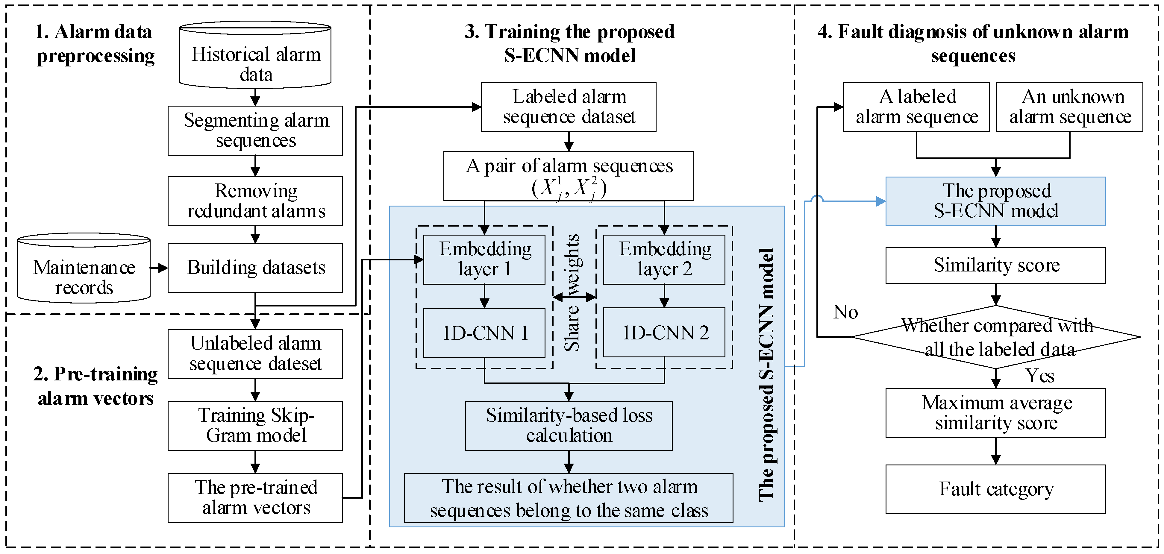
3. The Proposed Fault Diagnosis Methodology
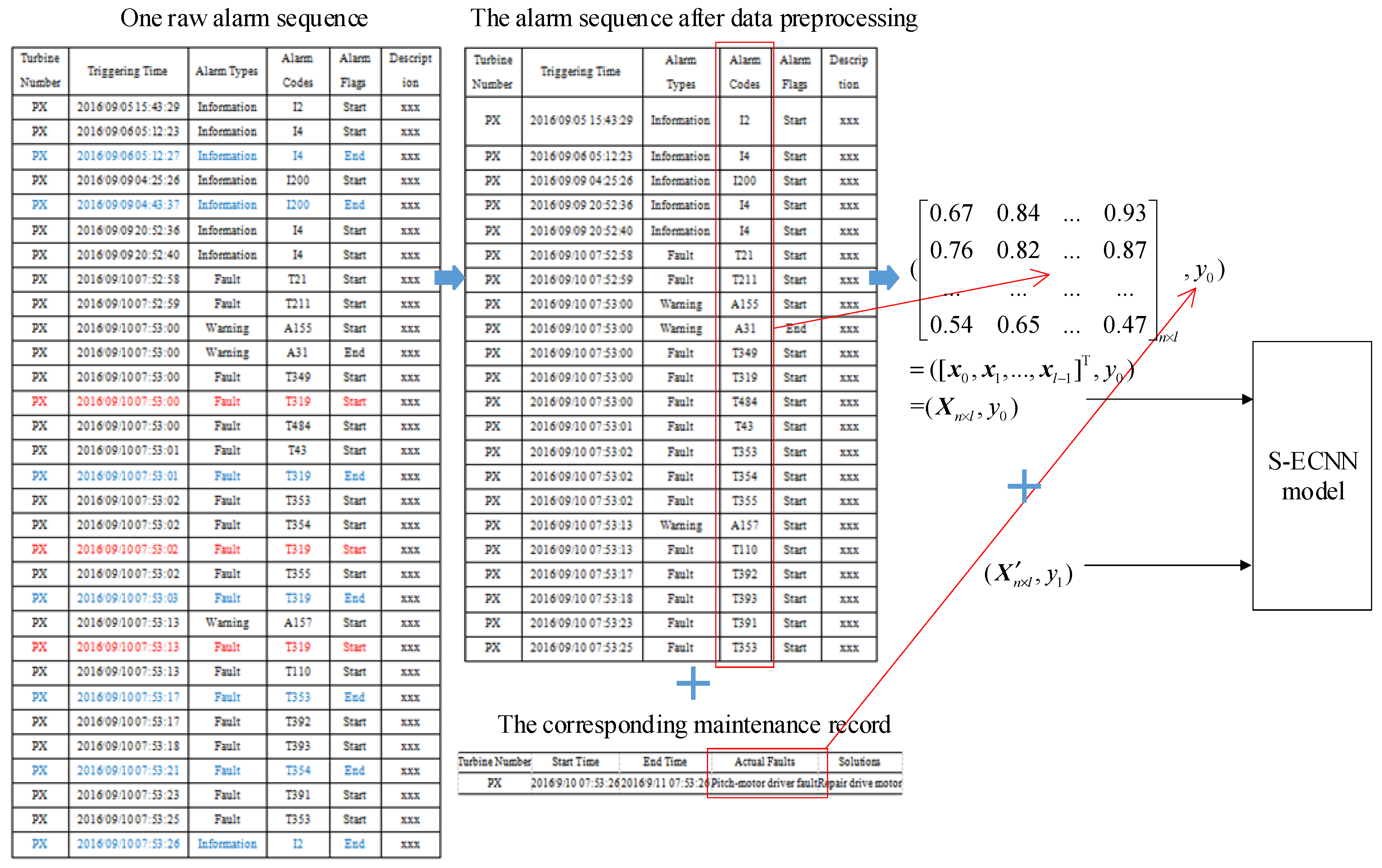
3.1. Alarm Data Preprocessing
3.1.1. Segmenting Alarm Sequences
3.1.2. Removing Redundant Alarms
3.1.3. Building Dataset
3.2. Pretraining Alarm Vectors
3.3. The Proposed S-ECNN Model
3.3.1. The Embedding Layer
3.3.2. 1D-CNN
3.3.3. Distance Layer and Output Layer
3.4. Fault Diagnosis of Unknown Alarm Sequences
4. Results and Discussion
4.1. Data Description
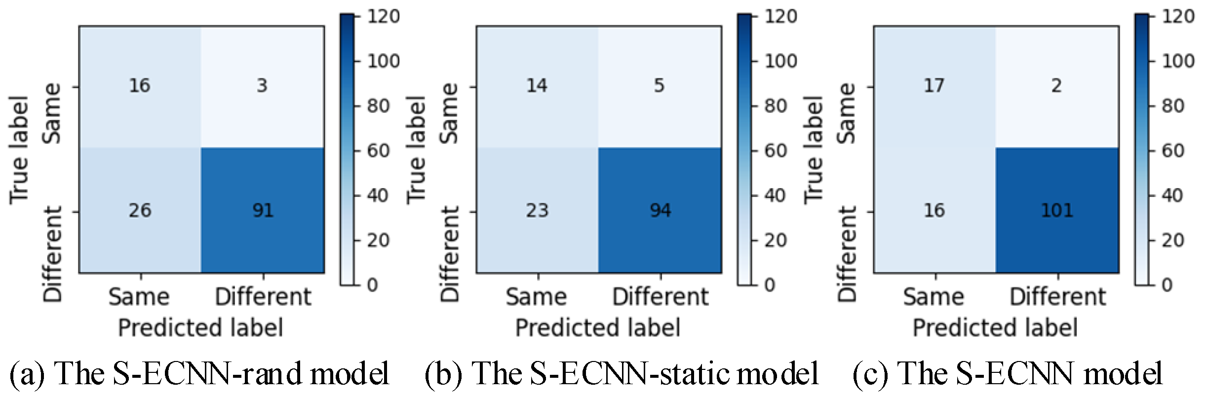
4.2. Model Variants
4.3. Evaluation of Pretrained Alarm Vectors
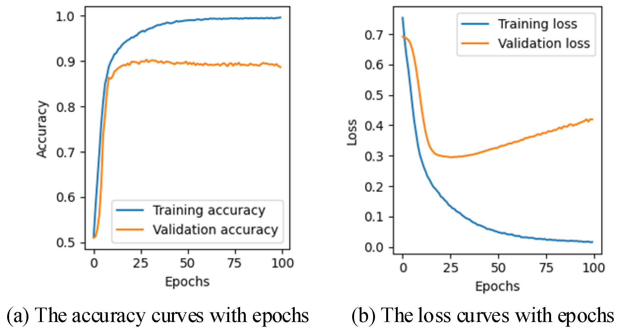
4.4. Evaluation of Experimental Results
4.4.1. Evaluation of Distinguishing Ability
4.4.2. Evaluation of Fault Diagnosis Method
5. Conclusions
Author Contributions
Funding
Institutional Review Board Statement
Informed Consent Statement
Data Availability Statement
Conflicts of Interest
References
- Lee, J.; Zhao, F. Global Wind Report 2022; Global Wind Energy Council: Brussels, Belgium, 2022; 158p, Available online: https://gwec.net/global-wind-report–2022/ (accessed on 4 April 2022).
- Ren, G.; Liu, J.; Wan, J.; Guo, Y.D.; Yu, D. Overview of wind power intermittency: Impacts, measurements, and mitigation solutions. Appl. Energy 2017, 204, 47–65. [Google Scholar] [CrossRef]
- Spinato, F.; Tavner, P.J.; Bussel, G.L.; Koutoulakos, E. Reliability of wind turbine subassemblies. IET Renew. Power Gener. 2009, 3, 387–401. [Google Scholar] [CrossRef]
- Yang, W.; Tavner, P.J.; Crabtree, C.J.; Feng, Y.; Qiu, Y. Wind turbine condition monitoring: Technical and commercial challenges. Wind Energy 2014, 17, 673–693. [Google Scholar] [CrossRef]
- Martin, R.; Lazakis, I.; Barbouchi, S.; Johanning, L. Sensitivity analysis of offshore wind farm operation and maintenance cost and availability. Renew. Energy 2016, 85, 1226–1236. [Google Scholar] [CrossRef]
- Helbing, G.; Ritter, M. Deep Learning for fault detection in wind turbines. Renew. Sustain. Energy Rev. 2018, 98, 189–198. [Google Scholar] [CrossRef]
- Peeters, C.; Guillaume, P.; Helsen, J. Vibration-based bearing fault detection for operations and maintenance cost reduction in wind energy. Renew. Energy 2018, 116, 74–87. [Google Scholar] [CrossRef]
- Zhang, L.; Zhang, H.; Cai, G. The multiclass fault diagnosis of wind turbine bearing based on multisource signal fusion and deep learning generative model. IEEE Trans. Instrum. Meas. 2022, 71, 3514212. [Google Scholar] [CrossRef]
- Tiboni, M.; Remino, C.; Bussola, R.; Amici, C. A review on vibration-based condition monitoring of rotating machinery. Appl. Sci. 2022, 12, 972. [Google Scholar] [CrossRef]
- Coronado, D.; Wenske, J. Monitoring the oil of wind-turbine gearboxes: Main degradation indicators and detection methods. Machines 2018, 6, 25. [Google Scholar] [CrossRef]
- Shahriar, M.R.; Borghesani, P.; Tan, A.C. Electrical signature analysis-based detection of external bearing faults in electromechanical drivetrains. IEEE Trans. Industr. Electron. 2018, 65, 5941–5950. [Google Scholar] [CrossRef]
- Wei, L.; Qian, Z.; Zareipour, H. Wind turbine pitch system condition monitoring and fault detection based on optimized relevance vector machine regression. IEEE Trans. Sustain. Energy 2020, 11, 2326–2336. [Google Scholar] [CrossRef]
- Jin, X.; Xu, Z.; Qiao, W. Conditon monitoring of wind turbine generators using SCADA data analysis. IEEE Trans. Sustain. Energy 2021, 12, 202–210. [Google Scholar] [CrossRef]
- Wen, W.; Liu, Y.; Sun, R.; Liu, Y. Research on anomaly detection of wind farm SCADA wind speed data. Energies 2022, 15, 5869. [Google Scholar] [CrossRef]
- Qiu, Y.; Feng, Y.; Tavner, P.; Richardson, P.; Erdos, G.; Chen, B. Wind turbine SCADA alarm analysis for improving reliability. Wind Energy 2012, 15, 951–966. [Google Scholar] [CrossRef]
- Wang, J.; Yang, F.; Chen, T.; Shah, S.L. An overview of industrial alarm systems: Main causes for alarm overloading, research status, and open problems. IEEE Trans. Autom. Sci. Eng. 2016, 13, 1045–1061. [Google Scholar] [CrossRef]
- Qiao, W.; Lu, D. A survey on wind turbine condition monitoring and fault diagnosis—Part I: Components and subsystems. IEEE Trans. Ind. Electron. 2015, 62, 6536–6545. [Google Scholar] [CrossRef]
- Wang, J.; Li, H.; Huang, J.; Su, C. A data similarity based analysis to consequential alarms of industrial processes. J. Loss Prev. Process Ind. 2015, 35, 29–34. [Google Scholar] [CrossRef]
- Rodríguez-López, M.A.; López-González, L.M.; López-Ochoa, L.M. Development of indicators for the detection of equipment malfunctions and degradation estimation based on digital signals (alarms and events) from operation SCADA. Renew. Energy 2022, 18, 288–296. [Google Scholar] [CrossRef]
- Chen, B.; Qiu, Y.N.; Feng, Y.; Tavner, P.J.; Song, W.W. Wind turbine SCADA alarm pattern recognition. In Proceedings of the IET Conference on Renewable Power Generation, Edinburgh, UK, 5–8 September 2011. [Google Scholar]
- Tong, C.; Guo, P. Data mining with improved Apriori algorithm on wind generator alarm data. In Proceedings of the 25th Chinese Control and Decision Conference, Guiyang, China, 25–27 May 2013. [Google Scholar]
- Leahy, K.; Gallagher, C.; O’Donovan, P.; O’Sullivan, D.T. Cluster analysis of wind turbine alarms for characterising and classifying stoppages. IET Renew. Power Gener. 2018, 12, 1146–1154. [Google Scholar] [CrossRef]
- Qiu, Y.; Feng, Y.; Infield, D. Fault diagnosis of wind turbine with SCADA alarms based multidimensional information processing method. Renew. Energy 2020, 145, 1923–1931. [Google Scholar] [CrossRef]
- Wei, L.; Qian, Z.; Pei, Y.; Wang, J. Wind turbine fault diagnosis by the approach of SCADA alarms analysis. Appl. Sci. 2022, 12, 69. [Google Scholar] [CrossRef]
- 20/30400796 DC; Management of Alarms Systems for the Process Industries. International Society of Automation: Miami, FL, USA, 2020.
- Zhang, C.; Guo, R.; Ma, X.; Kuai, X.; He, B. W-TextCNN: A TextCNN model with weighted word embeddings for Chinese address pattern classification. Comput. Environ. Urban Syst. 2022, 95, 101819. [Google Scholar] [CrossRef]
- Naili, M.; Chaibi, A.H.; Ghezala, H.H.B. Comparative study of word embedding methods in topic segmentation. Proc. Comput. Sci. 2017, 112, 340–349. [Google Scholar] [CrossRef]
- Mikolov, T.; Sutskever, I.; Chen, K.; Corrado, G.; Dean, J. Distributed Representations of Words and Phrases and Their. Compositionality. Patent 10.48550/arXiv.1310.4546, 16 October 2013. Available online: https://arxiv.org/pdf/1310.4546.pdf (accessed on 16 October 2013).
- Cai, S.; Palazoglu, A.; Zhang, L.; Hu, J. Process alarm prediction using deep learning and word embedding methods. ISA Trans. 2019, 85, 274–283. [Google Scholar] [CrossRef] [PubMed]
- Bromley, J.; Guyon, I.; LeCun, Y.; Säckinger, E.; Shah, R. Signature verification using a “siamese” time delay neural network. Int. J. Pattern Recognit. Artif. Intell. 1993, 7, 669–688. [Google Scholar] [CrossRef]
- Huang, L.; Chen, Y. Dual-path siamese CNN for hyperspectral image classification with limited training samples. IEEE Geosci. Remote Sens. Lett. 2021, 18, 518–522. [Google Scholar] [CrossRef]
- Bharadwaj, S.; Prasad, S.; Almekkawy, M. An upgraded siamese neural network for motion tracking in ultrasound image sequences. IEEE Trans. Ultrason. Ferroelectr. Freq. Control 2021, 68, 3515–3527. [Google Scholar] [CrossRef]
- Zhou, X.; Liang, W.; Shimizu, S.; Ma, J.; Jin, Q. Siamese neural network based few-shot learning for anomaly detection in industrial cyber-physical systems. IEEE Trans. Ind. Inform. 2021, 17, 5790–5798. [Google Scholar] [CrossRef]
- Zhu, J.; Jang-Jaccard, J.; Watters, P.A. Multi-loss siamese neural network with batch normalization layer for malware detection. IEEE Access 2020, 8, 171542–171550. [Google Scholar] [CrossRef]
- Witten, I.H.; Frank, E.; Hall, M.A. Credibility: Evaluating what’s been learned. In Data Mining: Practical Machine Learning Tools and Techniques, 3rd ed.; Morgan Kaufmann: Burlington, MA, USA, 2011; pp. 147–187. [Google Scholar]
- Pezzotti, N.; Thijssen, J.; Mordvintsev, A.; Hollt, T.; Van Lew, B.; Lelieveldt, B.P.; Eisemann, E.; Vilanova, A. GPGPU linear complexity t-SNE optimization. IEEE Trans. Vis. Comput. Graph. 2020, 26, 1172–1181. [Google Scholar] [CrossRef]
- Geibel, M.; Bangga, G. Data reduction and reconstruction of wind turbine wake employing data driven approaches. Energies 2022, 15, 3773. [Google Scholar] [CrossRef]


| Turbine Number | Triggering Time | Alarm Types | Alarm Codes | Alarm Flags | Description |
|---|---|---|---|---|---|
| P01 | 2017/5/22 16:30:05 | Information | I2 | Start | The wind turbine is started |
| P01 | 2017/5/22 17:38:18 | Warning | A264 | Start | The first measuring point temperature of generator stator is high |
| P01 | 2017/5/22 17:38:37 | Warning | A264 | End | The first measuring point temperature of generator stator is high |
| P01 | 2017/5/22 17:38:51 | Fault | T21 | Start | The communication of the pitch system is an error |
| P01 | 2017/5/22 17:38:52 | Information | I2 | End | The wind turbine is started |
| P01 | 2017/5/23 00:15:20 | Fault | T21 | End | The communication of the pitch system is an error |
| Turbine Number | Start Time | End Time | Actual Faults | Solutions |
|---|---|---|---|---|
| P01 | 2016/12/21 17:34:00 | 2016/12/25 12:45:00 | A slip ring is damaged | Replace the slip ring |
| Layers | Filters | Stride | Output Size | Layers |
|---|---|---|---|---|
| Convolutional-ReLU | 128 filters size of 3 × 100 | 1 | 128 × 30 × 1 | Convolutional-ReLU |
| Max-Pooling | 3 | 3 | 128 × 10 × 1 | Max-Pooling |
| Convolutional-ReLU | 32 filters size of 3 | 1 | 32 × 10 × 1 | Convolutional-ReLU |
| Max-Pooling | 3 | 3 | 32 × 4 × 1 | Max-Pooling |
| Flatten layer | - | - | 128 × 1 | Flatten layer |
| Label | Fault Categories | Number of Alarm Sequences (Training Set/Test Set) |
|---|---|---|
| F1 | Hub speed encoder fault | 8 (6/2) |
| F2 | Pitch system communication fault | 8 (6/2) |
| F3 | Vibration sensor fault | 9 (7/2) |
| F4 | Pitch motor driver fault | 10 (8/2) |
| F5 | Generator stator fault | 10 (8/2) |
| F6 | Frequency-converter communication fault | 14 (11/3) |
| F7 | Wind vane fault | 15 (11/4) |
| Model | Accuracy | Recall | Precision | Specificity | F1-Score |
|---|---|---|---|---|---|
| S-ECNN-rand | 78.7% | 84.2% | 38.1% | 77.8% | 52.5% |
| S-ECNN-static | 79.4% | 73.7% | 37.8% | 80.3% | 50.0% |
| S-ECNN | 86.8% | 89.5% | 51.5% | 86.3% | 65.4% |
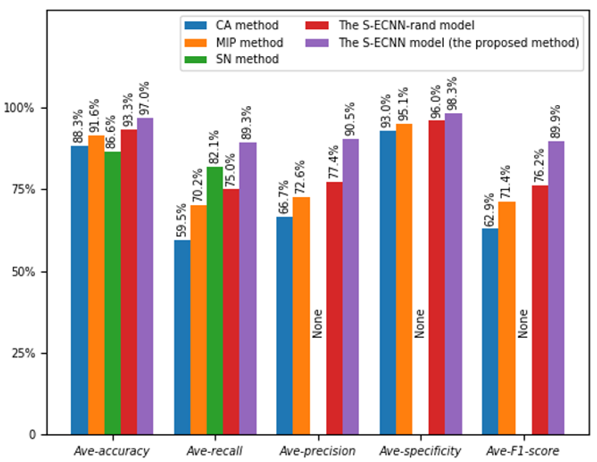
| Method | Ave-Accuracy | Ave-Recall | Ave-Precision | Ave-Specificity | Ave-F1_Score |
|---|---|---|---|---|---|
| S-ECNN-rand | 93.3% | 75.0% | 77.4% | 96.0% | 76.2% |
| S-ECNN-static | 91.6% | 73.8% | 76.2% | 95.2% | 75.0% |
| S-ECNN | 97.0% | 89.3% | 90.5% | 98.3% | 89.9% |
Disclaimer/Publisher’s Note: The statements, opinions and data contained in all publications are solely those of the individual author(s) and contributor(s) and not of MDPI and/or the editor(s). MDPI and/or the editor(s) disclaim responsibility for any injury to people or property resulting from any ideas, methods, instructions or products referred to in the content. |
© 2023 by the authors. Licensee MDPI, Basel, Switzerland. This article is an open access article distributed under the terms and conditions of the Creative Commons Attribution (CC BY) license (https://creativecommons.org/licenses/by/4.0/).
Share and Cite
Wei, L.; Qu, J.; Wang, L.; Liu, F.; Qian, Z.; Zareipour, H. Fault Diagnosis of Wind Turbine with Alarms Based on Word Embedding and Siamese Convolutional Neural Network. Appl. Sci. 2023, 13, 7580. https://doi.org/10.3390/app13137580
Wei L, Qu J, Wang L, Liu F, Qian Z, Zareipour H. Fault Diagnosis of Wind Turbine with Alarms Based on Word Embedding and Siamese Convolutional Neural Network. Applied Sciences. 2023; 13(13):7580. https://doi.org/10.3390/app13137580
Chicago/Turabian StyleWei, Lu, Jiaqi Qu, Liliang Wang, Feng Liu, Zheng Qian, and Hamidreza Zareipour. 2023. "Fault Diagnosis of Wind Turbine with Alarms Based on Word Embedding and Siamese Convolutional Neural Network" Applied Sciences 13, no. 13: 7580. https://doi.org/10.3390/app13137580
APA StyleWei, L., Qu, J., Wang, L., Liu, F., Qian, Z., & Zareipour, H. (2023). Fault Diagnosis of Wind Turbine with Alarms Based on Word Embedding and Siamese Convolutional Neural Network. Applied Sciences, 13(13), 7580. https://doi.org/10.3390/app13137580