A Harmonic and Interharmonic Detection Method for Power Systems Based on Enhanced SVD and the Prony Algorithm

Abstract

To address the problem of harmonic pollution in power systems, a harmonic and interharmonic detection method based on the adaptive order and the dominant factor algorithms is proposed. The proposed method greatly improves the accuracy and precision of harmonic detection, overcoming the notorious problem of high sensitivity to noise of the traditional Prony algorithm that often leads to unsatisfactory detection results. In the proposed method, the “adaptive order determination” algorithm is first used to determine the optimal order of Singular Value Decomposition (SVD) denoising, resulting in a more accurate distinction between signal and noise components. Then, signal reconstruction is carried out to effectively remove noise components to enhance the denoising ability of SVD. This mitigates the Prony algorithm’s high sensitivity to noise and greatly reduces the amplitude of false components in the fitting results. Finally, the dominant factor algorithm is applied to accurately screen out the non-false components in Prony’s fitting results. Simulation results show that the proposed method can effectively reduce signal noise in different noise environments with noise intensities ranging from 5 dB to 30 dB, achieving an average signal-to-noise ratio improvement of around 20 dB. Meanwhile, the identification and screening results of harmonic and interharmonic components in the signal are accurate and reliable, with detection errors in amplitude, frequency, and phase at around 0.5%, 0.01%, and 0.5%, respectively. Overall, the proposed method is well suited for detecting harmonics and interharmonics in power systems under various noise environments.

1. Introduction

With the emergence of the grid connection of new energy sources and the increasing use of nonlinear electrical equipment, harmonic pollution in power systems has become more and more severe, posing a threat to power quality, power supply safety, and economic benefit. Therefore, there has been growing demand to curb harmonic pollution to ensure power quality. In this context, accurate detection of harmonics and interharmonics in signals is a prerequisite for effective harmonic pollution management [1,2,3,4].

At present, the detection of harmonics and interharmonics is mainly divided into frequency domain analysis and time-domain analysis. Frequency domain analysis mainly refers to Fourier transform, which is simple in method and fast in computation, but suffers from spectrum leakage and the fence effect [5,6,7]. Time-domain analysis includes Wave Transform (WT) [8,9,10], Empirical Mode Decomposition (EMD) [11,12,13], Hilbert–Huang Transform (HHT) [14,15,16,17,18], the Prony algorithm [19,20,21,22], etc. WT is, in essence, Fourier transform with an adjustable window size, which can reflect the entire process of signal changes. However, difficulties arise in selecting an appropriate wave basis function. When using WT, many tests must be carried out to determine the most suitable wave basis, which is not self-adaptive to the signal. EMD is an adaptive decomposition method for nonlinear and non-stationary time series data. However, mode aliasing exists in the decomposition process of EMD, which leads to different time-scale components appearing in the same characteristic mode function [23]. HHT is composed of EMD and Hilbert transform, which can be adaptively decomposed with high precision according to the signal. Nevertheless, it is susceptible to end effects and severe mode aliasing effects. Literature [24] uses a multi-resolution analysis of WT to process the original signal. Then, the EMD algorithm is used to obtain a series of Intrinsic Mode Function (IMF) components from the processed signals, and fundamental and harmonic components are extracted from the IMF components. Finally, the Hilbert transform is used to calculate the frequency and amplitude of the signal. The Prony algorithm uses a series of exponential formal functions to fit the sample signal, which can extract the frequency, amplitude, phase and attenuation factor of the signal. The frequency resolution is high and the calculation is simple. Nevertheless, the Prony algorithm is known to be highly sensitive to noise, and its fitting results often contain many false components and data screening in the fitting results. In literature [25], the Prony algorithm is used to screen the detection results of harmonics and eliminate false components. However, due to the absence of signal denoising, in the presence of strong environmental noise, the fitting accuracy would be reduced and the amplitude of false components in the fitting results can be higher than that of non-false components, which may lead to unsatisfactory screening results. Literature [26] improves the denoising of Variational Mode Decomposition (VMD) and combines the Prony-GSO algorithm to detect harmonics. Yet, a mode aliasing effect exists in the VMD method, and the signal is distorted to some extent after denoising, which affects the detection accuracy. Literature [27] adopts Singular Value Decomposition (SVD) to denoise signals and determine the denoising order by the rate of singular value change to improve SVD’s denoising capability and overcome the noise sensitivity of the Prony algorithm. Despite its effectiveness, the adaptability of this method is limited: in the presence of strong environment noise, the singular value does not change obviously and the denoising ability decreases.

In view of the advantages and disadvantages of the aforementioned methods, this paper proposes a novel harmonic and interharmonic detection method based on enhanced SVD and the Prony algorithm. The method first applies SVD to denoise signals and proposes an adaptive order determination method to select the optimal order for SVD denoising. This enhances the denoising capability and has strong adaptability to different noise environments, thereby overcoming the Prony algorithm’s sensitivity to noise. Next, the Prony algorithm is applied to detect the frequency, amplitude, phase and attenuation factor of harmonics and interharmonics in the denoised signal. Finally, the dominant factor algorithm is proposed to screen the non-false components in the results. Simulation results show that the proposed method possesses remarkable noise denoising capability and adaptability to different noise intensities. The Signal-to-Noise Ratio (SNR) of the signal can be increased by about 20 dB on average, which makes the false components in the fitting result of the Prony algorithm small in amplitude and fast in attenuation. Moreover, the dominant factor algorithm can quickly and accurately screen out the non-false components, and the detection accuracy of frequency, amplitude and phase is high, which verifies the effectiveness and accuracy of this method.

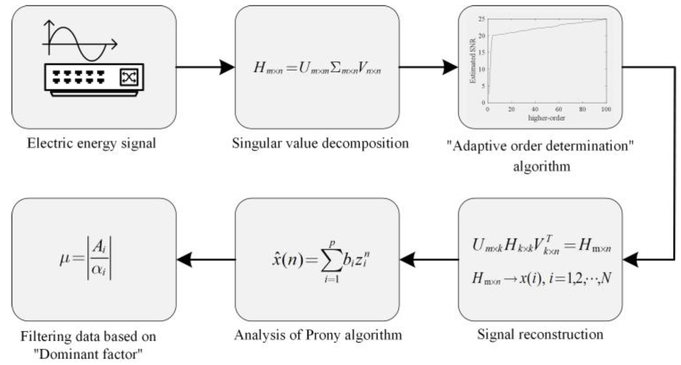
2. System Structure

The Prony algorithm is a mathematical model that employs a linear combination of exponential functions to fit the sample data. It has the characteristics of high-frequency resolution and high-frequency estimation accuracy. However, the Prony algorithm is very sensitive to noise, which leads to suboptimal detection accuracy. Moreover, there are many false components in the fitting results of the Prony algorithm, and the amplitude of false components is higher than that of non-false components, which interferes with data screening. In light of these drawbacks, this paper proposes a novel harmonic and interharmonic detection method based on enhanced SVD and the Prony algorithm, whose process is illustrated in Figure 1.

Targeting Prony algorithm’s sensitivity to noise, this method first applies the SVD denoising algorithm to denoise the matrix constructed by the electric energy signal. Since the choice of the characteristic matrix’s order in the SVD denoising process affects the signal denoising effect, the “adaptive order determination” algorithm is proposed to determine the optimal order of the characteristic matrix for enhanced denoising effect of SVD. The Prony algorithm is then carried out on the reconstructed one-dimensional electric energy signal after denoising and the fitting result of the signal is obtained. Finally, a method based on the dominant factor is used to filter the fitting results and find out the non-false components representing harmonic and interharmonic parameters. The non-false component is composed of amplitude, frequency and phase, which is the detection result of harmonic and interharmonic signal parameters in the signal.

3. Theoretical Analysis

In general, collected electric energy signals always contain noise components. The better these noise components can be filtered, the stronger the harmonics and interharmonics detection performance the subsequent Prony algorithm can deliver. The traditional SVD denoising method, when used for signal denoising, often suffers from poor adaptability to signals with different noise intensities, which may lead to insufficient or excessive filtering of noise components, damaging useful signals and resulting in poor denoising effect. Therefore, this paper proposes an improved method to enhance the denoising ability of SVD and overcome the drawbacks of traditional SVD denoising.

3.1. Singular Value Decomposition (SVD) Denoising

Consider a sampled electric energy signal $\mathrm{X}\left(i\right)=[x\left(1\right),x\left(2\right),\cdots ,x\left(N\right)]$, which can be written as

$$\mathrm{X}\left(i\right)=\mathrm{S}\left(i\right)+\mathrm{E}\left(i\right),i=\mathrm{1,2},\cdots ,\mathrm{N},$$

(1)

where $\mathrm{S}\left(i\right)$ denotes the noiseless signal and $\mathrm{E}\left(i\right)$ denotes the pure noise signal. SVD denoising aims to remove $\mathrm{E}\left(i\right)$ while retaining $\mathrm{S}\left(i\right)$.

$$\mathit{H}=\left[\begin{array}{ccc}\begin{array}{cc}x\left(1\right)& x\left(2\right)\\ x\left(2\right)& x\left(3\right)\end{array}& \cdots & \begin{array}{c}x\left(n\right)\\ x\left(n+1\right)\end{array}\\ \begin{array}{cc}⋮& ⋮\end{array}& \ddots & ⋮\\ \begin{array}{cc}x\left(m\right)& x\left(m+1\right)\end{array}& \cdots & x\left(\mathrm{N}\right)\end{array}\right],$$

(2)

where N is the length of the one-dimensional signal $\mathrm{X}\left(i\right)$ and m = N + 1 − n.

Hence, for the real matrix ${\mathit{H}}_{m\times n}\in R^{m\times m}$, there must be an orthogonal matrix ${\mathit{U}}_{m\times m}\in R^{m\times m}$ of order m and an orthogonal matrix ${\mathit{V}}_{n\times n}\in R^{n\times n}$ of order n which satisfy the following relationship:

$${\mathit{H}}_{m\times n}={\mathit{U}}_{m\times m}{\mathsf{\Sigma }}_{m\times n}{\mathit{V}}_{n\times n}^T,$$

(3)

where ${\mathsf{\Sigma }}_{m\times n}$ is a real diagonal matrix of $m\times n$: ${\mathsf{\Sigma }}_{m\times n}=\mathrm{d}\mathrm{i}\mathrm{a}\mathrm{g}\left({\lambda }_1,{\lambda }_2,\cdots ,{\lambda }_q\right)$ in which $q=\mathrm{m}\mathrm{i}\mathrm{n}(m,n)$ and ${\lambda }_q$ denotes all the non-zero singular values of matrix ${\mathit{H}}_{m\times n}$(${\lambda }_1\ge {\lambda }_2\ge \cdots \ge {\lambda }_q>0$). The first $k$ singular values represent the noiseless signal information in the ${\mathit{H}}_{m\times n}$ matrix, and the last $(q-k)$ singular values represent the noise information ($q>k>0)$.

The last $(q-k)$ singular values are set to zero, after which signal reconstruction is carried out to obtain the signal after denoising. Hence, the determination of effective order $k$ is crucial to the denoising effect of SVD. To this end, an “adaptive order determination” algorithm is proposed in this paper to deduce the optimal effective order for enhanced denoising performance of SVD.

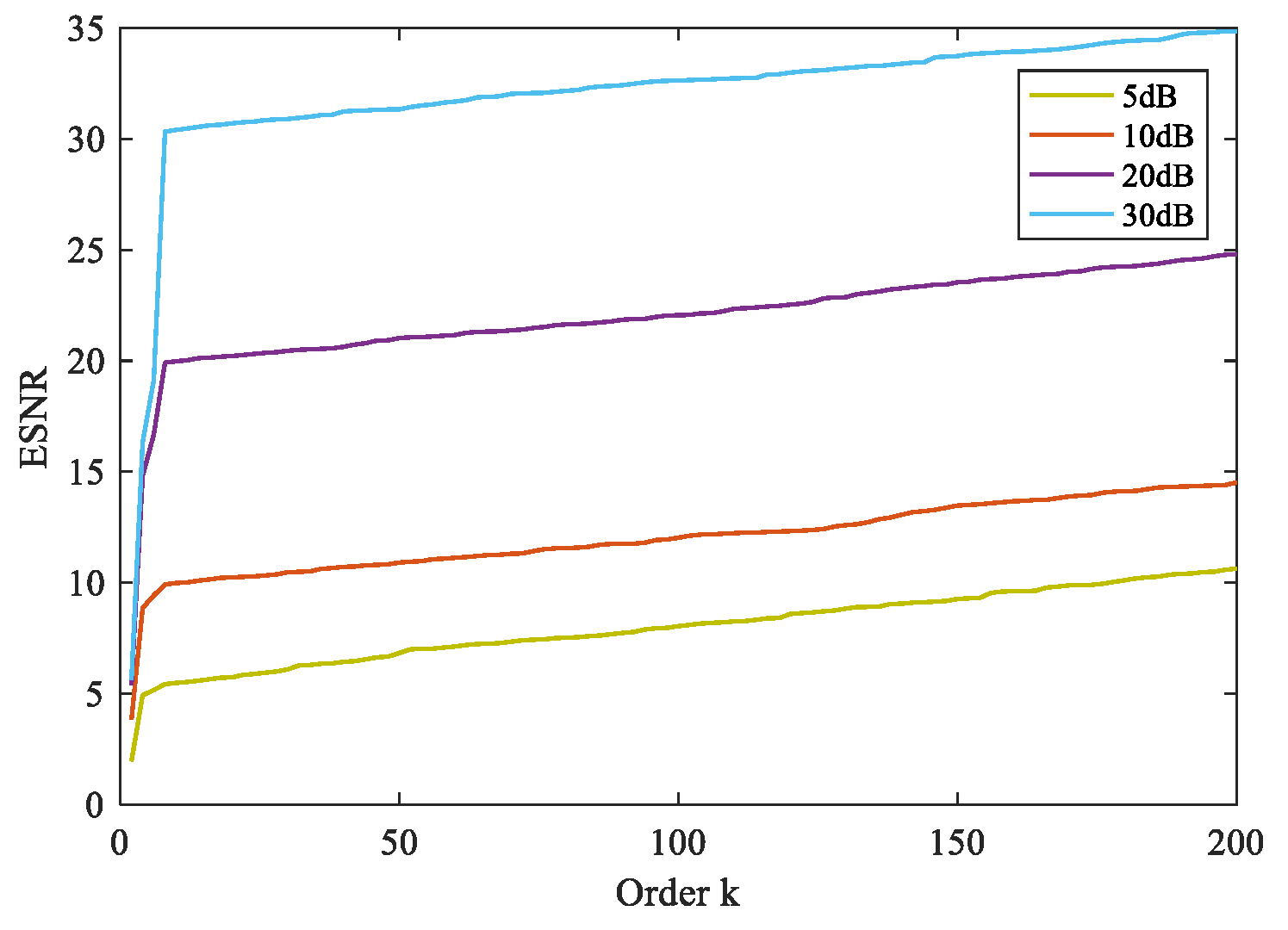
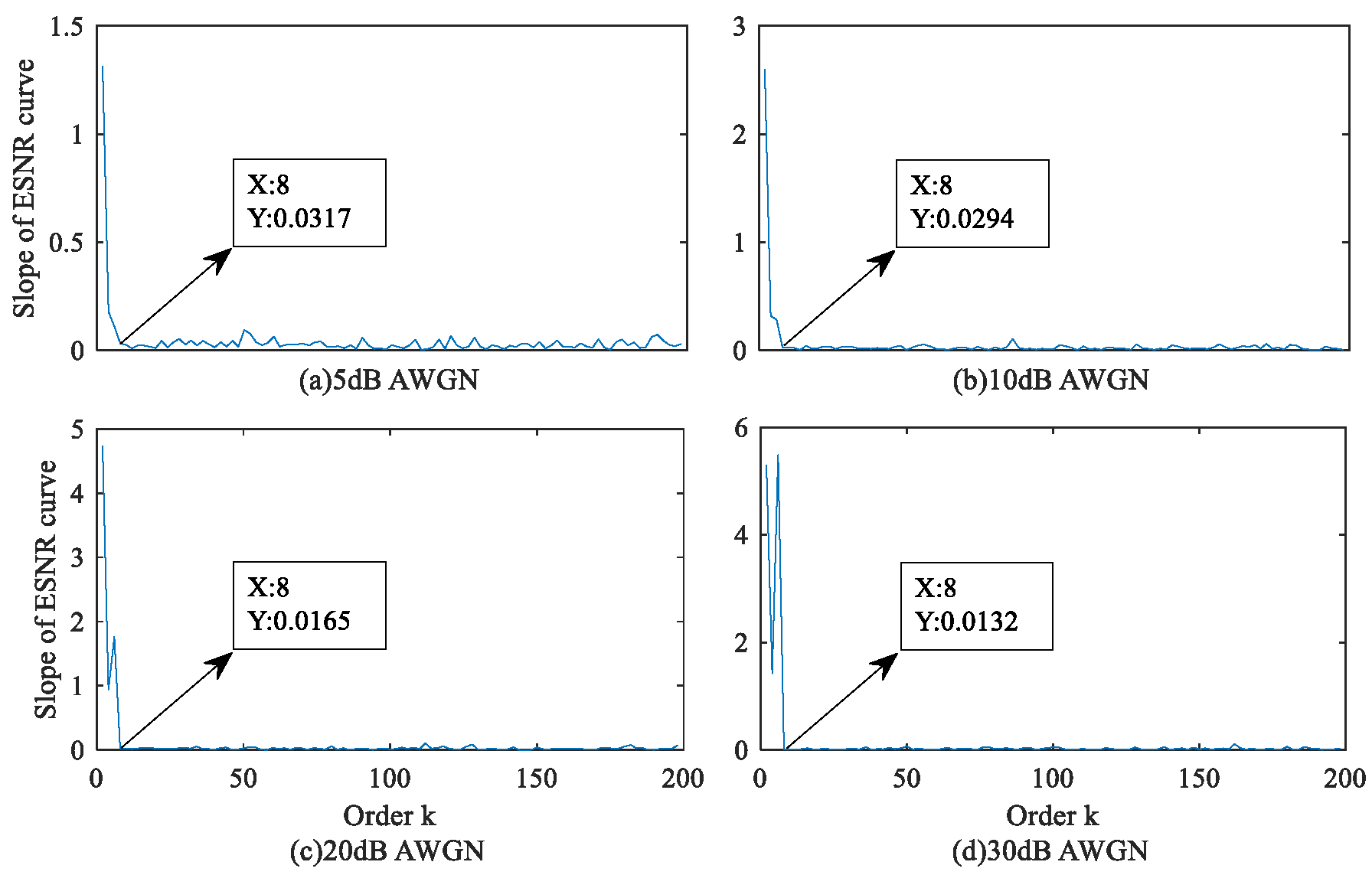
3.2. Adaptive Order Algorithm

The performance of signal denoising is generally evaluated quantitatively via Root Mean Square Error (RMSE) and SNR, and the principle of the proposed adaptive order determination algorithm is closely related to the latter. As such, the definitions of RMSE and SNR are first introduced in the following section. RMSE is defined as

$$RMSE=\sqrt{\frac{1}{N}\sum _{i=1}^N{\left[S^{\prime }\left(i\right)-S\left(i\right)\right]}^2},$$

(4)

and SNR is defined as

$$SNR=10\mathit{lg}\left(\frac{\sum _{i=1}^N{S\left(i\right)}^2}{\sum _{i=1}^N{E\left(i\right)}^2}\right),$$

(5)

where $S^{\prime }\left(i\right)$, $S\left(i\right)$ and $E\left(i\right)$ denote the denoised signal, the noiseless signal and the pure noise signal, respectively. After signal denoising, the smaller the RMSE or the larger the SNR, the better the performance of the denoising method.

The SNR calculated by Equation (5) is known as accurate SNR. However, for an actual signal collected, $S\left(i\right)$ and $E\left(i\right)$ are unknown, and accurate SNR cannot be obtained. Therefore, an estimation method is adopted to calculate SNR. Specifically, $S\left(i\right)$ is replaced by $S^{\prime }\left(i\right)$ and $E\left(i\right)$ is replaced by $E^{\prime }\left(i\right)$ ($E^{\prime }\left(i\right)=X\left(i\right)-S^{\prime }\left(i\right)$). Substituting $S^{\prime }\left(i\right)$ and $E^{\prime }\left(i\right)$ into Equation (5), the Estimated Signal-to-Noise Ratio (ESNR) can be obtained:

$$ESNR=10\mathit{lg}\left(\frac{\sum _{i=1}^N{S}^{\prime }{\left(i\right)}^2}{\sum _{i=1}^N{\left|X\left(i\right)-S^{\prime }\left(i\right)\right|}^2}\right).$$

(6)

At present, there is no fixed method for selecting the effective order $k$ in SVD decomposition. The mean value method is commonly used, which computes the mean value of SVD decomposition singular values and sets those below the mean value to zero to determine the order $k$. However, this method is not self-adaptive and is prone to under-denoising. Literature [19] proposes a method to determine the effective order $k$ based on the rate of change in the singular values. This method is effective when the noise intensity is low, but underperforms in the case of high noise intensity as changes in singular values representing noise and noiseless signals become less significant and the effective order $k$ becomes harder to determine. According to the decomposition characteristics of SVD and a large number of existing studies, the number of eigenvalues representing useful signals is twice the number of frequency components in the useful signals. Thus, the optimal order for denoising should be twice the number of frequency components in non-noisy signals. In this paper, different orders $k$ ($k$ is even) are selected for SVD denoising of the sample signal. Based on Equations (5) and (6), the accurate SNR and ESNR of the signal after denoising are calculated, and the curves of accurate SNR and ESNR against different orders are plotted. According to the characteristics of the curves, an adaptive order determination algorithm is proposed to determine the optimal order value $k$.

To illustrate the adaptive order algorithm, an electric power signal containing a fundamental wave, harmonics and interharmonics is constructed as follows.

$$\begin{array}{c}y=8.7\mathit{cos}\left(50\pi t+0.167\pi \right)+14.2\mathit{cos}\left(100\pi t+0.25\pi \right)\\ +4.5\mathit{cos}\left(310\pi t+0.2\pi \right)+1.5cos(500\pi t+0.333\pi ).\end{array}$$

(7)

The fundamental wave of signal y is at 50 Hz, containing harmonics at a 250 Hz frequency and interharmonics at 25 Hz and 155 Hz frequencies. A 20 dB white Gaussian noise e is applied to signal y to obtain the noisy signal $Y=y+e$. The adaptive order algorithm also applies to electric power signals with different amplitudes, frequency and phases without loss of generality.

Different order values $k$ ($k$ is even) are selected for SVD denoising of signal Y. Applying Equations (5) and (6), the curves of SNR and ESNR against different order values and their slopes are plotted in Figure 2.

Figure 2a illustrates the curve of accurate SNR obtained by Equation (5). When the order $k$ is less than eight, the system is in a state of over-denoising, where noise signals are filtered out along with a large number of noiseless signals. As $k$ increases from two to eight, the filtered noiseless signal decreases rapidly and the SNR increases rapidly. When $k=8$, SNR reaches its maximum and SVD has optimal denoising effect. At this point, the noiseless signal is maximally retained, whereas the noisy signal is maximally filtered out. As $k$ increases further, the system enters the state of under-denoising, as the filtered noise signal decreases and the SNR gradually drops.

Figure 2b presents the curve of ESNR obtained by Equation (6). For $k$ of less than eight, the system is in a state of over-denoising. When $k$ increases from two to eight, the over-denoising state diminishes and ESNR increases rapidly. When $k>8$, the system enters the state of under-denoising, while ESNR continues to increase gently from this point onwards. This can be explained by Equation (6), where the noise signal not filtered in the under-denoising state is retained in the signal after denoising, ${\mathrm{S}}^{\mathrm{\prime }}\left(i\right)$. This leads to a gentle increase of $S^{\prime }\left(i\right)$ and a gentle decrease of $\left|X\left(i\right)-S^{\prime }\left(i\right)\right|$ with an increasing $k$, thus resulting in a gentle increase in ESNR.

From Figure 2a,b, both the curves of accurate SNR and ESNR are divided into two apparent stages, with the turning points in both being $k=8$. Moreover, it can be deduced from Figure 2a that $k=8$ is the optimal order for SVD denoising. Hence, in practical applications, this optimal order can be determined by finding the state turning point of the ESNR curve.

Figure 2c depicts the change in slope of the curve in Figure 2a. It can be observed that before point $k=8$, the accurate SNR curve has a positive curve, SNR increases rapidly, and SVD’s denoising capability is continuously enhanced. From $k=8$ onwards, however, the slope is less than or equal to zero, and SNR gradually declines, with the denoising capability of SVD constantly weakened.

Similarly, Figure 2d depicts the change in slope corresponding to the curve in Figure 2b. It can be seen that before $k=8$, the ESNR curve has a positive slope and increases rapidly. After $k=8$, the slope becomes positive and close to zero, and ESNR increases gently.

Hence, it can be inferred that the change in slope of the accurate SNR curve demonstrates a consistent pattern with that of the ESNR curve, which further corroborates that the change in the ESNR can provide a basis for the selection of effective order $k$, and the state turning point of the ESNR can be found based on the slope of the ESNR curve. Therefore, the following equation can be established according to the characteristics of the slope of the ESNR curve:

$$\left\{\begin{array}{c}f\left(k\right)=\frac{1}{2}\left[ESNR\left(k+2\right)-ESNR\left(k\right)\right],\frac{k}{2}\in N^{+}\hfill \\ k_{opt}=arg\left[f\left(k\right)<0.1\right]\end{array},\right.$$

(8)

where $f\left(k\right)$ represents the slope of the ESNR curve and $k_{opt}$ denotes the solution of $f\left(k\right)$ when inequality $f\left(k\right)<0.1$ holds for the first time, which is essentially the optimal order for SVD denoising. In short, when applying the SVD denoising algorithm, the optimal order $k$ of SVD denoising can be determined adaptively according to Equation (8), thereby avoiding the influence of different noise intensities on the SVD denoising performance and achieving higher adaptability and robustness.

3.3. Prony Algorithm

The Prony algorithm assumes that data $x\left(n\right)$ to be analyzed is composed of $p$ exponential functions with arbitrary amplitudes, phases, frequencies and attenuation factors. Its mathematical model is given by

$$\widehat{x}\left(n\right)=\sum _{i=1}^p{b}_i{z}_i^n,n=\mathrm{0,1},2,\cdots ,N-1,$$

(9)

where $b_i=A_i\exp \left(j{\theta }_i\right)$, $z_i=\exp [\left({\alpha }_i+j{2\pi f}_i\right)∆t]$, and $\widehat{x}\left(n\right)$ is the fitting value of $x\left(n\right)$; $A_i,f_i,{\theta }_i \mathrm{and} {\alpha }_i$ are the amplitude, frequency, initial phase angle and attenuation factor, respectively; $∆t$ is the sampling interval. Equation (9) can be written in a matrix form as follows:

$$\widehat{\mathit{x}}=\mathit{z}\mathit{b},$$

(10)

where

$$\widehat{\mathit{x}}={\left[\begin{array}{ccc}\widehat{x}\left(0\right)& \begin{array}{cc}\widehat{x}\left(1\right)& \cdots \end{array}& \widehat{x}\left(N\right)\end{array}\right]}^T,\mathit{z}=\left[\begin{array}{ccc}\begin{array}{cc}1& 1\\ z_1& z_2\end{array}& \cdots & \begin{array}{c}1\\ z_P\end{array}\\ \begin{array}{cc}⋮& ⋮\end{array}& \ddots & ⋮\\ \begin{array}{cc}{z}_1^{N-1}& z_2^{N-2}\end{array}& \cdots & z_P^{N-1}\end{array}\right],\mathit{b}=\left[\begin{array}{c}{b}_1\\ \begin{array}{c}{b}_2\\ ⋮\end{array}\\ b_p\end{array}\right].$$

(11)

The following objective function is constructed to minimize the fitting error:

$$min\epsilon =\sum _{n=0}^{N-1}{|x\left(n\right)-\widehat{x}(n\left)\right|}^2.$$

(12)

It should be noted that Equation (9) is a homogeneous solution of a linear difference equation with constant coefficients. Thus,

$$\widehat{x}\left(n\right)=-\sum _{i=1}^p{a}_i\widehat{x}\left(n-i\right),p\le n\le N-1.$$

(13)

The error between data $x\left(n\right)$ to be analyzed and fitting data $\widehat{x}\left(n\right)$ can be defined as $e\left(n\right)$:

$$e\left(n\right)=x\left(n\right)-\widehat{x}\left(n\right),n=\mathrm{0,1},2,\cdots ,N-1.$$

(14)

Hence, Equations (13) and (14) provide

$$\begin{array}{ll}x\left(n\right)& =\widehat{x}\left(n\right)+e\left(n\right)=-{\displaystyle \sum _{i=1}^p}{a}_i\widehat{x}\left(n-i\right)+e\left(n\right)\\ & =-{\displaystyle \sum _{i=1}^p}{a}_{i}x\left(n-i\right)+{\displaystyle \sum _{i=0}^p}{a}_{i}e\left(n-i\right),\end{array}$$

(15)

for which one can define $u\left(n\right)=\sum _{i=0}^p{a}_{i}e\left(n-i\right)$. $x\left(n\right)$ can be regarded as the output generated by a p-order autoregressive model excited by error $u\left(n\right)$, and the parameter $a_i$ can be obtained by solving the canonical equation of the model. Substituting $a_i$ into Equation (16) and computing the root of the polynomial yields parameter $z_i$.

$$\sum _{i=0}^p{a}_i{z}^{p-i}=0.$$

(16)

From Equations (10) and (11), the least square method is used to solve the matrix, and parameter $b_i$ can be obtained. The least square solution is provided by

$$\mathit{b}={\left({\mathit{z}}^H\mathit{z}\right)}^{-1}{\mathit{z}}^H\widehat{\mathit{x}}.$$

(17)

Finally, harmonic and interharmonic parameters are obtained through the following equations:

$$\left\{\begin{array}{l}\\ A_i=\left|b_i\right|\\ f_i=arctan\left[\frac{Im\left(z_i\right)}{Re\left(z_i\right)}\right]/2\pi ∆t\\ {\theta }_i=arctan\left[\frac{Im\left(b_i\right)}{Re\left(b_i\right)}\right]/2\pi ∆t\\ {\alpha }_i=\frac{Im\left(z_i\right)}{∆t}\end{array},i=\mathrm{1,2},\cdots ,p.\right.$$

(18)

From Equation (9), when performing fitting analysis on data $x\left(n\right)$ using the Prony algorithm, under the assumption that $x\left(n\right)$ is composed of p exponential functions, p sets of data are involved in the results calculated from Equation (18). Each set of data consists of $A_i,f_i,{\theta }_i\mathrm{and}{\alpha }_i$. They contain both non-false components characterizing useful signal parameters and false components characterizing noise signal parameters. Hence, these non-false components need to be accurately screened from these data.

3.4. Data Filtering

While using the Prony algorithm for signal detection, a larger model order $p$ is usually selected due to the presence of noise in the signal. The fitting result contains many false components which are used to fit the noise in the signal. If the noise is weak, the amplitude of these false components is generally small and attenuates quickly. When the noise is strong, the amplitude of these false components may surpass that of the non-false components, which interferes with the deduction of the non-false components. Therefore, it is imperative to screen the data fitted by the Prony algorithm to determine the non-false components. To this end, this paper proposes a data screening method based on dominant factor ($\mu$). The dominant factor is expressed as

$${\mu }_i=\left|\frac{A_i}{{\alpha }_i}\right|,i=\mathrm{1,2},\cdots ,p,$$

(19)

where $A_i$ is the amplitude of each frequency component; ${\alpha }_i$ is the attenuation factor of each frequency component; $p$ is the model order of the Prony algorithm; ${\mu }_i$ denotes the dominant factor of each frequency component in the fitting result, representing the leading role of each frequency component in the signal. Once the noise in the signal is effectively filtered out, the false component representing the noise no longer plays a leading role, and its leading factor becomes close to zero. Meanwhile, the non-false component representing the noiseless signal plays a leading role with its dominant factor greater than one. This leads to the following expression:

$$\left\{\begin{array}{l}{\mu }_i>1\\ Result=[A_i,f_i,{\phi }_i]\end{array}\right.,$$

(20)

where R_opt represents the non-false component screened out. R_opt consists of $A_i,f_i\mathrm{a}\mathrm{n}\mathrm{d}{\phi }_i$, which represent the amplitude, frequency and phase, respectively, and constitute the final detection results of harmonic and interharmonic signal parameters in electric power signals by the proposed method. According to Equation (20), when the dominant factor is greater than one, the frequency component plays a leading role in the signal and is a non-false component that is to be retained.

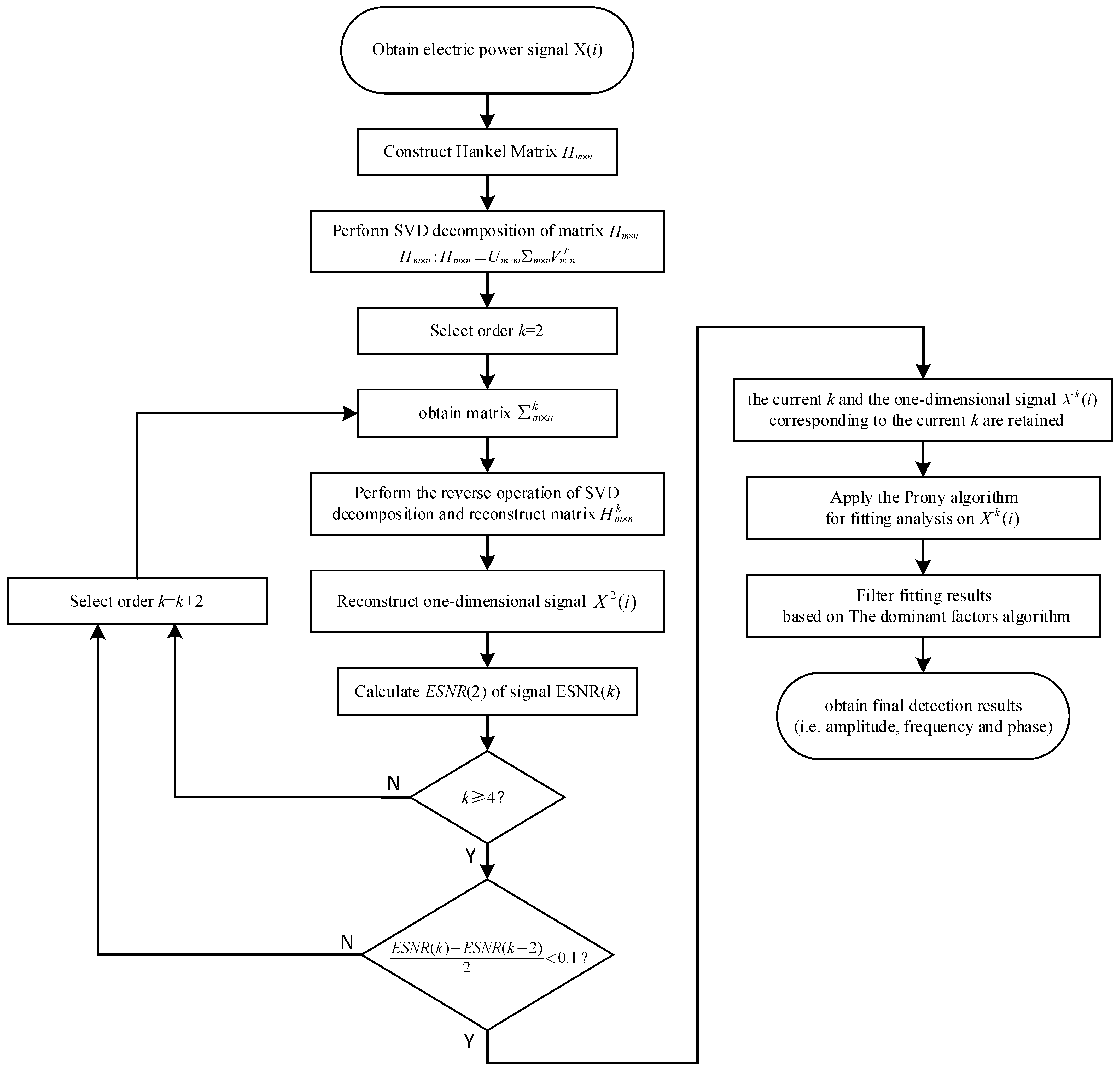
3.5. Algorithm Flow

The overall process of this algorithm can be described as follows (Algorithm 1).

Algorithm 1: The Proposed Algorithm

1: Obtain electric power signal $\mathrm{X}\left(i\right)=[x\left(1\right),x\left(2\right),\cdots ,x\left(\mathrm{N}\right)]$.

2: Construct electric energy signal $\mathrm{X}\left(i\right)$ as Hankel matrix ${\mathit{H}}_{m\times n}$.

3: Perform SVD decomposition of matrix ${\mathit{H}}_{m\times n}$: ${\mathit{H}}_{m\times n}={\mathit{U}}_{m\times m}{\mathsf{\Sigma }}_{m\times n}{\mathit{V}}_{n\times n}^T$.

4: Select order $k=2$ of the eigenvalue matrix ${\mathsf{\Sigma }}_{m\times n}$ and set all eigenvalues after the second eigenvalue on the diagonal of matrix ${\mathsf{\Sigma }}_{m\times n}$ to zero to obtain matrix ${\mathsf{\Sigma }}_{m\times n}^2$.

5: Perform the reverse operation of SVD decomposition and reconstruct matrix ${\mathit{H}}_{m\times n}^2$ after denoising according to ${\mathit{U}}_{m\times m}{\mathsf{\Sigma }}_{m\times n}^2{\mathit{V}}_{n\times n}^T={\mathit{H}}_{m\times n}^2.$

6: Reconstruct one-dimensional signal ${\mathrm{X}}^2\left(i\right)$ according to matrix ${\mathit{H}}_{m\times n}^2.$

7: Calculate ESNR(2) of one-dimensional signal ${\mathrm{X}}^2\left(i\right)$ according to Equation (6).

8: Select order $k=4$ of the eigenvalue matrix ${\mathsf{\Sigma }}_{m\times n}$ and set all eigenvalues after the fourth eigenvalue on the diagonal of matrix ${\mathsf{\Sigma }}_{m\times n}$ to zero to obtain matrix ${\mathsf{\Sigma }}_{m\times n}^4.$

9: Perform the reverse operation of SVD decomposition and reconstruct matrix ${\mathit{H}}_{m\times n}^4$ after denoising according to ${\mathit{U}}_{m\times m}{\mathsf{\Sigma }}_{m\times n}^4{\mathit{V}}_{n\times n}^T={\mathit{H}}_{m\times n}^4.$

10: Reconstruct one-dimensional signal ${\mathrm{X}}^4\left(i\right)$ according to matrix ${\mathit{H}}_{m\times n}^4.$

11: Calculate ESNR(4) of one-dimensional signal ${\mathrm{X}}^4\left(i\right)$ according to Equation (6).

12: Calculate rate of change between ESNR(4) and ESNR(2) according to $f\left(k\right)=0.5\times \left[ESNR\left(k+2\right)-ESNR\left(k\right)\right]$.

13: If rate of change does not meet $f\left(k\right)<0.1$, order $k=6$ of the eigenvalue matrix ${\mathsf{\Sigma }}_{m\times n}$ is selected, and steps 8–12 are repeated to obtain ESNR(6); rate of change between ESNR(6) and ESNR(4) is calculated; order $k$ is chosen by adding two to the previous $k$ value.

14: When $f\left(k\right)<0.1$ holds for the first time, the current $k$ (i.e., optimal order for SVD denoising) and the one-dimensional signal ${\mathrm{X}}^k\left(i\right)$ corresponding to the current $k$ (i.e., electric energy signal after denoising) are retained.

15: Apply the Prony algorithm for fitting analysis on ${\mathrm{X}}^k\left(i\right)$.

16: Calculate the dominant factors of each frequency component in the fitting results according to Equation (19) and screen fitting results through Equation (20) to obtain the final detection results of harmonic and interharmonic signal parameters in the electric power signal (i.e., amplitude, frequency and phase).

The flowchart of this algorithm is shown in Figure 3.

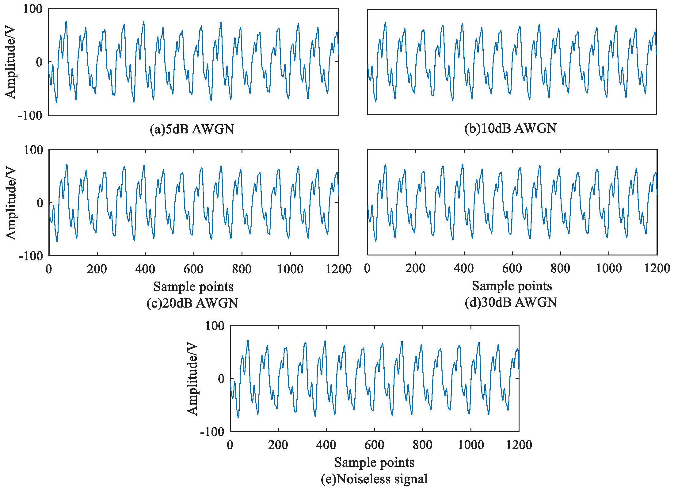
4. Simulation Analysis

To verify the effectiveness of the proposed method for the detection of harmonics and interharmonics in power systems, a simulation analysis is carried out in this study. An electric power signal containing fundamental waves, harmonics and interharmonics is constructed according to literature [22].

$$\begin{array}{cc}y\left(t\right)& =50.4e^{-0.095t}\mathit{cos}\left(100\pi t+0.4\pi \right)+25e^{-0.32t}\mathit{cos}\left(300\pi t+0.6\pi \right)\\ & +8.5e^{-1.54t}\mathit{cos}\left(276\pi t+0.8\pi \right)+6.2e^{-0.34t}\mathit{cos}\left(700\pi t+0.89\pi \right).\end{array}$$

(21)

The sample frequency is set as 4000 Hz, the number of sample points is set as 1200, and the order of the Prony model is set as 0.1 N, (i.e., $p=120$). The “awgn” function is used to apply 5 dB, 10 dB, 20 dB and 30 dB white Gaussian noise to the signals, respectively, resulting in four groups of signals with noise. The waveforms of the four groups of signals with noise and the noiseless signal are shown in Figure 4. The harmonics and interharmonics of the four groups of noisy signals are detected by the Algorithm 1.

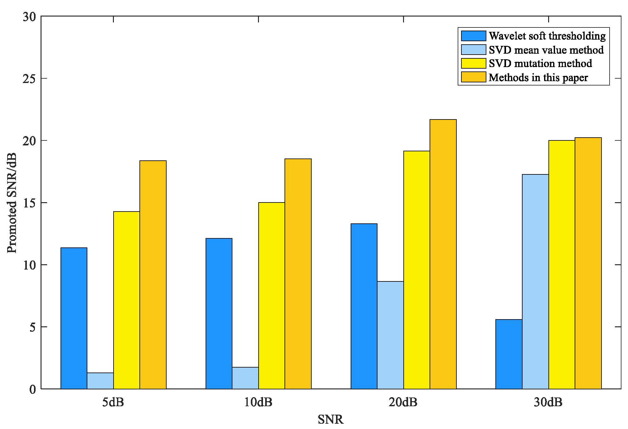
4.1. Signal Denoising

To begin with, four groups of signals with noise are denoised under different orders $k$ as described in Section 3.1 and Section 3.2. Their ESNR curves after denoising are obtained according to Equations (5) and (6) and are plotted in Figure 5. The variations of the slopes of the ESNR curves are shown in Figure 6.

As can be seen from Figure 5, the ESNR curves of the four groups of noisy signals are divided into two apparent stages, and the order of turning points of the two stages is the effective order. From Figure 6, the slopes of the ESNR curves are approximately zero when the order is greater than or equal to eight. According to the principle of the adaptive order determination algorithm and Equation (8), the effective orders of the four groups of noisy signals are all selected as eight. On the other hand, the noiseless signal $y\left(t\right)$ is composed of four frequency components, suggesting that the optimal order of SVD denoising is eight. This example highlights the adaptive order algorithm’s ability to find the optimal order of SVD denoising under different noise intensities and thus its strong adaptability.

Figure 7 presents the waveforms of the four groups of denoised signals and the noiseless signal. Noticeably, the denoised signal maximally resembles its noiseless counterpart under different noise intensities with no apparent signal distortion. This indicates that the denoising is effective and stable.

Next, the proposed denoising method is compared with the SVD mean method, the SVD mutation method and the wavelet soft thresholding method. According to Equations (4) and (5), adopting SNR and RMSE as the evaluation metrics and with reference to Equations (4) and (5), their denoising performance is evaluated in Figure 8 and Figure 9.

It can be seen from Figure 8 and Figure 9 that the commonly used wavelet soft thresholding method is able to denoise the signals to a certain extent. Signals of 5–20 dB see a 12 dB increase in the SNR on average, and the 30 dB signal has its SNR increased by around 5 dB, with a large RMSE error. When applying the SVD mean value method to the 30 dB signal, the singular value of the SVD decomposition is very small, and its mean value is dominated by the noiseless signal. As a result, the SVD mean value method can remove noise well, with SNR increasing by about 17 dB and RMSE close to zero. Yet, as noise gradually increases, the singular value representing noise in SVD decomposition becomes larger, and the mean of the singular value is increasingly dominated by noise. Consequently, the SNRs of 5 dB and 10 dB signals are hardly improved after denoising, and the noise can barely be removed. In this case, the RMSE error is excessively large, and the SVD mean method fails. The SVD mutation method is on par with the proposed method on the 30 dB signal, where the SNR is improved by about 20 dB. Nevertheless, when the noise in the signal gradually increases, the singular value representing the noise becomes larger. This is when the mutation between the singular value representing the noise and the noiseless signals is weakened, and the denoising performance deteriorates. For the signals of 5 dB to 20 dB, its resultant SNR improvement is 4 dB lower than that of the proposed method. Compared with the three considered methods, the denoising performance of the proposed method is less affected by noise, and the selected order $k$ is more effective. The proposed method increases the SNRs of the four groups of noisy signals by about 20 dB on average and results in the minimum RMSE, manifesting strong adaptability and robustness.

4.2. Detecting Harmonic and Interharmonic Signals

The Prony algorithm is highly sensitive to noise and its fitting accuracy can be easily compromised. It can have many false components in its fitting results, and the amplitude of certain false components may be higher than that of non-false components, making it difficult to get rid of the spurious components. These drawbacks lead to low reliability of the Prony algorithm in practical application. In this section, the Prony algorithm and the proposed method are applied, respectively, to detect harmonics and interharmonics of the four groups of noisy signals. Some of the detection results are presented in

Table 1. Detection results obtained by the Prony algorithm and the proposed method.

Before Denoising SNR	Prony Algorithm				The Proposed Method
	Amplitude /V	Frequency /Hz	Phase/°	Attenuation Factor	Amplitude /V	Frequency /Hz	Phase/°	Attenuation Factor	Dominant Factor
5 dB	368.3924	779.0909	34.1670	−538.5595	50.2379	49.9946	71.7320	−0.1279	392.7905
	149.8316	793.3605	179.6763	−135.9869	24.8951	149.9963	107.1586	−0.3297	75.5083
	59.1708	30.6002	102.8747	−141.3244	8.7083	137.8659	141.9504	−0.1860	47.3565
	50.6543	50.0278	70.6035	−0.1404	6.1268	349.9532	160.7258	−1.2100	5.0635
	36.9181	149.7132	123.6631	−4.0898	2.5826	319.0668	44.8012	−66.7384	0.0522
	31.0460	287.0820	143.5194	−122.5444	1.7748	343.3577	170.2391	−15.2113	0.1167
	23.1498	355.5101	92.8171	−67.1172	1.5152	198.5234	109.4213	−54.4115	0.0278
	22.8510	188.2917	171.7149	−53.1641	1.4871	258.8410	6.7160	−72.0078	0.0207
10 dB	292.7002	184.8522	153.7994	−740.6918	50.4065	49.9963	72.3137	−0.1008	500.0645
	83.3545	734.6794	103.8009	−411.8509	25.1007	150.0043	107.9841	−0.2800	89.6454
	52.8242	49.9528	74.4297	−0.3731	8.6343	137.9901	143.9876	−1.7352	5.0336
	41.6969	182.4927	29.8205	−595.6980	6.2607	350.0049	160.4478	−0.6625	9.7520
	40.7923	150.1790	99.2792	−4.8672	6.3925	512.2301	14.6780	−898.9631	0.0071
	11.2334	350.1351	163.7297	−12.0463	4.0890	327.4281	52.4083	−227.2411	0.0180
	9.2335	135.9086	122.6909	−43.8386	2.9818	478.3799	164.9383	−413.5335	0.0072
	6.4724	240.6855	1.8089	−49.8908	1.3560	929.1278	46.8287	−195.8049	0.0069
20 dB	85.2741	579.5170	54.9866	−620.8631	50.3869	49.9994	72.0592	−0.0903	557.9945
	50.9132	50.0017	71.9242	−0.1827	25.0419	149.9997	108.0167	−0.2814	88.9904
	37.7624	121.4600	40.8577	−171.2520	8.5718	138.0054	143.8190	−1.5998	5.3580
	27.2627	150.0270	106.7519	−0.9241	6.3054	350.0015	160.4092	−0.4510	13.9809
	17.0381	138.8344	58.7591	−105.0894	1.4600	113.8934	180.0000	−586.8984	0.0107
	11.6107	383.2363	94.7416	−118.2871	0.6265	103.0310	38.6674	−716.9492	0.0009
	7.3542	349.9924	162.0018	−1.5335	0.6158	803.2629	61.8563	−808.0462	0.0008
	3.9676	349.7109	146.4665	−63.7995	0.4230	457.5418	90.0185	−303.4712	0.0014
30 dB	49.8536	50.0016	71.8437	−0.0719	50.3943	49.9998	72.0175	−0.0937	537.8260
	24.6096	149.9883	107.9125	−0.5973	24.9830	150.0001	107.9953	−0.3016	82.8349
	14.1595	545.9081	107.3173	−451.7063	8.4957	137.9972	144.1354	−1.5331	5.5415
	11.9603	137.9193	148.3649	−5.7621	6.2310	350.0006	160.1573	−0.3791	16.4363
	5.9992	349.9786	161.4551	−0.4599	1.4133	169.9994	102.9522	−414.4383	0.0034
	4.5662	374.9733	92.9159	−235.3819	0.2308	68.4535	174.9564	−100.4966	0.0023
	2.1265	184.1879	97.0321	−76.6287	0.1756	105.6480	174.5260	−100.9045	0.0017
	0.8449	49.7807	152.5392	−50.4207	0.1705	350.6978	35.1884	−102.1557	0.0017

. The dominant factors corresponding to each frequency component in the detection results obtained by the proposed method were calculated according to Equation (19) and are provided in Table 1.

Simulation signal $y\left(t\right)$ is known to comprise four frequency components at 50 Hz, 150 Hz, 138 Hz and 350 Hz, respectively. The corresponding amplitudes are 50.4 V, 25 V, 8.5 V and 6.2 V and the corresponding phases are 72°, 108°, 144° and 160.2°.

In Table 1, for the harmonic detection results of the 5 dB noisy signal, the Prony algorithm merely detects the two frequency components at 50.0278 Hz and 149.7132 Hz, both close to the simulation signal. However, the corresponding amplitudes are 50.6543 V and 36.9181 V, respectively, which greatly deviate from the actual values. In contrast, the proposed method detects the frequency components at 49.9946 Hz, 149.9963 Hz, 137.8659 Hz and 349.9532 Hz, respectively, all very close to the simulation signal. Meanwhile, the corresponding amplitudes of the four frequency components are 50.2379 V, 24.8951 V, 8.7083 V and 6.1268 V, and the corresponding phases are 71.7320°, 107.1586°, 141.9504° and 160.7258°. The amplitudes and phases of the four frequency components are also significantly close to the actual parameters of the simulation signal.

For the 10 dB noisy signal, the Prony algorithm only detects three frequency components close to the simulation signal, namely 49.9528 Hz, 150.1750 Hz and 350.1351 Hz. The corresponding amplitudes are 50.9132 V, 27.2627 V and 7.3542 V, which are significantly different from the actual values. By contrast, the proposed method detects four frequency components at 49.9963 Hz, 150.0043 Hz, 137.9901 Hz and 350.0049 Hz, which are very similar to those of the simulation signal. The corresponding amplitudes of the four frequency components are 50.4065 V, 25.1007 V, 8.6343 V and 6.2607 V, and the corresponding phases are 72.3173°, 107.9841°, 143.9876° and 160.4478°. Hence, the amplitudes and phases of the four frequency components also closely aligned with the parameters of the simulation signal.

As for the harmonic detection results of the 20 dB noisy signal, the Prony algorithm detects five frequency components similar to the simulation signal, namely 50.0017 Hz, 150.0270 Hz, 138.8344 Hz, 349.9924 Hz and 349.7109 Hz, but their corresponding amplitudes also significantly differ from the actual values. Meanwhile, the proposed method detects the components at 49.9994 Hz, 149.9997 Hz, 138.0054 Hz and 350.0015 Hz, all very similar to those of the simulation signal. The corresponding amplitudes of the four frequency components are 50.3869 V, 25.0419 V, 8.5718 V and 6.3054 V, and the corresponding phases are 72.0592°, 108.0167°, 143.8190° and 160.4092°. The amplitudes and phases of the four frequency components are also significantly close to the parameters of the simulation signal.

Finally, for the 30 dB noise signal, the Prony algorithm detects four frequency components similar to those of the simulation signal, namely 50.0016 Hz, 149.9883 Hz, 137.9193 Hz and 349.9786 Hz. The corresponding amplitudes are 49.8536 V, 24.6096 V, 11.9603 V and 5.9992 V. Except for 11.9603 V, other amplitudes are close to the actual values. The corresponding phases are 71.8437°, 107.9125°, 148.3649° and 161.4551°, which are close to the actual values. In comparison, the proposed method detects the components at 49.9998 Hz, 150.0001 Hz, 137.9972 Hz and 350.0006 Hz, which are very similar to those of the simulation signal. The corresponding amplitudes of the four frequency components are 50.3943 V, 24.9830 V, 8.4957 V and 6.2310 V, and the corresponding phases are 72.0175°, 107.9953°, 144.1354° and 160.1573°. The amplitudes and phases of the four frequency components closely match the parameters of the simulation signal.

It can be noted that in the detection results of the 5 dB, 10 dB and 20 dB signals, the Prony algorithm detects false components far larger than those of the true amplitude, such as 368.3924 V and 149.8316 V in the detection results of the 5 dB signal, 292.7002 V, 83.3545 V in the 10 dB signal, and 85.2741 V in the 20 dB signal. All these false components have an impact on the selection of actual data.

The detection result of the Prony algorithm deteriorates rapidly with increasing noise intensity, and the number of harmonics and related information in the signal cannot be effectively detected. Even for the 30 dB signal with weak noise intensity, the detection results are not reliable due to large errors in the amplitude and phase angle. For the harmonic detection results of the four groups of noisy signals, the proposed algorithm is able to fit closely to the parameters of the simulation signals. By computing the dominant factor of each frequency component in the detection results, it can be noted that the dominant factors of the frequency components close to the simulation signal parameters are far greater than zero, indicating their dominant roles in the signal, whereas those of other frequency components are roughly zero. Combined with dominant factors and Equation (20), the detection results of the proposed method are screened, and the final harmonic detection results and errors of the method are obtained in

Table 2. Detection results and errors of harmonic signals by the proposed method.

Before Denoising SNR	Amplitude /V	Frequency /Hz	Phase/°	Amplitude, Frequency and Phase Errors/%
5 dB	50.2379	49.9946	71.7320	0.3216/0.0108/0.3722
	24.8951	149.9963	107.1586	0.4196/0.0025/0.7791
	8.7083	137.8659	141.9504	2.4506/0.0972/1.4233
	6.1268	349.9532	160.7258	1.1806/0.0134/0.3282
10 dB	50.4065	49.9963	72.3137	0.0129/0.0074/0.4357
	25.1007	150.0043	107.9841	0.4028/0.0029/0.0147
	8.6343	137.9901	143.9876	1.5800/0.0072/0.0086
	6.2607	350.0049	160.4478	0.9790/0.0014/0.1547
20 dB	50.3869	49.9994	72.0592	0.0260/0.0012/0.0822
	25.0419	149.9997	108.0167	0.1676/0.0002/0.0155
	8.5718	138.0054	143.8190	0.8447/0.0039/0.1257
	6.3054	350.0015	160.4092	1.7000/0.0004/0.1306
30 dB	50.3943	49.9998	72.0175	0.0113/0.0004/0.0243
	24.9830	150.0001	107.9953	0.0680/0.0001/0.0044
	8.4957	137.9972	144.1354	0.0506/0.0020/0.0940
	6.2310	350.0006	160.1573	0.5000/0.0002/0.0267

.

It can be seen from Table 2 that the amplitude, frequency and phase of the data results screened by dominant factors are close to respective parameters in the simulation signal, with very small errors. The final harmonic detection results of the four groups of noisy signals are largely consistent with the actual values, where the detection errors in amplitude and phase are mostly within 0.5%. The detected frequencies are particularly accurate, with errors mostly within 0.01%. These results show that the proposed method achieves effective and stable denoising for the four groups of noisy signals with different noise intensities, overcoming the noise sensitivity problem of the Prony algorithm. The proposed method is able to select the non-false components of fundamental, harmonic and interharmonic signals accurately through the dominant factor algorithm.

5. Conclusions

In the context of harmonic and interharmonic detection in power systems, this paper proposes a harmonic and interharmonic detection method based on enhanced SVD denoising and the Prony algorithm. It addresses the Prony algorithm shortcomings, namely its fitting accuracy being highly susceptible to noise and fitting results being difficult to be screened. The proposed adaptive order determination algorithm identifies the optimal order of SVD denoising, thereby mitigating the noise sensitivity problem of the Prony algorithm and achieving optimal removal of noise signal with boosted SVD denoising capability. Moreover, the dominant factor algorithm is proposed to solve the problem of the mixing of false components representing noise and non-false components representing useful signals in the fitting result of the Prony algorithm. Through the proposed dominant factor algorithm, the non-false components can be quickly screened according to the dominant factor. Simulation results show that four groups of noisy signals with SNRs of 5 dB, 10 dB, 20 dB and 30 dB, respectively, are improved by about 20 dB on average upon denoising. These improvements suggest that the proposed method is able to effectively remove the noise components and successfully overcome the Prony algorithm’s poor accuracy in fitting noise signals. The amplitude of the false component in the fitting result of the Prony algorithm is much smaller than that of the non-false component. According to the dominant factor, non-false components are accurately screened out and all fundamental, harmonic and interharmonic components are successfully detected.

Hence, it is experimentally verified that the proposed method possesses remarkable robustness and adaptability under different noise intensities of electric energy signals. Its detection of harmonics and interharmonics is accurate, stable and reliable, which implies that the method is well-suited for the detection of harmonics and interharmonics in power systems under various noise environments.

Finally, compared to the particularly high accuracy of the proposed method for frequency detection in signals, there is still room for improvement in terms of the detection accuracy of amplitude and phase. In the future, it is worthwhile to incorporate neural networks in the current method for higher detection accuracy for amplitude and phase.

References

- Lu, Y.; Xiao, G.; Wang, X.; Blaabjerg, F. Grid Synchronization with Selective Harmonic Detection Based on Generalized Delayed Signal Superposition. IEEE Trans. Power Electron. 2017, 33, 3938–3949. [Google Scholar] [CrossRef]
- Singh, G.K. Power System Harmonics Research: A Survey. Eur. Trans. Electr. Energy Syst. 2009, 19, 151–172. [Google Scholar] [CrossRef]
- Dou, J.W.; Yang, X.Y.; Yang, X.Z. A Power System Harmonic Detection Method Based on Fractional Wavelet Transform. In Proceedings of the CSEE 2022, Montréal, QC, Canada, 14–19 August 2023; pp. 1–9. [Google Scholar]
- Wen, Y.F.; Yang, W.F.; Wang, R.H.; Xu, W.T.; Ye, X.; Li, T. Review and Prospect of Constructing 100% Renewable Energy Power System. In Proceedings of the CSEE 2022, Montréal, QC, Canada, 14–19 August 2023; pp. 1843–1856. [Google Scholar]
- Peretti, L.; Pathmanathan, M.; Haq, O.; Sahoo, S. Robust Harmonic Detection, Classification and Compensation Method for Electric Drives Based on the Sparse Fft and the Mahalanobis Distance. IET Electr. Power Appl. 2017, 11, 1177–1186. [Google Scholar] [CrossRef] [Green Version]
- Su, T.; Yang, M.; Jin, T.; Flesch, R.C.C. Power Harmonic and Interharmonic Detection Method in Renewable Power Based on Nuttall Double-Window All-Phase Fft Algorithm. IET Renew. Power Gener. 2018, 12, 953–961. [Google Scholar] [CrossRef]
- Li, C.; An, Q. Harmonic Detection Algorithm Based on Kaiser Window. In Proceedings of the 2020 IEEE Conference on Telecommunications, Optics and Computer Science (TOCS), Shenyang, China, 11–13 December 2020. [Google Scholar]
- Chauhan, K.; Venkateswara Reddy, M.; Sodhi, R. A Novel Distribution-Level Phasor Estimation Algorithm using Empirical Wavelet Transform. IEEE Trans. Ind. Electron. 2018, 65, 7984–7995. [Google Scholar] [CrossRef]
- Yang, X.; Xie, W. Research of the Power Harmonic Detection Method Based on Wavelet Packet Transform. In Proceedings of the 2010 International Conference on Measuring Technology & Mechatronics Automation, Changsha, China, 13–14 March 2010. [Google Scholar]
- Tang, Z.G.; Li, Y. Research on Improved Adaptive Parameterless Empirical Wavelet Transform in Transformer High Frequency Partial Discharge Current Noise Suppression. Power Syst. Technol. 2022, 1–12. [Google Scholar]
- Shi, J.; Liu, Z. Harmonic Detection Technology for Power Grids Based on Adaptive Ensemble Empirical Mode Decomposition. IEEE Access 2021, 9, 21218–21226. [Google Scholar] [CrossRef]
- Sun, S.; Pang, Y.; Wang, J.; Zhang, C.; Du, T.; Yu, H. EEMD harmonic detection method based on the new wavelet threshold denoising pretreatment. Power Syst. Prot. Control. 2016, 44, 42–48. [Google Scholar]
- Qin, Y. Fast Implementation of Orthogonal Empirical Mode Decomposition and ITS Application into Harmonic Detection. Chin. J. Mech. Eng. 2008, 21, 93. [Google Scholar] [CrossRef]
- Gu, F.-C.; Chang, H.-C.; Chen, F.-H.; Kuo, C.-C.; Hsu, C.-H. Application of the Hilbert-Huang Transform with Fractal Feature Enhancement on Partial Discharge Recognition of Power Cable Joints. IET Sci. Meas. Technol. 2012, 6, 440–448. [Google Scholar] [CrossRef]
- Afroni, M.J.; Sutanto, D.; Stirling, D. Analysis of nonstationary power-quality waveforms using iterative Hilbert Huang transform and SAX algorithm. IEEE Trans. Power Deliv. 2013, 28, 2134–2144. [Google Scholar] [CrossRef]
- Wang, Z.; Asce, A.G.C.F. Recursive Hilbert-Huang Transform Method for Time-Varying Property Identification of Linear Shear-Type Buildings under Base Excitations. J. Eng. Mech. 2012, 138, 631–639. [Google Scholar] [CrossRef]
- Tong, T.; Zhang, X.Y.; Liu, B.W. Analysis of Harmonic and Interharmonic Detection Based on Fourier-based Synchrosqueezing Transform and Hilbert Transform. Power Syst. Technol. 2019, 43, 4200–4208. [Google Scholar]
- Liang, Z.; Liang, J.; Zhang, L.; Wang, C.; Yun, Z.; Zhang, X. Analysis of Multi-Scale Chaotic Characteristics of Wind Power Based on Hilbert-Huang Transform and Hurst Analysis. Appl. Energy 2015, 159, 51–61. [Google Scholar] [CrossRef]
- Hu, Z.J.; Guo, J.Q.; Yu, M.; Du, Z.; Wang, C. The Studies on Power System Harmonic Analysis Based on Extended Prony Method. In Proceedings of the 2006 International Conference on Power System Technology, Chongqing, China, 22–26 October 2006. [Google Scholar]
- Zygarlicki, J.; Zygarlicka, M.; Mroczka, J.; Latawiec, K.J. A Reduced Prony’s Method in Power-Quality Analysis—Parameters Selection. IEEE Trans. Power Deliv. 2010, 25, 979–986. [Google Scholar] [CrossRef]
- Derin, H. Estimating Components of Univariate Gaussian Mixtures Using Prony’s Method. IEEE Trans. Pattern Anal. Mach. Intell. 1987, PAMI-9, 142–148. [Google Scholar] [CrossRef]
- Trudnowski, D.J.; Johnson, J.M.; Hauer, J.F. Making Prony analysis more accurate using multiple signals. IEEE Trans. Power Syst. 1999, 14, 226–231. [Google Scholar] [CrossRef]
- Wang, X.Y.; Bai, X.M.; Song, C.; Mao, Z.J. APU Exhaust Temperature Prediction Based on EMD-LSTM Model. J. Aerosp. Power 2023, 1–8. [Google Scholar] [CrossRef]
- Li, Z.M.; Xu, M.; Pan, T.H.; Chen, W.H. A harmonic detection method for distributed connected grid system by using wavelet transform and HHT. Power Syst. Prot. Control. 2014, 42, 34–39. [Google Scholar]
- Xiong, G.; Wang, B.; Lu, N.X.; Xia, L.; Zhu, Z.J. Time-Frequency Analysis Method Based on Improved Prony Transform and Its Application in Offshore Wind Turbines. Acta Energ. Sol. Sin. 2022, 43, 280–286. [Google Scholar] [CrossRef]
- Wang, M.H.; Li, K.C.; Liu, C.; Wang, W.; Chen, X.Y. Prony-GSO Combined Harmonic Detection Method Based on VMD De-noising. Electr. Meas. Instrum. 2020, 57, 101–107. [Google Scholar]
- Zhang, Q.; Bian, X.; Xu, X.; Huang, R.; Li, H. Analysis of Influencing Factors on Damping Characteristics of Subsynchronous Oscillation Based on Singular Value Decomposition Prony and Principal Component Regression. Trans. China Electrotech. Soc. 2022, 37, 4364–4376. [Google Scholar]