


Debris Flow Classification and Risk Assessment Based on Combination Weighting Method and Cluster Analysis: A Case Study of Debris Flow Clusters in Longmenshan Town, Pengzhou, China


Abstract
:1. Introduction
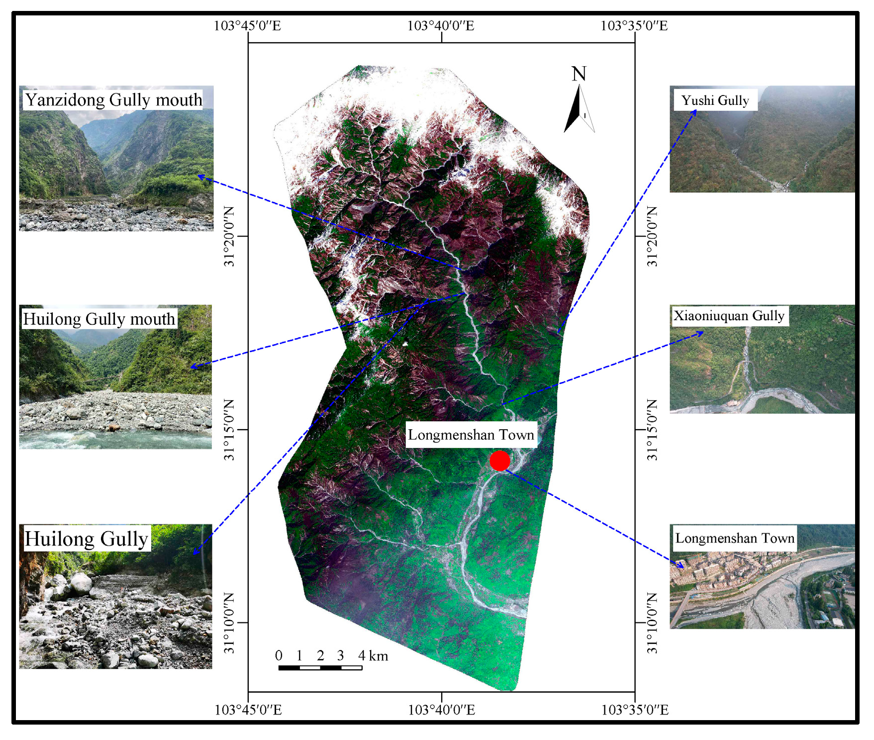
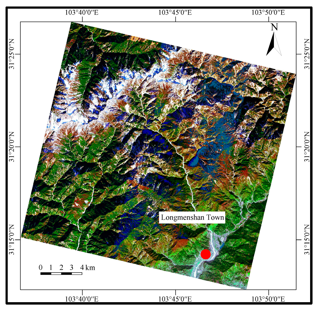
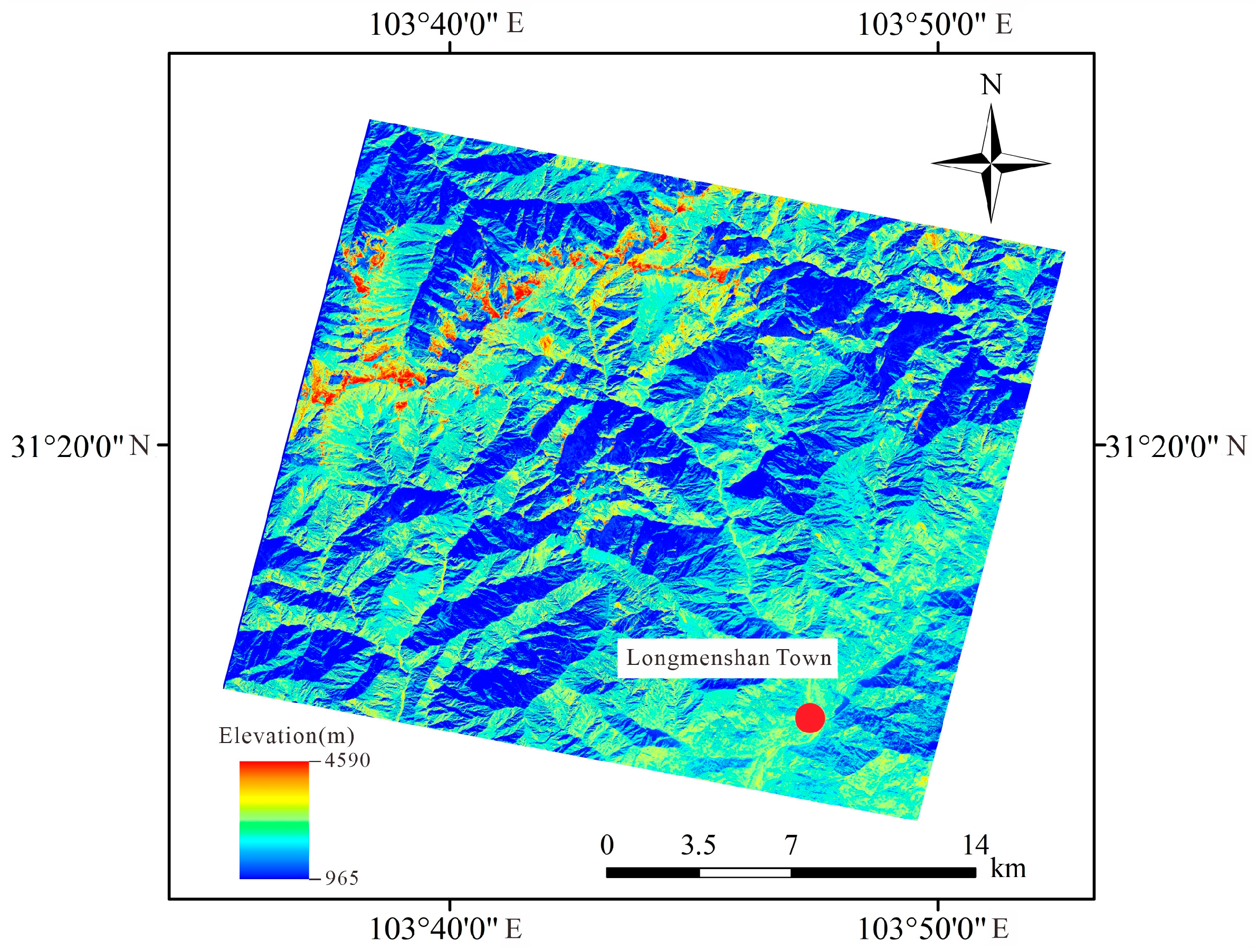
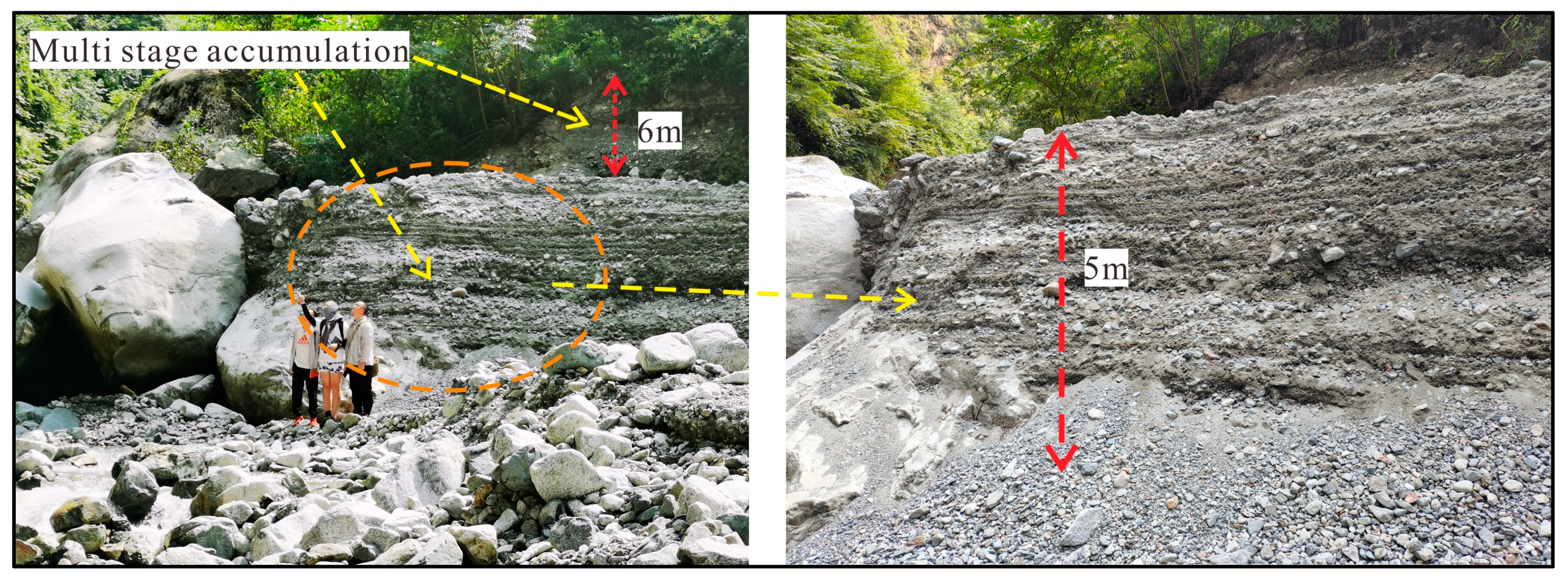
2. Study Area
3. Materials and Methods
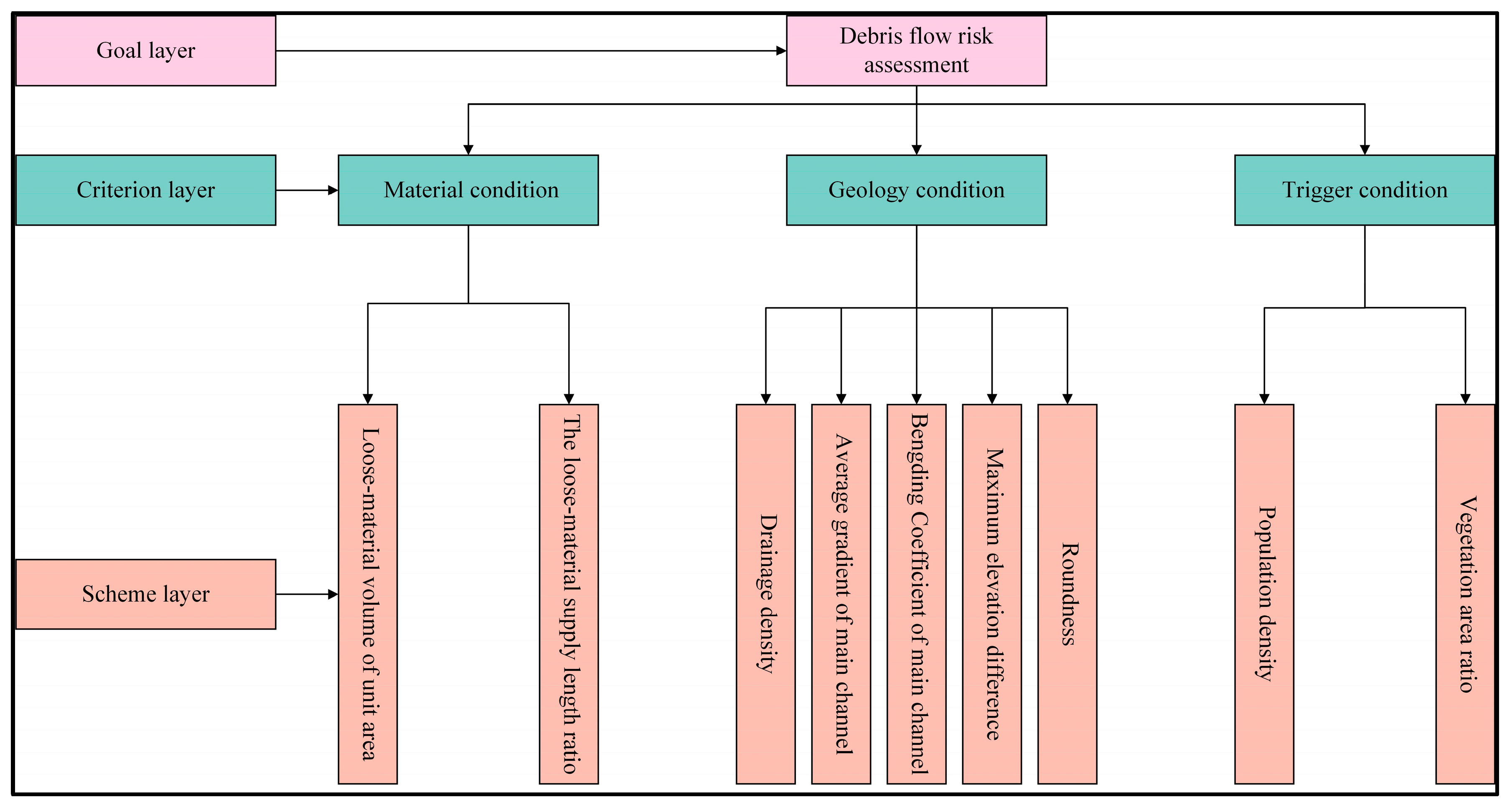
3.1. Indicator Selection
3.2. Combination Weighting Method
3.2.1. CRITIC Method
3.2.2. Analytic Hierarchy Process (AHP)
3.2.3. Combination Weighting Rule
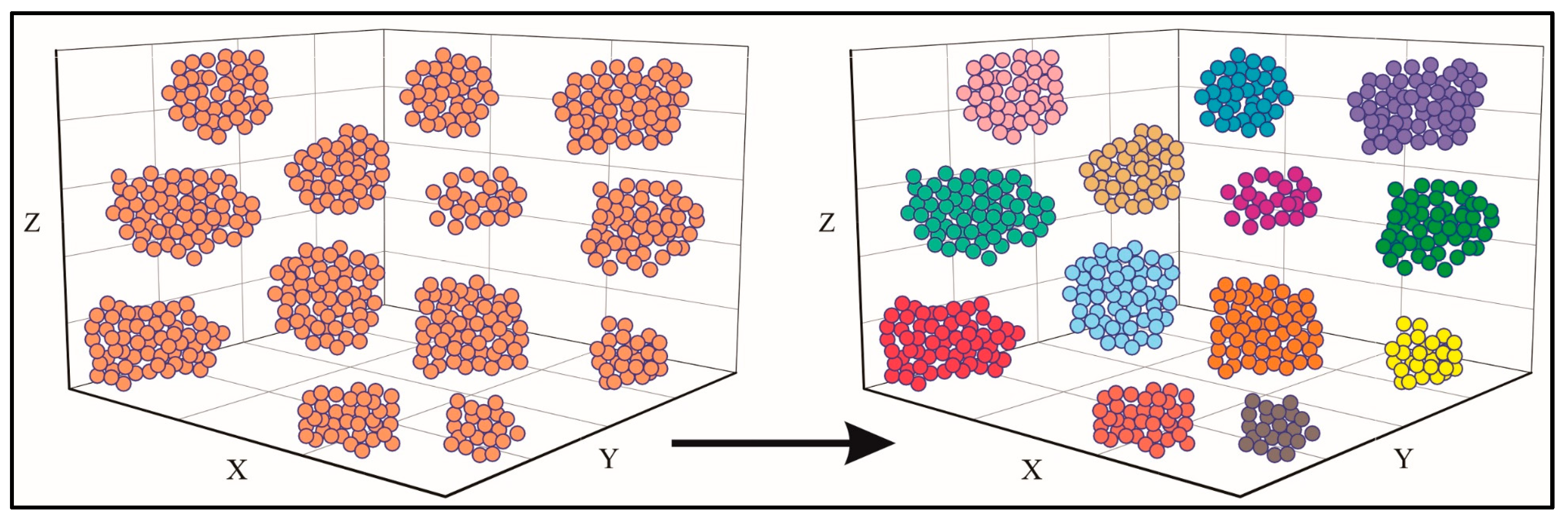
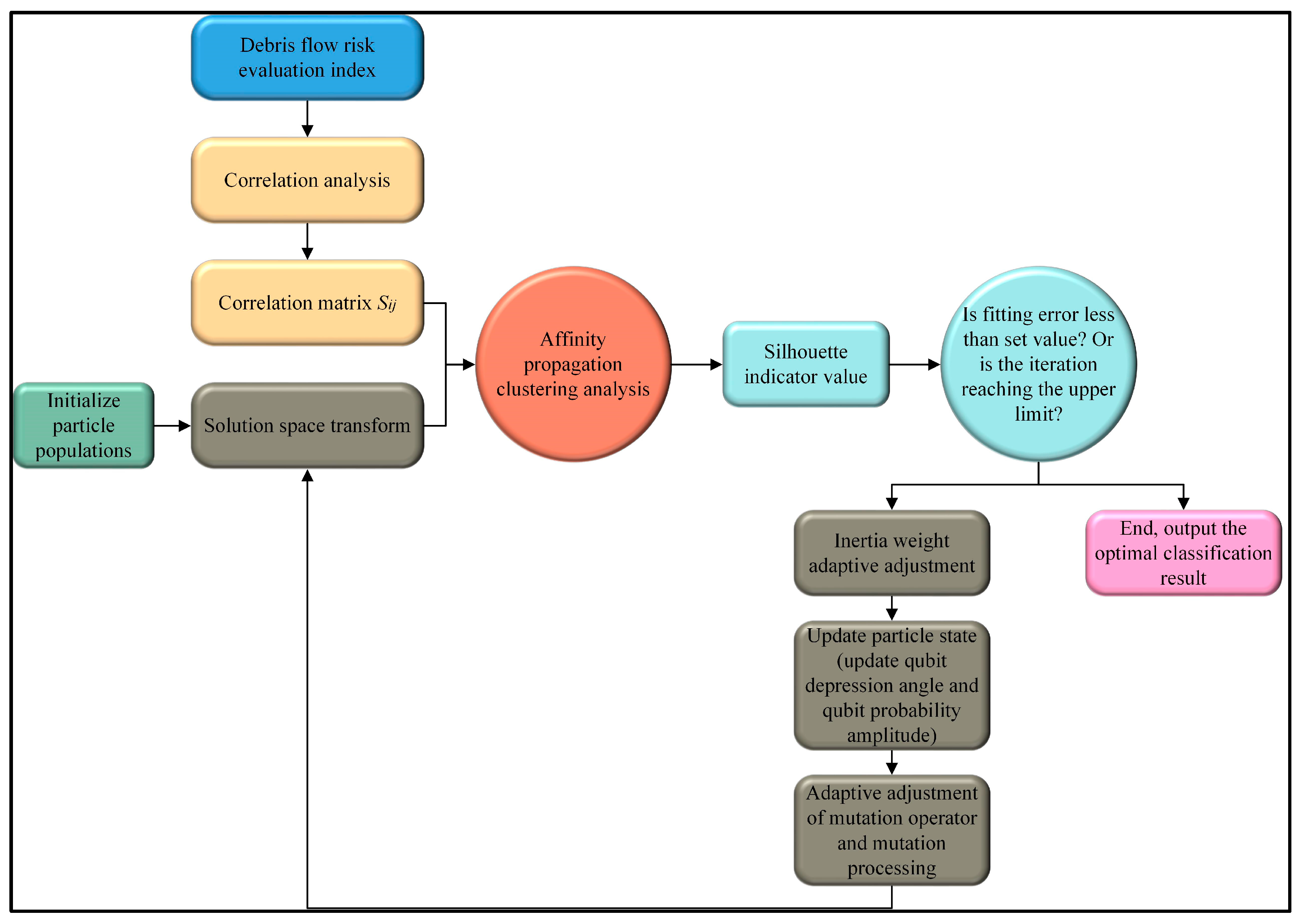
3.3. Cluster Analysis
- (1)
- Calculate data point correlation matrix.
- (2)
- Determining the size of p (Preference) and the number of iterations.
- (3)
- Calculate the responsibility information and the availability information between monitoring points.
- (4)
- Update the responsibility information and availability information.
- (5)
- Calculate the cluster center.
- (6)
- The maximum number of cycles is reached, and the final result is obtained.
3.3.1. Correlation Calculation
3.3.2. Classification and Risk Assessment of Debris Flow
4. Classification and Risk Assessment Results of Debris Flow in the Study Area
4.1. Weight Calculation
4.1.1. Results of the AHP
4.1.2. Results of CRITIC Method
4.1.3. Results of the Combination Weighting Method
4.2. Classification Results of Debris Flow
4.3. Risk Assessment Based on Classification Results
5. Discussion
6. Conclusions
- (1)
- Based on on-site geological surveys, drone images, and multiple remote sensing images, 9 debris flow risk assessment indicators were selected from 14 debris flows in Longmenshan Town, Pengzhou, China. Each indicator’s subjective and objective weights were calculated using hierarchical analysis and CRITIC methods, and the two weights were coupled to obtain the synthetic weights of the evaluation indicators. Based on this, the synthetic evaluation score Di was calculated for each debris flow so that the obtained synthetic evaluation score could scientifically reflect the risk level of each debris flow gully.
- (2)
- This study conducted cluster analysis of 14 debris flows, established the classification model, and classified the debris flows in the study area into four categories. By combining the classification results with synthetic evaluation scores, it was ultimately determined that, among the 14 debris flows in the study area, 3 were extremely dangerous (0.6718 ≤ Di ≤ 0.8301), 4 were highly dangerous (0.3963 ≤ Di ≤ 0.5359), 3 were moderately dangerous (0.2716 ≤ Di ≤ 0.3064), and 4 were low-risk (0.2113 ≤ Di ≤ 0.2692).
Author Contributions
Funding
Institutional Review Board Statement
Informed Consent Statement
Data Availability Statement
Conflicts of Interest
References
- Chen, N.S.; Yue, Z.Q.; Cui, P.; Li, Z.L. A rational method for estimating maximum discharge of a landslide-induced debris flow: A case study from Southwestern China. Geomorphology 2007, 84, 44–58. [Google Scholar] [CrossRef]
- Jomelli, V.; Pavlova, I.; Eckert, N.; Grancher, D.; Brunstein, D. A new hierarchical Bayesian approach to analyse environmental and climatic influences on debris flow occurrence. Geomorphology 2015, 250, 407–421. [Google Scholar] [CrossRef]
- Cardona, F.G.; Giraldo, E.A.; Arango, M.I.; Mergili, M. Regional and detailed multi-hazard assessment of debris-flow processes in the Colombian Andes. In Proceedings of the EGU General Assembly 2021, Online, 19–30 April 2021. [Google Scholar] [CrossRef]
- Cabral, V.; Reis, F.; Veloso, V.; Ogura, A.; Zarfl, C. A multi-step hazard assessment for debris-flow prone areas influenced by hydroclimatic events. Eng. Geol. 2023, 313, 106961. [Google Scholar] [CrossRef]
- Joshi, M.; Rajappan, S.; Rajan, P.P.; Mathai, J.; Sankar, G.; Nandakumar, V.; Kumar, V.A. Weathering controlled landslide in Deccan traps: Insight from Mahabaleshwar, Maharashtra. J. Geol. Soc. India 2018, 92, 555–561. [Google Scholar] [CrossRef]
- Joshi, M. Co-seismic landslides in the Sikkim Himalaya during the 2011 Sikkim Earthquake: Lesson learned from the past and inference for the future. Geol. J. 2022, 57, 5039–5060. [Google Scholar] [CrossRef]
- Cui, P. Progress and prospects in research on mountain hazards in China. Prog. Geogr. 2014, 33, 145–152. [Google Scholar] [CrossRef]
- Zou, Q.; Cui, P.; He, J.; Lei, Y.; Li, S. Regional risk assessment of debris flows in China-An HRU-based approach. Geomorphology 2019, 340, 84–102. [Google Scholar] [CrossRef]
- Zhou, W.; Tang, C.; Van Asch, T.W.J.; Chang, M. A rapid method to identify the potential of debris flow development induced by rainfall in the catchments of the Wenchuan earthquake area. Landslides 2016, 13, 1243–1259. [Google Scholar] [CrossRef]
- Wu, Y.H.; Liu, K.F.; Chen, Y.C. Comparison between FLO-2D and Debris-2D on the application of assessment of granular debris flow hazards with case study. J. Mt. Sci. 2013, 10, 293–304. [Google Scholar] [CrossRef]
- Nie, Y.P.; Li, X.Z.; Zhou, W.; Xu, R.C. Dynamic hazard assessment of group-occurring debris flows based on a coupled model. Nat. Hazards 2021, 106, 2635–2661. [Google Scholar] [CrossRef]
- Zhao, Y.; Meng, X.M.; Qi, T.J.; Qing, F.; Xiong, M.Q.; Li, Y.J.; Guo, P.; Chen, G. AI-based identification of low-frequency debris flow catchments in the Bailong River basin, China. Geomorphology 2020, 359, 107125. [Google Scholar] [CrossRef]
- Beguería, S.; Van Asch, T.W.; Malet, J.P.; Gröndahl, S. A GIS-based numerical model for simulating the kinematics of mud and debris fows over complex terrain. Nat. Hazard Earth Syst. Sci. 2009, 9, 1897–1909. [Google Scholar] [CrossRef] [Green Version]
- Ouyang, C.J.; He, S.M.; Xu, Q.; Luo, Y.; Zhang, W.C. A MacCormack-TVD fnite diference method to simulate the mass fow in mountainous terrain with variable computational domain. Comput. Geosci. 2013, 52, 1–10. [Google Scholar] [CrossRef]
- Shi, M.Y.; Chen, J.P.; Song, Y.; Zhang, W.; Song, S.Y.; Zhang, X.D. Assessing debris flow susceptibility in Heshigten Banner, Inner Mongolia, China, using principal component analysis and an improved fuzzy C-means algorithm. Bull. Eng. Geol. Environ. 2016, 75, 909–922. [Google Scholar] [CrossRef]
- Niu, C.C.; Wang, Q.; Chen, J.P.; Wang, K.; Zhang, W.; Zhou, F.J. Debris-flow hazard assessment based on stepwise discriminant analysis and extension theory. Q. J. Eng. Geol. Hydrogeol. 2014, 47, 211–222. [Google Scholar] [CrossRef]
- Lee, D.H.; Cheon, E.; Lim, H.H.; Choi, S.K.; Kim, Y.T.; Lee, S.R. An artificial neural network model to predict debris-flow volumes caused by extreme rainfall in the central region of South Korea. Eng. Geol. 2021, 281, 105979. [Google Scholar] [CrossRef]
- Liang, W.J.; Zhuang, D.F.; Jiang, D.; Pan, J.J.; Ren, H.Y. Assessment of debris flow hazards using a Bayesian Network. Geomorphology 2012, 171, 94–100. [Google Scholar] [CrossRef]
- Iovine, G.; D’Ambrosio, D.; Di Gregorio, S. Applying genetic algorithms for calibrating a hexagonal cellular automata model for the simulation of debris flows characterised by strong inertial effects. Geomorphology 2005, 66, 287–303. [Google Scholar] [CrossRef]
- Chen, X.; Chen, H.; You, Y.; Chen, X.; Liu, J. Weights-of-evidence method based on GIS for assessing susceptibility to debris flows in Kangding County, Sichuan Province, China. Environ. Earth Sci. 2016, 75, 1–16. [Google Scholar] [CrossRef]
- Wei, Z.; Shang, Y.; Zhao, Y.; Pan, P.; Jiang, Y. Rainfall threshold for initiation of channelized debris flows in a small catchment based on in-site measurement. Eng. Geol. 2017, 217, 23–34. [Google Scholar] [CrossRef]
- Gu, X.B.; Shao, J.L.; Wu, S.T.; Wu, Q.H.; Bai, H. The risk assessment of debris flow hazards in zhouqu based on the projection pursuit classification model. Geotech. Geol. Eng. 2022, 40, 1267–1279. [Google Scholar] [CrossRef]
- Frey, B.J.; Dueck, D. Clustering by passing messages between data points. Science 2007, 315, 972–976. [Google Scholar] [CrossRef] [PubMed] [Green Version]
- Pokharel, B.; Althuwaynee, O.F.; Aydda, A.; Kim, S.W.; Lim, S.; Park, H.J. Spatial clustering and modelling for landslide susceptibility mapping in the north of the Kathmandu Valley, Nepal. Landslides 2021, 18, 1403–1419. [Google Scholar] [CrossRef]
- Liang, Z.; Wang, C.M.; Han, S.L.; Ullan Jan Khan, K.; Liu, Y. Classification and susceptibility assessment of debris flow based on a semi-quantitative method combination of the fuzzy C-means algorithm, factor analysis and efficacy coefficient. Nat. Hazards Earth Syst. Sci. 2020, 20, 1287–1304. [Google Scholar] [CrossRef]
- Chang, T.C.; Chao, R.J. Application of back-propagation networks in debris flow prediction. Eng. Geol. 2006, 85, 270–280. [Google Scholar] [CrossRef]
- Chang, T.C. Risk degree of debris flow applying neural networks. Nat. Hazards 2007, 42, 209–224. [Google Scholar] [CrossRef]
- Lu, G.Y.; Chiu, L.S.; Wong, D.W. Vulnerability assessment of rainfall-induced debris flows in Taiwan. Nat. Hazards 2007, 43, 223–244. [Google Scholar] [CrossRef]
- Tunusluoglu, M.C.; Gokceoglu, C.; Nefeslioglu, H.A.; Sonmez, H. Extraction of potential debris source areas by logistic regression technique: A case study from Barla, Besparmak and Kapi mountains (NW Taurids, Turkey). Environ. Geol. 2008, 54, 9–22. [Google Scholar] [CrossRef]
- Lin, P.S.; Lin, J.Y.; Hung, J.C.; Yang, M.D. Assessing debris-flow hazard in a watershed in Taiwan. Eng. Geol. 2002, 66, 295–313. [Google Scholar] [CrossRef]
- Meng, F.Q.; Li, G.J.; Li, M.; Ma, J.Q.; Wang, Q. Application of stepwise discriminant analysis to screening evaluation factors of debris flow. Rock Soil Mech. 2010, 31, 2925–2929. [Google Scholar] [CrossRef]
- Chang, T.C.; Chien, Y.H. The application of genetic algorithm in debris flows prediction. Environ. Geol. 2007, 53, 339–347. [Google Scholar] [CrossRef]
- Zhang, C.; Wang, Q.; Chen, J.P.; Gu, F.G.; Zhang, W. Evaluation of debris flow risk in Jinsha River based on combined weight process. Rock Soil Mech. 2011, 32, 831–836. [Google Scholar] [CrossRef]
- Diakoulaki, D.; Mavrotas, G.; Papayannakis, L. Determining objective weights in multiple criteria problems: The critic method. Comput. Oper. Res. 1995, 22, 763–770. [Google Scholar] [CrossRef]
- Nakamura, Y.; Mori, T.; Sato, M.A.; Ishii, S. Reinforcement learning for a biped robot based on a CPG-actor-critic method. Neural Netw. 2007, 20, 723–735. [Google Scholar] [CrossRef]
- Pan, B.; Liu, S.; Xie, Z.; Shao, Y.; Li, X.; Ge, R. Evaluating operational features of three unconventional intersections under heavy traffic based on CRITIC method. Sustainability 2021, 13, 4098. [Google Scholar] [CrossRef]
- Wang, Y.; Jiang, Y.Y. Air quality evaluation based on improved CRITIC weighting method and fuzzy optimization method. Stat. Decis. 2017, 17, 83–87. [Google Scholar] [CrossRef]
- Saaty, T.L. A scaling method for priorities in hierarchical structures. J. Math. Psychol. 1977, 15, 234–281. [Google Scholar] [CrossRef]
- de FSM Russo, R.; Camanho, R. Criteria in AHP: A systematic review of literature. Procedia Comput. Sci. 2015, 55, 1123–1132. [Google Scholar] [CrossRef] [Green Version]
- Saaty, T.L. Decision making—The analytic hierarchy and network processes (AHP/ANP). J. Syst. Sci. Syst. Eng. 2004, 13, 1–35. [Google Scholar] [CrossRef]
- Frades, I.; Matthiesen, R. Overview on techniques in cluster analysis. In Bioinformatics Methods in Clinical Research; Humana Press: Totowa, NJ, USA, 2010; pp. 81–107. [Google Scholar] [CrossRef]
- Blashfield, R.K.; Aldenderfer, M.S. The literature on cluster analysis. Multivar. Behav. Res. 1978, 13, 271–295. [Google Scholar] [CrossRef]
- Monnet, J.; Broucke, M. The use of a cluster analysis in a Ménard pressuremeter survey. Proc. Inst. Civ. Eng.-Geotech. Eng. 2012, 165, 367–377. [Google Scholar] [CrossRef]
- Jimenez, R. Fuzzy spectral clustering for identification of rock discontinuity sets. Rock Mech. Rock Eng. 2008, 41, 929. [Google Scholar] [CrossRef]
- Saeidi, O.; Torabi, S.R.; Ataei, M. Prediction of the rock mass diggability index by using fuzzy clustering-based, ANN and multiple regression methods. Rock Mech. Rock Eng. 2014, 47, 717–732. [Google Scholar] [CrossRef]
- Xu, L.M.; Chen, J.P.; Wang, Q.; Zhou, F.J. Fuzzy C-means cluster analysis based on mutative scale chaos optimization algorithm for the grouping of discontinuity sets. Rock Mech. Rock Eng. 2013, 46, 189–198. [Google Scholar] [CrossRef]
- Hammah, R.E.; Curran, J.H. On distance measures for the fuzzy K-means algorithm for joint data. Rock Mech. Rock Eng. 1999, 32, 1–27. [Google Scholar] [CrossRef]
- Tokhmechi, B.; Memarian, H.; Moshiri, B.; Rasouli, V.; Noubari, H.A. Investigating the validity of conventional joint set clustering methods. Eng. Geol. 2011, 118, 75–81. [Google Scholar] [CrossRef]
- Hammah, R.E.; Curran, J.H. Validity measures for the fuzzy cluster analysis of orientation. Trans. Pattern Anal. Mach. Intell. 2000, 22, 1467–1472. [Google Scholar] [CrossRef]
- Hartigan, J.; Wong, M. Algorithm AS 136: A K-means clustering algorithm. Appl. Stat. 1979, 28, 100–108. [Google Scholar] [CrossRef]
- Steinley, D. Means clustering: A half-century synthesis. Br. J. Math. Stat. Psychol. 2006, 59, 1–34. [Google Scholar] [CrossRef] [Green Version]
- Wang, J.; Gao, Y.; Wang, K.; Sangaiah, A.K.; Lim, S.J. An affinity propagation-based self-adaptive clustering method for wireless sensor networks. Sensors 2019, 19, 2579. [Google Scholar] [CrossRef] [Green Version]
- Bodenhofer, U.; Kothmeier, A.; Hochreiter, S. APCluster: An R package for affinity propagation clustering. Bioinformatics 2011, 27, 2463–2464. [Google Scholar] [CrossRef] [PubMed] [Green Version]
- Shang, F.; Jiao, L.C.; Shi, J.; Wang, F.; Gong, M. Fast affinity propagation clustering: A multilevel approach. Pattern Recognit. 2012, 45, 474–486. [Google Scholar] [CrossRef]
- Li, P.; Ji, H.F.; Wang, B.L.; Huang, Z.Y.; Li, H.Q. Adjustable preference affinity propagation clustering. Pattern Recognit. Lett. 2017, 85, 72–78. [Google Scholar] [CrossRef]
- Omkar, S.N.; Khandelwal, R.; Ananth, T.V.S.; Naik, G.; Gopalakrishnan, S. Narayana Quantum behaved Particle Swarm Optimization (QPSO) for multi-objective design optimization of composite structures. Expert Syst. Appl. 2009, 36, 11312–11322. [Google Scholar] [CrossRef]
- Kendall, M.G. A new measure of rank correlation. Biometrika 1938, 30, 81–93. [Google Scholar] [CrossRef]
- Puth, M.T.; Neuhäuser, M.; Ruxton, G.D. Effective use of Spearman’s and Kendall’s correlation coefficients for association between two measured traits. Anim. Behav. 2015, 102, 77–84. [Google Scholar] [CrossRef] [Green Version]
- Struyf, A.; Hubert, M.; Rousseeuw, P.J. Integrating robust clustering techniques in S-PLUS. Comput. Stat. Data Anal. 1997, 26, 17–37. [Google Scholar] [CrossRef]
- Mamat, A.R.; Mohamed, F.S.; Mohamed, M.A.; Rawi, N.M.; Awang, M.I. Silhouette index for determining optimal k-means clustering on images in different color models. Int. J. Eng. Technol. 2018, 7, 105–109. [Google Scholar] [CrossRef] [Green Version]
- Li, X.; Wang, Z.; Peng, K.; Liu, Z.X. Ant colony ATTA clustering algorithm of rock mass structural plane in groups. J. Cent. South Univ. 2014, 21, 709–714. [Google Scholar] [CrossRef]
- Sun, J.; Wu, X.; Palade, V.; Fang, W.; Lai, C.H.; Xu, W. Convergence analysis and improvements of quantum-behaved particle swarm optimization. Inf. Sci. 2012, 193, 81–103. [Google Scholar] [CrossRef]
- Islam, A.R.M.T.; Saha, A.; Ghose, B.; Pal, S.C.; Chowdhuri, I.; Mallick, J. Landslide susceptibility modeling in a complex mountainous region of Sikkim Himalaya using new hybrid data mining approach. Geocarto Int. 2021, 37, 9021–9046. [Google Scholar] [CrossRef]
- Huang, X.; Tang, C. Formation and activation of catastrophic debris flows in Baishui River basin, Sichuan Province, China. Landslides 2014, 11, 955–967. [Google Scholar] [CrossRef]
- Chang, M.; Tang, C.; Van Asch, T.W.; Cai, F. Hazard assessment of debris flows in the Wenchuan earthquake-stricken area, South West China. Landslides 2017, 14, 1783–1792. [Google Scholar] [CrossRef]
- Zhang, W.; Chen, J.P.; Wang, Q.; An, Y.K.; Qian, X.; Xiang, L.J.; He, L.X. Susceptibility analysis of large-scale debris flows based on combination weighting and extension methods. Nat. Hazards 2013, 66, 1073–1100. [Google Scholar] [CrossRef]


| Factors | [25] | [26] | [27] | [28] | [29] | [30] | [31] | [32] | [33] | Time |
|---|---|---|---|---|---|---|---|---|---|---|
| Rainfall intensity | √ | √ | √ | 3 | ||||||
| Daily rainfall | √ | √ | 2 | |||||||
| Cumulative rainfall | √ | √ | √ | 3 | ||||||
| Main channel length | √ | √ | √ | √ | √ | √ | 6 | |||
| Gully slope angle | √ | √ | √ | √ | √ | √ | 6 | |||
| Drainage density | √ | √ | √ | √ | √ | √ | 6 | |||
| Soil particle size | √ | √ | √ | 3 | ||||||
| Basin area | √ | √ | √ | √ | √ | √ | √ | √ | √ | 9 |
| Average gradient of main channel | √ | √ | √ | √ | √ | 5 | ||||
| Slope direction | √ | 1 | ||||||||
| Vegetation coverage | √ | √ | √ | √ | 4 | |||||
| Loose material volume | √ | √ | 2 | |||||||
| Population density | √ | √ | 2 | |||||||
| Maximum elevation difference | √ | √ | √ | √ | √ | 5 | ||||
| Bengding coefficient of main channel | √ | √ | √ | 3 | ||||||
| Fault length | √ | 1 | ||||||||
| Frequency | √ | √ | √ | 3 |
| Data Type | Date | Resolution | Source |
|---|---|---|---|
| Remote sensing image (Figure 1) | 2020.9 | 2 m | GF-6 |
| Remote sensing image (Figure 2) | 2020.8 | 0.5 m | Pleiades |
| Remote sensing image (Figure 3) | 2020.11 | 0.8 m | GF-2 |
| DEM (Figure 5) | 2020.11 | 0.8 m | GF-2 |
| Number | Debris Flow | F1 | F2 | F3 | F4 | F5 | F6 | F7 | F8 | F9 |
|---|---|---|---|---|---|---|---|---|---|---|
| 1 | Xiaoniuquan | 1.11 | 0.66 | 16.20 | 2350 | 1.1711 | 39.46 | 70 | 5 | 119.5 |
| 2 | Lianshan | 2.15 | 1.36 | 33.56 | 1430 | 1.1250 | 11.06 | 60 | 5 | 25.50 |
| 3 | Feishuiyan | 2.20 | 1.52 | 33.66 | 1420 | 1.1620 | 12.32 | 60 | 5 | 21.33 |
| 4 | Huilong | 1.25 | 0.49 | 20.09 | 2130 | 1.1535 | 38.72 | 70 | 5 | 122.70 |
| 5 | Yanzidong | 1.19 | 0.58 | 14.28 | 2245 | 1.1816 | 40.90 | 70 | 5 | 113.20 |
| 6 | Shiliangzi | 1.47 | 0.78 | 30.26 | 1500 | 1.2731 | 21.66 | 55 | 1 | 35.16 |
| 7 | Machang | 1.92 | 1.33 | 35.58 | 1430 | 1.1947 | 19.71 | 55 | 1 | 38.99 |
| 8 | Manban | 1.73 | 1.40 | 29.02 | 1400 | 1.0588 | 22.72 | 55 | 1 | 36.47 |
| 9 | Henghe | 0.80 | 0.50 | 18.53 | 2137 | 1.1615 | 39.13 | 50 | 1 | 135.30 |
| 10 | Yushi | 0.94 | 0.45 | 15.57 | 2500 | 1.2020 | 44.05 | 80 | 150 | 259.34 |
| 11 | Longcao | 1.80 | 0.75 | 16.62 | 2300 | 1.2160 | 42.45 | 80 | 150 | 277.80 |
| 12 | Meizilin | 0.80 | 0.33 | 15.59 | 1700 | 1.2429 | 43.22 | 80 | 150 | 252.57 |
| 13 | Xujia | 1.70 | 1.22 | 18.48 | 1130 | 1.1236 | 14.66 | 60 | 50 | 35.16 |
| 14 | Baiyan | 2.53 | 2.19 | 33.98 | 1320 | 1.1841 | 13.45 | 60 | 30 | 24.86 |
| 1 | Two decision factors (e.g., indicators) are equally important |
| 3 | Two decision factors (e.g., indicators) are equally important |
| 5 | Two decision factors (e.g., indicators) are equally important |
| 7 | One decision factor is very strongly more important |
| 9 | One decision factor is extremely more important |
| 2, 4, 6, 8 | Intermediate values |
| Reciprocals | If ij is the judgement value when i is compared to j, then Uji = 1/Uji is the judgement value when j is compared to i |
| n | 1 | 2 | 3 | 4 | 5 | 6 | 7 | 8 | 9 | 10 | 11 | 12 |
|---|---|---|---|---|---|---|---|---|---|---|---|---|
| RI | 0 | 0 | 0.52 | 0.89 | 1.12 | 1.26 | 1.36 | 1.41 | 1.46 | 1.49 | 1.52 | 1.54 |
| Criterion Level | Material Condition | Geology Condition | Trigger Condition | CI | RI | CR |
|---|---|---|---|---|---|---|
| Material condition | 1 | 1/3 | 2 | 0.0268 | 0.52 | 0.0516 |
| Geology condition | 3 | 1 | 3 | |||
| Trigger condition | 1/2 | 1/3 | 1 |
| Geology Condition | F1 | F3 | F5 | F4 | F2 | CI | RI | CR |
|---|---|---|---|---|---|---|---|---|
| F1 | 1 | 1/2 | 3 | 1/3 | 2 | 0.0709 | 1.12 | 0.0633 |
| F3 | 2 | 1 | 3 | 1/4 | 3 | |||
| F5 | 1/3 | 1/3 | 1 | 1/4 | 2 | |||
| F4 | 3 | 4 | 4 | 1 | 4 | |||
| F2 | 1/2 | 1/3 | 1/2 | 1/4 | 1 |
| Material Condition | F9 | F6 | CI | RI | CR |
|---|---|---|---|---|---|
| F9 | 1 | 3 | 0 | 0 | 0 |
| F6 | 1/3 | 1 |
| Trigger Condition | F8 | F7 | CI | RI | CR |
|---|---|---|---|---|---|
| F8 | 1 | 2 | 0 | 0 | 0 |
| F7 | 1/2 | 1 |
| Evaluation Index | F1 | F2 | F3 | F4 | F5 | F6 | F7 | F8 | F9 |
|---|---|---|---|---|---|---|---|---|---|
| Weight | 0.1 | 0.04 | 0.13 | 0.28 | 0.05 | 0.06 | 0.05 | 0.10 | 0.19 |
| Evaluation Index | F1 | F2 | F3 | F4 | F5 | F6 | F7 | F8 | F9 |
|---|---|---|---|---|---|---|---|---|---|
| Amount of information | 1.07 | 0.83 | 1.09 | 1.04 | 1.32 | 0.80 | 1.05 | 1.67 | 0.80 |
| Weight | 0.11 | 0.09 | 0.11 | 0.11 | 0.14 | 0.08 | 0.11 | 0.17 | 0.08 |
| Evaluation Index | F1 | F2 | F3 | F4 | F5 | F6 | F7 | F8 | F9 |
|---|---|---|---|---|---|---|---|---|---|
| AHP | 0.10 | 0.04 | 0.13 | 0.28 | 0.05 | 0.06 | 0.05 | 0.10 | 0.19 |
| CRITIC | 0.11 | 0.09 | 0.11 | 0.11 | 0.14 | 0.08 | 0.11 | 0.17 | 0.08 |
| Combination weighting method | 0.10 | 0.06 | 0.12 | 0.21 | 0.09 | 0.07 | 0.07 | 0.13 | 0.14 |
| Number | Debris Flow | Di | Number | Debris Flow | Di |
|---|---|---|---|---|---|
| 1 | Xiaoniuquan | 0.5359 | 8 | Manban | 0.2113 |
| 2 | Lianshan | 0.2660 | 9 | Henghe | 0.3963 |
| 3 | Feishuiyan | 0.2692 | 10 | Yushi | 0.7948 |
| 4 | Huilong | 0.4727 | 11 | Longcao | 0.8301 |
| 5 | Yanzidong | 0.5210 | 12 | Meizilin | 0.6718 |
| 6 | Shiliangzi | 0.2716 | 13 | Xujia | 0.2856 |
| 7 | Machang | 0.2397 | 14 | Baiyan | 0.3064 |
| Classification | Number of Categories | Debris Flow |
|---|---|---|
| I | 3 | Longcao, Meizilin, Yushi |
| II | 4 | Xiaoniuquan, Yanzidong, Huilong, Henghe |
| III | 3 | Shiliangzi, Baiyan, Xujia |
| IV | 4 | Feishuiyan, Lianshan, Machang, Manban |
| Classification | Number of Categories | Debris Flow | max (Di) | min (Di) | Debris Flow Risk Degree |
|---|---|---|---|---|---|
| I | 3 | Longcao, Meizilin, Yushi | 0.8301 | 0.6718 | extreme risk |
| II | 4 | Xiaoniuquan, Yanzidong, Huilong, Henghe | 0.5359 | 0.3963 | high risk |
| III | 3 | Shiliangzi, Baiyan, Xujia | 0.2692 | 0.2113 | moderate risk |
| IV | 4 | Feishuiyan, Lianshan, Machang, Manban | 0.3064 | 0.2716 | low risk |
| Number | Debris Flow | Results of This Article | Results of Grey Correlation Method | Results of Synergistic Coupling Method |
|---|---|---|---|---|
| 1 | Xiaoniuquan | High risk degree | Moderate risk degree | High risk degree |
| 2 | Lianshan | Low risk degree | Low risk degree | Low risk degree |
| 3 | Feishuiyan | Low risk degree | Low risk degree | Low risk degree |
| 4 | Huilong | High risk degree | Moderate risk degree | High risk degree |
| 5 | Yanzidong | High risk degree | Moderate risk degree | High risk degree |
| 6 | Shiliangzi | Moderate risk degree | Low risk degree | Moderate risk degree |
| 7 | Machang | Low risk degree | Low risk degree | Low risk degree |
| 8 | Manban | Low risk degree | Low risk degree | Low risk degree |
| 9 | Henghe | High risk degree | Moderate risk degree | High risk degree |
| 10 | Yushi | Extreme risk degree | High risk degree | Extreme risk degree |
| 11 | Longcao | Extreme risk degree | High risk degree | Extreme risk degree |
| 12 | Meizilin | Extremely risk degree | High risk degree | Extreme risk degree |
| 13 | Xujia | Moderate risk degree | Low risk degree | Moderate risk degree |
| 14 | Baiyan | Moderate risk degree | Moderate risk degree | Extreme risk degree |
Disclaimer/Publisher’s Note: The statements, opinions and data contained in all publications are solely those of the individual author(s) and contributor(s) and not of MDPI and/or the editor(s). MDPI and/or the editor(s) disclaim responsibility for any injury to people or property resulting from any ideas, methods, instructions or products referred to in the content. |
© 2023 by the authors. Licensee MDPI, Basel, Switzerland. This article is an open access article distributed under the terms and conditions of the Creative Commons Attribution (CC BY) license (https://creativecommons.org/licenses/by/4.0/).
Share and Cite
Li, Y.; Shen, J.; Huang, M.; Peng, Z. Debris Flow Classification and Risk Assessment Based on Combination Weighting Method and Cluster Analysis: A Case Study of Debris Flow Clusters in Longmenshan Town, Pengzhou, China. Appl. Sci. 2023, 13, 7551. https://doi.org/10.3390/app13137551
Li Y, Shen J, Huang M, Peng Z. Debris Flow Classification and Risk Assessment Based on Combination Weighting Method and Cluster Analysis: A Case Study of Debris Flow Clusters in Longmenshan Town, Pengzhou, China. Applied Sciences. 2023; 13(13):7551. https://doi.org/10.3390/app13137551
Chicago/Turabian StyleLi, Yuanzheng, Junhui Shen, Meng Huang, and Zhanghai Peng. 2023. "Debris Flow Classification and Risk Assessment Based on Combination Weighting Method and Cluster Analysis: A Case Study of Debris Flow Clusters in Longmenshan Town, Pengzhou, China" Applied Sciences 13, no. 13: 7551. https://doi.org/10.3390/app13137551
APA StyleLi, Y., Shen, J., Huang, M., & Peng, Z. (2023). Debris Flow Classification and Risk Assessment Based on Combination Weighting Method and Cluster Analysis: A Case Study of Debris Flow Clusters in Longmenshan Town, Pengzhou, China. Applied Sciences, 13(13), 7551. https://doi.org/10.3390/app13137551