A Data Quality Measurement Framework Using Distribution-Based Modeling and Simulation in Real-Time Telemedicine Systems

Abstract

In modern telemedicine systems, the data path can be exceedingly complex, with data passing through a number of phases and processes before reaching its ultimate state. It is extremely difficult to predict the effects of lacking data or improperly processed data on the final outcome. In real-time systems, and particularly in the field of telemedicine, it is crucial to rapidly identify and rectify issues in order to prevent the loss of large amounts of data and the degradation of data quality. A basic simulation is insufficient for a comprehensive examination of the system; instead, modeling approaches are required. However, a minor system’s state space can be immense. We present a methodology and a hybrid framework that incorporate simulation, emulation, and modeling in order to evaluate the state space and potential consequences of a sufficiently large system in a more targeted and condensed manner. In this paper, we demonstrate the structure and operation of our framework using an actively researched telemedicine use case, as well as how data quality can fluctuate and new anomalies can emerge if data is corrupted during an intermediate phase. According to our real-time Atrial Fibrillation (AF) and classification use case, data loss can be as high as 15%.

1. Introduction

In computer science, modeling and verifying the authenticity of systems is not an easy task and it can be time consuming. Furthermore, there are areas in Information Technology (IT) where obtaining a satisfactory result through manual or automated testing and simulations is quite difficult. In many cases, a system can work accurately only under given circumstances. If the environment of a system is not appropriate enough, operations can fail or produce different results. It is rare that the estimations and the assumptions for the amount of necessary resources meet the needs.

These issues are present in many areas of IT but there are some critical sectors, such as the financial sector or the healthcare sector, where they are more crucial. In our former paper [1], we analyzed various telemedicine systems and use cases in order to explore their requirements. Besides the requirements, we took into account the latency as a variable and a principal law of distributed systems defined in the Consistency, Availability and Partition-tolerance (CAP) theorem. Based on our observations, we elaborated a taxonomy for distributed telemedicine systems that help developers in system design. Moreover, a parameterizable system model was added to the classification in order to provide a simulation environment and test how systems can operate with given configurations.

After experience gained through various telemedicine pilot projects, we found that simple data paths are very rare while complex data paths are more common. Data paths are usually viewed as simple client–server architecture-based systems. Data can originate from multiple sources, undergo various aggregation phases and transformations but at the end a view appears that provides the final results for the end-user. The more complex the data path, the higher the possibility and extent of data corruption. We have implemented a distributed system model in Temporary Language of Actions (TLA) in order to prove that latency can significantly influence the consistency and the quality of data. After the verification of the elaborated formal specification, we found that the data quality materially deteriorates as latency increases. Furthermore, it is also proved that, in a perfect environment in which no latency is present, we still cannot guarantee 100% data quality for a distributed system.

Based on this, we have examined how the data quality of a system can be affected by varying the latency. In paper [2], we modeled a distributed telemedicine system and ran simulations with different parameters. After examining the state space, we observed that such systems can be described with Directed Acyclic Graphs (DAGs), which is a special structure that eases the analyses and the predictions.

These results motivated us to model a practical use case in which data quality plays an important role and can have serious implications in case of significant data quality reduction. Internet of Things (IoT), 5G, Artificial Intelligence (AI), Big Data and other advanced technologies present a huge opportunity for telemedicine [3]. The 5G-enabled IoT and AI are continuously bringing innovative applications in telemedicine. IoT and 5G technologies are already present in telesurgery where real-time capability is a requirement [4]. Real-time ElectroCardioGram (ECG) monitoring is a frequently applied technique and beneficial in atrial fibrillation (AF) detection. Nowadays, real-time ECG monitoring can be carried out easily using lightweight wearable sensors but there are also procedures in hospitals in which practitioners pay serious attention to the AF detection. In addition, there are use cases that require real-time ECG monitoring and immediate evaluation where buffering and late decision making are not allowed [5]. In such situations, it is important to be able to continuously provide data to the algorithm, so that it processes them as quickly as possible and does not cause congestion. However, mostly the final results cannot be obtained with a single aggregational step because another level of aggregation is required that uses the results of the first level. It is covered in many studies [6,7] that AF detection itself cannot be used for specifying a treatment. Further analysis has to be made in order to find the severity of the symptoms. An AF classification can describe well how severe is the AF and it can categorize the patients considering the risk of stroke, but classification methods require features of the AF. Different classification techniques depend on distinct features and work with different execution times. Most commonly used AF features are the length of AF episodes and the frequency of AF episodes.

Today, serverless development is a popular approach for implementing on-demand services because no infrastructure maintenance is required while high availability is guaranteed and the development time is significantly reduced [8]. It is also common for machine learning (ML) models to be deployed and called upon as serverless endpoints for making predictions, even when a Graphics Processing Unit (GPU) is not provided. However, the execution time of algorithms using basic cloud infrastructure can be higher than that of using a dedicated high-end computer for this purpose. When developers design a system that should operate in real-time, it is difficult to estimate what performance can be achieved at certain parts and how data quality may vary. Additionally, there are specializations where high data quality is essential. These challenges motivated us to implement a framework that can model and simulate real-time telemedicine systems. Moreover, this framework can be used more generally to analyze the operations of arbitrary computing systems under given circumstances and users can find the weakest points of their systems and can focus on their optimizations. Real-time AF detection and AF classification seem to be complex and challenging problems that can serve as good examples for ensuring that the framework can be used for system optimization and is indeed beneficial and essential in system design. In this study, we chose previously published, well-tested and mature materials to demonstrate the effectiveness of our methodology.

The main contributions of this paper are as follows:

• Presenting a real-time telemedicine use case that demonstrates the importance of data quality in the detection and classification of AF
• Formal specification of the selected real-time telemedicine system with a complex data path
• Introducing and demonstrating an emulation technique using an identical and readily configurable virtual environment
• Applying an approximation-based simulation method to reduce the system’s state space
• Evaluation of data quality at various aggregation levels utilizing AF detection and classification algorithms

The rest of the paper is organized as follows. In Section 2, we discuss the state of the art and present the approaches relevant to our study. Section 3 presents the details of the proposed method. Section 4 provides the results obtained using our framework. In Section 5, we discuss the implications and in Section 6, we conclude our work.

2. Related Work

Real-time system analysis has been an active area of study for several years. Laplante and Ovaska [9] wrote an enlightening volume on the design and analysis of real-time systems, emphasizing the significance of latency. Not only can latency play an important role in software but also do so in hardware. In terms of data quality, process time and communication techniques are the obstacles, so our methodology focuses on the software component. Computing in real time with continuously arriving data can also be managed as a scheduling task. A number of events occur in close proximity to one another, and the computer must schedule computations so that each response is provided within the specified time constraints. In the case of real-time systems, it is challenging to determine whether or not the available time is sufficient for data processing [10]. This drove us to develop a formal scheduling-like specification for real-time systems. L. Lamport [11,12] developed a formal methodology for specifying systems that is also readily adaptable to real-time systems. In real-time systems, there have already been exciting solutions for data quality measurements. Nexla [13] provides a data-learning monitoring framework that employs intelligent validations. It also provides a Graphical User Interface (GUI) for setting custom validation criteria, but only actual executions can be examined; assumptions and predictions cannot be validated. Mahmood et al. [14] participated in a fascinating telemedicine project involving the surveillance of data quality in the presence of missing data. Their control chart technique functions well on collected data and can be applied to continuous monitoring, but only the data, not the system, can be validated. Finally, in [15], Larburu et al. measured data quality in a telemedicine environment, but focus on the dimensions of data quality and the measurements are taken on the signal level, not on the system level. The quality of data is evaluated according to four possible grades: high, medium, low, very low. These relative classes have their corresponding intervals specified in percentages and determined by experts. They found that data quality may be reduced significantly if the heart rate frequency increases due to the additional noise in the data. According to the research, there is no infrastructure that supports measuring data quality in real-time systems by simulating real executions with actual data and providing an environment that is readily adaptable and customizable.

3. Materials and Methods

In this paper, we present a novel framework that utilizes mathematical and modeling techniques for measuring data quality in complex real-time telemedical systems, and demonstrate the methods using a concrete telemedicine use case.

3.1. Basic Concept

The basic concept of our framework is to validate and measure how data quality may change due to latency. A system collects raw data from sensors that go through various data processing components and aggregation steps. The data structure and content may change at each step. If the raw data is incomplete or corrupted, it has immediate effects at the first level of aggregation, but can ultimately have more serious consequences if the entire set of data processing components operate on corrupted data.

In Figure 1, we present an architectural representation of the framework concept. We propose using a readily configurable emulation environment to obtain actual execution times for algorithms and arbitrary processes employing real data. Due to the environment’s configurability, the entire process can be measured with devices of varying strength. We can generate a histogram from the execution times and provide an approximation technique for determining the distribution function that best describes the environment’s behavior. Using a formal specification of the observed system, we could perform a satisfying evaluation by examining the entire state space and all possible states, but this could be extremely large for even a small system. Therefore, based on the Probability Distribution Function (PDF), we are able to generate execution times and conduct simulations in a more targeted manner. This process can be repeated thousands of times to achieve more precise results, and the emulation and simulation processes can be chained if a more complex system is being analyzed. The simulation yields a list of values that cannot be processed in time due to the system’s real-time behavior. The final phase of the framework demonstrates how data quality changes if data is corrupted due to latency. The most significant variables, such as network conditions, can also be approximated with distribution functions, allowing for a comprehensive examination of the entire real-time system. The concept can be generally applied to other types of real-time systems; however, for demonstration purposes, we have chosen a specific telemedicine use case in which all components can be presented in detail and where poor data quality can lead to critical issues and wrong decisions.

3.2. Use Case Description

The chosen use case describes a real-time AF detection and classification system starting with raw ECG data collected from a sensor and ending with a classification result. A visualization of the system is shown in Figure 2. The whole pipeline consists of four processes as follows:

• Continuously collecting raw ECG data from an ECG holter that is worn by the patient for at least 24 h and forwarding the data to a mobile phone via Bluetooth.
• A mobile application receives the raw ECG data and, after a given time window, data is sent to the algorithm running in the cloud.
• The AF detection algorithm processes the raw ECG data and forwards the results to a second algorithm for further processing.
• Based on the results of the AF detection, the AF classifier predicts the category of AF and sends back the result to the clients.

Figure 2. Schematic diagram of the entire AF detection and classification process.

Figure 2. Schematic diagram of the entire AF detection and classification process.

In the presented use case, AF detection and classification do not require personal data, only the ECG signals that are handled anonymously, so security measures are not required.

3.3. Applied Algorithms in the Use Case

In our four-step use case, we can find two algorithmic steps; the first is an AF detection process, the second is a classification method that predicts based on the output of the first phase. The observed AF detection algorithm [16] was implemented using Residual Networks (ResNet) [17] that is an architecture of Convolutional Neural Networks (CNNs) [18]. This project brings a pre-trained model to classify 30 s long single-lead ECG segments. The neural network performed successfully in Computing in Cardiology (CinC) Challenge 2017 [19,20] with an F1 score of 79%. The neural network makes an image processing and identifies abnormalities based on learnt ECG signal patterns. Figure 3 illustrates a pattern of AF. The further patterns and the methodology are well-described in [21].

In this study, we collected the AF classification methods that are often used or have clinical relevance. The first classification method [22] distinguishes four classes, first detected AF, paroxysmal AF, persistent AF and permanent AF. The algorithm makes decisions based on the duration of AF episodes. The second classifier [23] is used during anticoagulation therapy and measures the length of AF episodes. Based on the length of AF episodes, the use of antiarrhythmic drugs may be needed. Here, five classes are defined, patients with AF episodes longer than 24 h, between 6 and 24 h, from 1 to 6 h, between 10 min and 1 h and shorter than 10 min. The third algorithm was also presented in [23] but now the recurrence rate plays an important role. The first class has patients with low recurrence rate (less than five episodes) and the second class contains patients with high recurrence rate (at least five episodes). The result may change the anticoagulation therapy. The fourth classification method [24] is also in connection with anticoagulant treatments. Here, the inspected feature of AF is the length of the episode again, but with different lengths. We have four classes, AF episodes longer than 5.5 h, between 20 s and 5.5 h, between 15 s and 20 s and shorter than 15 s. The output can determine the severity of thromboembolic risk. The last observed classification algorithm [25] takes into account length of AF episodes, which is proportional to the risk of stroke. Only short periods are examined— two classes contain patients having AF episodes that last at least 20 s and patients with AF episodes shorter than 20 s.

3.4. System Specification

We find it important to verify systems not only before release, but also in the period of design to see if the concept may work or not. Standalone algorithms can be implemented and tested before a system is built, but no one can see what states a system would end up in if the components worked together. System models can be used to design a system and validate if they are conceptually and algorithmically correct. TLA+ is a tool for specifying systems and algorithms and creating a logical description. TLA+ Model Checker, called TLC, is responsible for verifying the correctness of the model.

We elaborated a system model related to the selected use case in order to validate how data quality may vary under specific conditions. Our goal is to measure the data quality of the AF detection system, so we defined four checkpoints over the entire data path.

• Raw ECG data collection in pre-defined window size.
• Raw ECG data uploaded to the cloud.
• Result of the AF detection algorithm is available in the cloud.
• Result of the AF classification algorithm is available in the cloud.

Figure 4 presents the model in graphic form. W_i denotes the ith window size in time, U_i stands for the time needed for uploading the raw ECG data of the ith window, T_i is the timeout value of the ith started request, and P_ji is the execution time of the ith algorithm having the data as an input of the jth window.

As depicted in Figure 4, the window size is a constant value in the model. It has to be guaranteed that the sum of the ith upload time and the ith timeout value must be less than the window size. If the data is continuously uploaded to the cloud, the first algorithm must produce a result before the timeout of the next data upload. If the latency of the first algorithm in the ith window is greater than the sum of the i + 1th window size, the i + 1th upload time and the i + 1th timeout value, then W_i+1 is dropped and only the W_i+2 window can be processed. Furthermore, the condition for the jth algorithm (where j ≠ 1) is that it must finish before processing in the next window is finished by the algorithm preceding it. The latter conditions depend on the former ones. If the conditions defined in Equations (1)–(4) meet, no data loss can be present due to latency.

$$U_i+T_i\le W_i , where i\in {\mathbb{Z}}^{+}$$

(1)

$$P_{1i\_start}\le T_{i\_end} , where i\in {\mathbb{Z}}^{+}$$

(2)

$$P_{1i}\le W_{i+1}+U_{i+1}+T_{i+1} , where i\in {\mathbb{Z}}^{+}$$

(3)

$$P_{ji\_end}\le P_{ji+1_{end}} , where i,j\in {\mathbb{Z}}^{+} and j>1$$

(4)

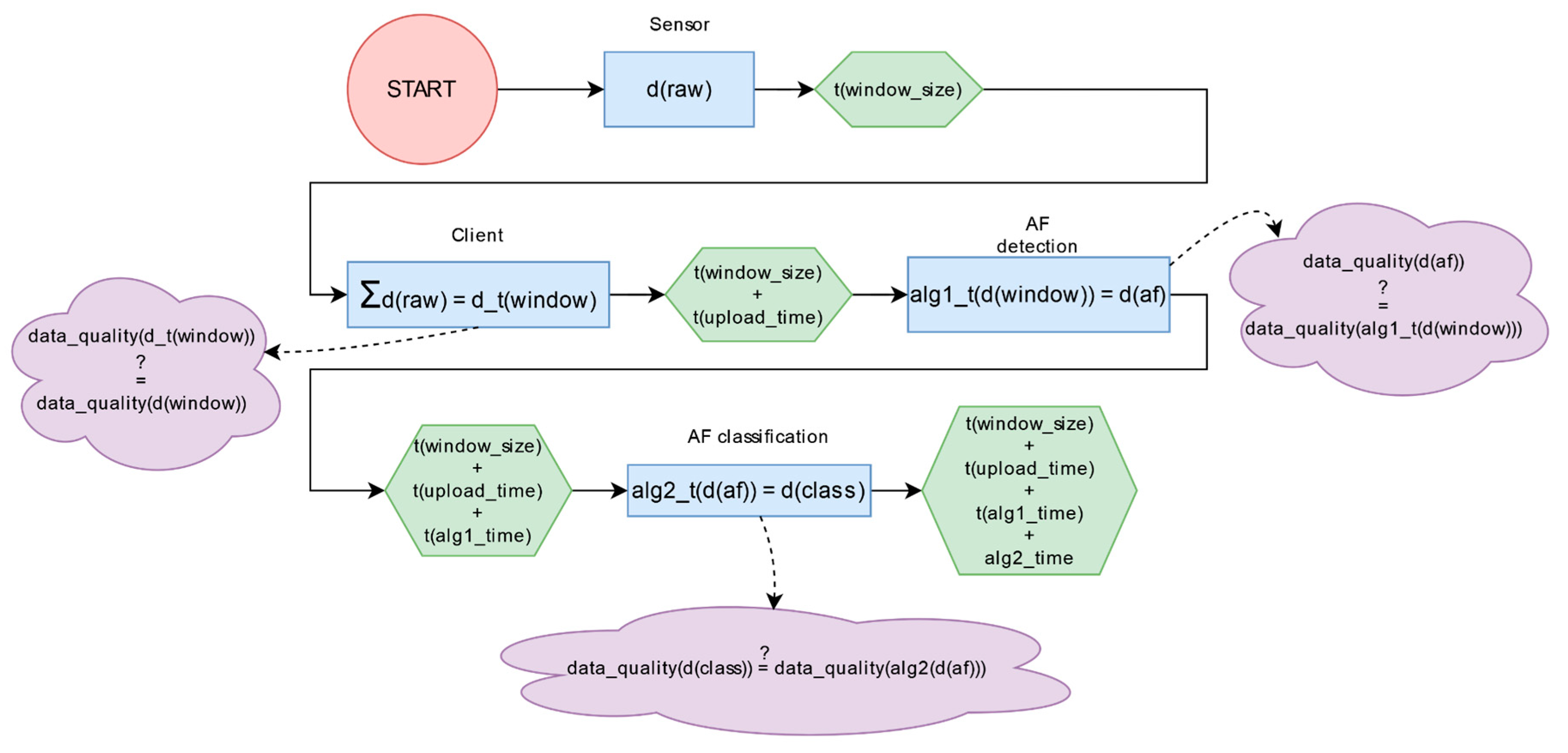
Figure 5 presents the transformation applied on the data and functions that affect the results. $d\left(raw\right)$ represents the raw ECG data obtained from the IoT sensor. After a defined time, the collected raw data form a data window. Here we can measure data quality if needed but in our offline case the data is available. The data window is sent to the AF detection algorithm that produces the output as to whether AF is detected and how long the episode is. Here, a data quality measurement can be performed because some windows may be lost. The $d\left(af\right)$ results can be forwarded to the classification algorithm, where a new data quality measurement can be performed after a possible deterioration in the quality of the input data.

A dropped data window can significantly degrade data quality but may have more severe consequences following an additional aggregation step. This is crucial in real-time systems, especially when it affects human lives. Based on this phenomenon, we consider it important to analyze how such a system works and how data quality changes when some of the data parts are lost.

Using the conditions presented in Equations (1)–(4), we have implemented the model in TLA+. The formal definition of the system can be seen here.

In this formal specification, we defined 3 constant values. MAX_NUM_WIN acts as a termination condition that describes the length of the measurement process, which tells us how many data windows we can have. If we did not set this up, the model checker would never stop. WINDOW_SIZE stands for the length of the window in time. TIMEOUT_UP is the configured timeout value of the upload process. numWin, now₁, now₂, now₃, now₄, dropList, u_i, p_i1 and p_i2 are the variables that we check after every step. numWin is the main counter of the system and it is always compared to MAX_NUM_WIN. now_i contains the current time value in the ith process. dropList is the tuple of the dropped and undropped windows. It contains only Boolean values, TRUE if the window has to be dropped, and FALSE if it can be processed. The latencies of the upload process and the algorithms are assigned to the u_i, p_i1 and p_i2 variables, respectively. UPLOAD_LATENCY, PROC_TIME_ALG_1 and PROC_TIME_ALG_2 are input variables that take values from predefined intervals.

3.5. Model Verification

After constructing a system model in TLA+, it can be easily evaluated using TLC. In fact, TLC acts as a simulation tool that creates a graph in which the nodes represent the states and the edges represent the processes. This modeling and simulation method is more efficient than other simulation techniques, such as Monte Carlo simulation [26], because the entire state space can be evaluated in a short time and states that occur very rarely can also be examined. The results can be compared to the known best and worst-cases and an average and a standard deviation can also be calculated for the data quality. Before starting the model checker, we have to assign values to the defined constants. As is written in a former study [27], by increasing the number of variables in a system, the size of the system grows exponentially, which is called the “state explosion problem”. However, the size of the state space can be limited by using or defining input variables with fixed values or intervals. Before starting the model checking and assigning an infinite set of numbers to the variables and huge values to the constants, we have made a prior calculation in order to estimate the complexity of the problem.

Table 1. Size of state space considering the length of the observed measurement period.

Examined Time Period	Maximum Number of Windows	Number of Possible Outcomes after One Step	Number of Possible States
10 s	1	2	$1$
30 s	3	2	$4$
1 min	6	2	$32$
5 min	30	2	$536,870,912$
10 min	60	2	$5.7646\times {10}^{17}$
30 min	180	2	$7.6625\times {10}^{53}$
1 h	360	2	$1.1743\times {10}^{108}$
3 h	1080	2	$2^{1079}$
6 h	2160	2	$2^{2159}$
12 h	4320	2	$2^{4319}$
24 h	8640	2	$2^{8639}$

concludes the number of possible outcomes that would be verified using different values for total number of windows. The maximum number of windows defines when the model checker has to terminate. If we have 10 s long windows and the maximum number of windows is set to 1, we can only have $2^{1-1}=1$ states, because the first window cannot be dropped because of latency. However, it is not true for the further states, so every other state can have two possible outcomes. All in all, it can be said that the number of possible states of the system can be calculated with the formula in Equation (5).

$$2^{W-1} , where W\in {\mathbb{Z}}^{+}$$

(5)

If we were to evaluate a 24-h simulation within 1 s, it would take years to evaluate the entire state space. However, the problem is not as simple as it seems to be. The number of possible states would be much more if we tested the system with all possible latency values.

We added three input variables, UPLOAD_LATENCY, PROC_TIME_ALG_1 and PROC_TIME_ALG_2. In order to limit the size of state space, we assign intervals to the input variables, so the model checker evaluates the model with all possible values from the intervals and we can still have a wide and focused state space that describes our system well. However, we still have to deal with the number of data windows because an ECG holter is usually worn for at least 24 h. On the one hand, the window size can be increased in order to have fewer data windows in a 24-h measurement, but the window size must be kept within reasonable limits to have interpretable data and not lose the real-time capability of the system. On the other hand, if we just simply terminate the simulation after a given number of evaluations, we cannot guarantee that our results are representative. In order to have accurate results for the data quality, we try to move the model parameters as close to reality as possible. If we use random values, we cannot be more accurate than a Monte Carlo simulation or a random test. All the three input variables can be approximated well if we know their behavior in the system. Based on their roles, we try to assign values from their distribution. If we assign values to the input variables from a distribution that describes the probability variable well, the simulations can also be informative after a small number of executions. Next, we present a methodology to find an accurate PDF based on real executions.

3.6. Finding the Distribution of Input Variables

Here, we have to assign values to three different input variables: UPLOAD_LATENCY, PROC_TIME_ALG_1, PROC_TIME_ALG_2. UPLOAD_LATENCY stands for the time needed to transfer the raw ECG data between the client and the server. Since the upload time can be represented as a Transmission Control Protocol (TCP) traffic flow, we can use a probability distribution that is commonly used for latencies in network traffic. In computer networks, taking into account the capabilities of TCP, it is obvious that small packets are more likely to occur in a TCP session than large packets, due to the Maximum Transmission Unit (MTU) [28]. This concept can significantly improve the latency in a network. Since there are more small packets in the session, the packet size follows a long-tailed distribution. Arfee et al. [29] highlighted the role of the Weibull distribution in Internet traffic modeling. Based on all observations [30], we applied the Weibull probability distribution to provide an accurate approximation of the upload time value. A basic upload time is the ratio of the payload of the packet to the guaranteed bandwidth of the upload.

PROC_TIME_ALG_1 and PROC_TIME_ALG_2 variables denote the execution time of the aggregation algorithms. Since the execution time of a third-party algorithm depends heavily on the applied programming techniques, the input data and the amount of resources allocated to the execution, determining the probability distribution is a more complicated task. Here, we gathered samples from the algorithm execution. We started with the AF detection algorithm that processes the raw ECG data window and returns back if, and how often, it detects AF. In order to obtain homogeneous execution times, we need to make sure that the following two conditions are met.

• Since execution times can vary greatly between systems, it is important to evaluate the algorithm on the same system.
• A significant number and a variety of input data is used during evaluation.

Considering the use case, the algorithms are running in the cloud, so we wanted to have a simulation environment that can be easily used in different environments. We use a portable environment in the form of a Docker image [31], so we can start container instances, running the algorithm with pre-configured resource limits. This is also reasonable because different computing instance configurations can be started with different costs. In order to fulfill the second requirement and have a representative data set, we used the training and validation set of CinC Challenge 2017 [20,21]. We created a histogram of the execution times and tried to find the best matching PDF using the Python package Scipy [32]. The best matching function must have the lowest Sum of Squares for Error (SSE) that is calculated with the formula presented in Equation (6) [33].

$$SSE={{\displaystyle \sum }}_{i=1}^n{(Y{\prime }_i-Y_i)}^2$$

(6)

Although the best-fit PDF produces the lowest SSE, this value can be further reduced by fine-tuning the parameters of the function. Our goal is to find the distribution that best describes reality.

This is the point when we turn to a global optimization problem. There are several methods for finding the global optimum. We tested all Genetic Algorithm (GA), Particle Swarm Optimization (PSO) and Simulated Annealing (SA) techniques but, as it found in many studies [34,35], PSO produces the most accurate results in parameter finding. Our framework supports all three methods, so users can choose which one to use, but PSO is set to default. After finding the optimal parameters of the PDF, we can generate samples from the distribution and the samples can be assigned to the input variables in the model. The above explained methodology can be applied to the second algorithm as well except for the database extension, because its input is the output of the first algorithm.

3.7. Simulation and Evaluation

After initializing the constants and the input variables, a simulation can be started. The more simulations are performed, the more accurate data quality results can be obtained. Since the input variables are given values according to a distribution function, a specific simulation is described with a TLA file, so that each model file contains the values assigned to the input variables. TLC verifies the generated model files using a predefined configuration file. The simulation result is an ordered list of Boolean values indicating whether the given window in the sequence should be dropped or not. From the simulation, it can be seen how many windows of data are dropped. The data quality values can be retrieved by executing the original algorithm implementation and using the output of the simulation as input.

4. Results

The methods used by our framework were presented in Section 3. Now, we show how our framework performs and what results it yields when applied to our use case.

4.1. Identical Runtime Environment

To retrieve the execution time of the algorithms, we created an identical environment. First, we tested the algorithm running in the cloud with different configurations.

Table 2. Average execution time of AF detection algorithm using different computer configurations.

Configuration	Average Algorithm Execution Time per Windows
CPU: 200 MHz Memory: 128 MB	>10 s
CPU: 400 MHz Memory: 256 MB	~10 s
CPU: 800 MHz Memory: 512 MB	~5 s
CPU: 1.4 GHz Memory: 1024 MB	~2 s
CPU: 2.8 GHz Memory: 2048 MB	~1 s
CPU: 4.8 GHz Memory: 2048 MB	~1 s
CPU: 4.8 GHz Memory: 4096 MB	~1 s

lists the available configurations in Google Cloud [36] for a cloud function instance.

After testing the AF detection algorithm in the cloud, we found that the AI model running on low-end Central Processing Unit (CPU) configuration needs more than 10 s to analyze a 30 s long ECG data with one lead. Naturally, increasing the CPU master clock signal can notably decrease the execution time. Using a high-end configuration, the execution time can be reduced below 1 s. However, the prices of the different configurations may vary greatly, so this can also be a viewpoint.

In order to have such an environment that is portable and can be fine-tuned, we instantiated Docker containers with the same amount of resources. CPU usage is limited to one thread, and always the first thread can be used. Maximum allocated memory is 256 MB. This setting was tested on three different computers and servers. The available resources were the following:

• Intel(R) Core(TM) i7-8700K CPU @ 3.70 GHz (6 cores), 32 GB RAM
• Intel(R) Core(TM) i7-11700K CPU @ 3.60 GHz (8 cores), 32 GB RAM
• Intel(R) Xeon(R) E5-2660 CPU @ 2.20 GHz (8 cores), 128 GB RAM

After evaluating the execution times, we found that the CPU usage limit must be fine-tuned slightly based on the used bare metal, but we can create identical environments.

4.2. Fitting Distribution to the Upload Time

In order to give an approximation to the upload time, we used two techniques, service rate and a distribution function. Service rate can be calculated as the ratio of the available link capacity and the average packet size [37]. This provides an average service rate but the exact values always change. In order to add more space to the upload time, we introduced a distribution function that describes network traffic well. In a recent study [29], it was proved that the Weibull distribution can accurately describe inter-arrival time and it is also found which parameter values can be used for adding features of a given network type. In the PDF of the Weibull distribution, the most important parameter is the shape parameter (k). In case of ISP Core Network traffic, k can be set to 0.9. This is the highest possible shape value if we consider network packets. If a DSL or Ethernet Access Networks are available, the k parameter should be lower, about 0.81. Wireless Hotspot Access Networks can be simulated with the lowest k value (0.75). The scale parameter (λ) can be approximated based on the Superposition theorem [38]. Superposition theorem states that in any linear, bilateral network in which multiple sources can be found, the resulting response is the sum of the responses from each source separately. Mitov showed that this superposition converges asymptotically to the inter-arrival process with Weibull distribution [39]. Based on that research, the rules listed in Equations (7) and (8) are valid.

$$k\to 1-\alpha$$

(7)

$$\lambda \to C\sin \frac{\pi \alpha }{\pi \left(1-\alpha \right)}, where 0<C<\infty$$

(8)

Since the shape parameter is well-defined for the different types of networks, the scale parameter can be calculated using the correlations. In Figure 6 it is clearly visible how different network types determine the shape and scale parameters. We calculated the mean of the distributions in order to see the expected value for inter-arrival time in seconds. If the average inter-arrival time is calculated from the bandwidth and the average packet size, the shape and scale parameters can be further tuned. In our use case, a mobile device is used to transfer data, so the shape parameter was set to 0.75.

4.3. Fitting Distribution to the Dataset

To obtain a representative sample of execution times, we needed diverse inputs. We used the CinC 2017 training and validation sets, so we had 8828 ECG recordings. We constructed a histogram of the execution times with a 0.001 precision that is also presented in Figure 7.

The histogram shows a Gaussian-like distribution of execution times, but there is also a long-tail end. An interesting fact is that there is also a small bell curve at the beginning of the histogram. In order to explain these phenomena, we have dived into the dataset and analyzed it from different perspectives. We found that the database contains data windows in which some records are missing or contain 0 values. This may happen because of sensor failures or due to connection issues between the sender and the receiver. If too much data is missing, a smaller window section must be dropped. In such cases, the start and end time of the window does not change, but there are fewer records to be processed, so the execution time is shortened. In addition, when the algorithm reaches the end of the measurement data series, shorter data windows can be found, so the algorithm can return results much more quickly. A detailed analysis can be seen in Figure 8. Axis-X displays the execution time in seconds with a precision of 0.001, whereas axis-y shows the number of ECG signal data for which a given execution time was recorded. To enable straightforward comprehension of the phenomenon, we utilized a subset of the entire dataset containing windows with and without AF as well as windows with less valuable records. ECG data in which AF is detected are colored with a yellow-red gradient, whereas ECG data without AF signals are colored with a white-black gradient. The precise color of a point is determined by the number of dropped window components. The size of the points indicates the number of AFs detected in the ECG data. It is observed that both the number of deleted window components and the number of AF signs can have a significant impact on the execution duration. The long-tail feature of the distribution is primarily caused by ECG data containing AFs; therefore, if an ECG window contains an AF, it requires more time to be processed. The execution time is shorter if the ECG signal is shortened due to missing windows, as indicated by the black and red points. The minor bell curve at the start of the histogram is caused primarily by the corrupt data windows.

An accurate histogram is the basis of finding the fitting PDF. Initially, the form of the histogram looks like a Gaussian-like PDF, so we wanted to make sure if it is a Gaussian distribution or not.

We implemented a component that is now an important part of our framework that uses a selected approximation method to find the best parameters of a given PDF that may fit the shape of the histogram. Here, we used the Gaussian PDF as a basis that is presented in Equation (9).

$$\frac{1}{\sigma \sqrt{2\pi }}{e}^{-\frac{1}{2}{\left(\frac{x-\mu }{\sigma }\right)}^2}, where \mu \in ℝ and {\sigma }^2\in {ℝ}_{>0}$$

(9)

The bell curve is determined by two parameters, μ and σ. μ defines the position of the peak of the curve on the axis-X and must be a real number, and σ controls the width of the curve and must be a positive real number. It is important that the PDFs can have values ranging from 0 to 1. Since our histogram is not in this range, we have to normalize our results first and then assign probability values to the bins. After comparing the effectiveness of global optimization methods, PSO was set as default. Unfortunately, PSO did not find a fitting PDF, but in order to ensure that the algorithm works properly, we proved that the distribution is not Gaussian by using tests. For validation purposes, we elaborated a testing environment for verifying the distribution results. There are various tests available to check if a sample conforms to a given distribution. In our study, we used six different techniques to test our null hypothesis. The null hypothesis is that X comes from Gaussian distribution. The results of the tests are presented in

Table 3. Results of null hypothesis tests for Gaussian distribution.

Test	Result
D’Agostino K2 test	rejected
Shapiro-Wilk test	rejected
Anderson-Darling test	rejected
CHI2 test	not rejected
Jarque-Bera test	rejected
Kolmogrov-Smirnov test	rejected

. We see that 5 out of 6 tests rejected the null hypothesis, so now we can say with confidence that the distribution is not Gaussian.

Based on the results, we needed to find another distribution that describes more accurately the execution times. We used the scipy package in Python that has more than 100 different distributions implemented. After testing every distribution by fitting a curve to our histogram with the lowest SSE, we kept the five best results and found that the Johnson’s SU distribution [40] produced a relatively low SSE (111.51). Its PDF can be seen in Equation (10).

$$\frac{\delta }{\lambda \sqrt{2\pi }}\frac{1}{\sqrt{1+{\left(\frac{x-\xi }{\lambda }\right)}^2}}{e}^{-\frac{1}{2}{\left(\gamma +\delta {\sinh }^{-1}\left(\frac{x-\xi }{\lambda }\right)\right)}^2}, where \gamma ,\xi \in ℝ and \delta , \lambda \in {ℝ}^{+}$$

(10)

To validate whether it describes our execution time histogram more accurately than the Gaussian PDF, we executed the GA, PSO and SA algorithms again to find the best parameter values producing the lowest possible SSE. The Johnson’s SU PDF has four parameters as follows:

• γ controls the flattening of the tail and it must be a real number: if γ > 0 then it flattens the left tail, if γ < 0, it flattens the right tail
• δ adjusts the width and it must be a positive real number: the smaller δ, the wider the function
• ξ sets the position of the function on axis-X and it must be a real number: if ξ > 0, then the function is moved to a more positive domain, if ξ < 0, then the function is moved to a more negative domain
• λ controls the apex and and it must be a positive real number: if λ is higher, then the apex is moved to the positive domain, if λ is lower, then the apex is moved to the negative direction

In

Table 4. Comparison of approximation methods in finding the best parameters for Johnson’s S_U distribution.

Approximation Method	Parameters	SSE
GA	γ = −0.44013026 δ = 32.52262997 ξ = 0.31010099 λ = 0.17227367	15.4543
PSO	γ = −0.43741796 δ = 30.0 ξ = 0.31001392 λ = 0.16483363	15.4407
SA	γ = −1.23205541 δ = 109.67317707 ξ = 143.09754355 λ = 771.84080061	53.9464

, we collected the results of the algorithms. GA found four parameters with 15.4543 SSE, PSO produced moderately different parameters with lower 15.4407 SSE and unfortunately SA worked with an outlier 53.9464 SSE that is definitely the worst result. The results were drawn back to the original histogram and it is seen that the Johnson’s SU PDF approximates slightly better the long-tail feature. Figure 9 depicts the histogram and the calculated PDFs.

Using the distribution functions, we generated random samples for the execution time of the first algorithm. In the case of the second algorithm, the idea is identical with that presented here. The histogram can be seen in Figure 10.

4.4. Data Quality Results

After finding the correct distributions of the latency values, we generated the TLA specifications of 10,000 instances. As a result, TLC collected the list of windows and the information as to whether they were dropped or not due to latency, and this list was saved into a file. The file content is a sequence of windows with statuses in the form of Boolean values. This sequence is applied to real executions using the pretrained AI model and the ECG dataset, so AI processes only those windows of the ECG dataset that have not been dropped due to latency. After evaluating the executions, we split the results into two sets. We measured the data quality and collected the anomalies after both the first level of aggregation and the second level of aggregation. At the first aggregation level, data quality loss is determined by the average number of AF episodes and AF windows missed in the simulations. At the second aggregation level, data quality loss shows the proportion of misclassifications in the breakdown of the chosen classification algorithms.

Table 5. Data quality losses after dropping data windows.

Use Case	Data Quality Loss in Simulation-Based Dropping	Data Quality Loss If Every Second Window Is Dropped
Average number of AF episodes	2.5%	1.75%
Average number of AF windows	4.25%	14.5%
Classification #1	12.99%	22.07%
Classification #2	20.78%	14.29%
Classification #3	12.74%	16.87%
Classification #4	12.85%	17.12%

presents the summary of our results.

It is seen that, on average, we dropped 15.11% of the windows due to latency in this use case and the average of detected AF windows reduced by 4.25%. AF episodes showed a different decrease of only 2.5%. We found it interesting to see how data quality decreases if we dropped every second window. It was observed that the number of AF windows were reduced by 14.5%, but the number of AF episodes became higher than in our simulation. This is because fewer windows are far apart in time and cannot be considered connected.

5. Discussion

After diving deep into the results, we found that the dropped windows can restructure the AF cases and it is also possible that many new short AF periods are generated from a long AF period, so it is important not to make decisions on corrupted data, but to add additional heuristics to data processing. We also took an overview on AF episode durations and inspected how minimum and maximum lengths of AF episode changes after dropping valuable windows. In the most outlier scenario, the maximum duration of an AF episode was dropped from 22 min 19 s 294 ms to 3 min 31 s 125 ms. It means that more than a 20 min long episode is fully lost. In the same scenario, if every second window is dropped, only a 3 min 786 ms long episode is kept. Considering the minimum AF durations and due to the dropped windows, we can have very short, so-called micro AFs. The minimum duration is always under 1 s after dropping windows. In the original data, we did not find AFs shorter than 1 s. The average AF duration can also drastically change. The most outlier case was a decrease from 542 s to 131 s.

Finally, we added the second level of aggregation to the data with reduced data quality. We tested the AF classification system with multiple algorithms. It was observed that the main issue is the number of lost episodes and this is valid for the long ones, but in many cases the number of short episodes started to rise. The final classification changed in many cases. Since the classification algorithms are not as sensitive as the AF detection algorithm, outstanding changes can be seen only in the first aggregation level. If the output of the classification changes, it may lead to wrong therapy or an increased risk of stroke. The first classification algorithm is the most common, which distinguishes four classes, first detected, paroxysmal, persistent and permanent [21]. Here, our ECG records are not longer than 24 h, so the persistent and permanent classes cannot be authoritative considering the data. Nevertheless, first detected and paroxysmal classes can be measured in binary interpretation. After evaluating the simulations, we found no data quality reduction.

The second classification algorithm [22] has five classes, considering the length of the AF episodes. Here, we have AF episodes that last longer than 24 h, episodes which are at least 6 h but at most 24 h long, AF episodes from 1 to 6 h, periods between 10 min and 1 h and intervals shorter than 10 min. According to the classification method, AF episodes shorter than 10 min are not considered as real AF episodes. In our database, we did not have AF episodes longer than 6 h. It was observed during our simulation that there were no missed AF episodes between 1 and 6 h length, but we can see a decrease in the last class.

Later, we evaluated the results using the third classification algorithm [22] that has two classes but here, the recurrence rate is more important than the length. If the number of AF episodes are at least five, ECG data receives a 5+ label, if it is less than five, the recurrence is not relevant. It is observed that during our simulation, we lost some AF episodes, so there is more than 15% reduction in the data quality.

The fourth algorithm [23] classifies the ECG data based on the duration of AF episodes, but now the subclinical AF episodes are taken into account. Four classes are distinguished: AF episodes longer than 5.5 h, episodes between 20 s and 5.5 h, periods between 15 and 20 s and AF intervals shorter than 15 s. Although there was no data in the first and third classes, 12.74% data quality loss was measured.

Finally, the last classification algorithm [24] predicts based on the AF episode length. We can differentiate episodes shorter than 20 s and longer than 20 s. The classes refer here to risk of stroke. Again, the data quality is reduced by 10% in the simulation. Here, we can see the issue of fragmentation in case of dropping every second window. The classifier found two times more short AF episodes.

Overall, the results demonstrate that latency can have an effect on data quality. It was stated in [15] that data quality decline can have significant effects on decisions. To avoid errors, it is recommended to choose the secure option when data quality is poor. It is additionally shown that this framework can be used to simulate such environments and systems in order to observe how varying the latency affects the data quality.

6. Conclusions

In this paper, a hybrid framework capable of modeling and evaluating data quality in real-time telemedicine systems is presented. Alongside a system specification, we have provided a use case that demonstrates how our simulation and emulation techniques can be applied to various system components. Using simulations, we are able to observe how data quality changes under specific conditions. Our simulations are capable of closely approximating the operations of the algorithms, allowing correct results to be obtained even with a comparatively limited database. After analyzing our results and multiple classification algorithms, it was determined that latency can have a substantial impact on data quality, to the point where the reduction can exceed 15%. Future plans include benchmarking our hybrid approach and applying it to other types of real-time systems. Furthermore, we plan to integrate machine learning into this framework so that data quality can be predicted without the need for simulations. Large Language Models (LLM) make it simple to comprehend processes and algorithms, and they can extend our framework with an asymptotic analysis based on the implementation of the algorithms and the data structures used.