Abstract
Deep lifelong learning models can learn new information continuously while minimizing the impact on previously acquired knowledge, and thus adapt to changing data. However, existing optimization approaches for deep lifelong learning cannot simultaneously satisfy the following conditions: unrestricted learning of new data, no use of old data, and no increase in model parameters. To address this problem, a deep lifelong learning optimization algorithm based on dense region fusion (DLLO-DRF) is proposed. This algorithm first obtains models for each stage of lifelong learning, and divides the model parameters for each stage into multiple regions based on the parameter values. Then, based on the dispersion of the parameter distribution, dense regions are dynamically obtained from the divided regions, and the parameters of the dense regions are averaged and fused to optimize the model. Finally, extensive experiments are conducted on the self-labeled transmission line defect dataset, and the results show that DLLO-DRF has the best performance among various comparative algorithms.
1. Introduction
Deep lifelong learning has gained significant attention in recent years [1,2,3]. It requires multiple stages and iterations, and generates multiple corresponding models in each stage. These models at different stages contain varying depths of knowledge. Utilizing this knowledge in an integrated manner can enhance lifelong learning model performance. However, since lifelong learning involves continuously acquiring data, it is impractical for all data to be obtained in a single training session. Moreover, in different training stages, the previously acquired knowledge is affected due to the random update of parameters, which subsequently leads to the decrease in the overall performance of the lifelong learning model.
Another factor leading to lower performance of the model is the sense of fragmentation introduced during the staged training of deep lifelong learning. This fragmentation hampers the overall parameter update process and prevents the trained model from reaching its optimal performance, even when using the same final dataset. Therefore, addressing these challenges remains a focus of current research on deep lifelong learning.
Currently, research on deep lifelong learning has focused on optimizing neural networks through three main approaches. The first approach involves restraining the number and magnitude of neuron parameter updates by introducing various regularization terms into the loss function. For example, the classic EWC [4] method penalizes changes to important parameters in subsequent task training through elastic weight merging. LwF [5], LFL [6], and DMC [7] use the output of the previous model as a soft label for the previous task to reduce forgetting and knowledge transfer. The second approach aims to enable neural networks to review previously learned knowledge through data replay. This is achieved by employing a standard first-in-first-out (FIFO) buffer and selectively storing old knowledge in long-term memory. The third approach involves expanding the network’s capacity to retain more knowledge. This can be accomplished by employing redundant parameters in large deep networks, allowing them to accommodate the learning of new tasks while preserving previously acquired knowledge.
These above approaches offer the advantage of not requiring explicit consideration of previously trained models when new data arrives. However, these approaches also present several challenges. Firstly, they often entail imposing restrictions on the learning of new data during model training. Secondly, they rely on using old data to “review” the model, which can be cumbersome. Lastly, expanding the model’s parameter count to retain more knowledge may lead to increased complexity. Inspired by the theory of model integration technology, we propose an optimization method for deep lifelong learning based on dense region fusion (DLLO-DRF). This method aims to enhance the performance of the final lifelong learning model by effectively integrating the model parameters from each stage of lifelong learning [8,9,10]. By searching for model weight parameters that possess the capability to express data at all stages of lifelong learning, we can achieve significant improvements in the performance of lifelong learning models.
This paper makes the following key contributions:
- A deep lifelong learning optimization method, DLLO-DRF, is proposed, and its corresponding objective function is designed. This method analyzes the differences in the distribution of model parameters in different stages of lifelong learning, and then dynamically integrates these model parameters to obtain weight parameters that effectively capture the overall data patterns.
- Dense region fusion is introduced into the objective function of DLLO-DRF, and the corresponding algorithm is designed.
- Comparative experiments are conducted using self-labeled transmission line defect datasets, and with various deep object detection algorithms. The results show that DLLO-DRF effectively improves the performance of deep neural network models under lifelong learning.
The following sections are organized as follows: Section 2 provides a review of existing works that are relevant to the subject matter discussed in this paper. Section 3 presents the materials and methods in detail, including the objective function and inference process of DLLO-DRF, and experimental material. Section 4 focuses on presenting the obtained results in detail. Finally, Section 5 concludes the paper by summarizing the key findings and discussing the experimental results, as well as drawing overall conclusions based on the research conducted.
2. Related Work
2.1. Deep Lifelong Learning
The concept of lifelong learning [11] was first proposed by Thrun and Mitchell in 1995. In the past few years, the rapid growth and popularity of deep learning has encouraged many researchers to focus on the challenge of continual learning using deep structures [12]. Deep lifelong learning is driven by several key motivations. One is to address the problem of catastrophic forgetting while learning a series of tasks [13], i.e., gradually learn each new task within the same neural network without causing the neural network to forget the model learned from past tasks. The second is how to utilize previously learned knowledge to help better learn new tasks. At present, the optimization methods of deep lifelong learning mainly include methods based on regularization, methods based on knowledge replay, and methods based on parameter isolation.
Based on regularization methods, the regularization term is applied to the loss function to avoid over-updating the parameters of the new model, which in turn prevents the model from forgetting the old knowledge. Lee et al. [14] proposed incremental moment matching, which employs transfer learning techniques such as controlling the posterior parameter search space using L2 norms of old and new parameters to mitigate the forgetting problem. Feng et al. [15] introduced elastic response distillation, an incremental distillation method based on elastic response. This approach focuses on learning the response elastically from the tail class or regression head of the network, evaluating the prediction quality, and selecting valuable responses through elastic response selection strategies. Liu et al. [16] utilized network reparameterization to generate an information matrix based on the previous model training results prior to training a new class in the network. During this training, the gradient direction of parameter updates is adjusted by referencing the information matrix.
Based on knowledge replay, different approaches have been proposed to address the challenge of catastrophic forgetting and leverage previously learned knowledge. Mo Jianwen et al. [17] constructed pseudosamples through a generative model to train them together with new data, effectively constraining the over-updating of parameters and reducing the impact of new data on old knowledge. Isele et al. [18] selectively stored old knowledge in long-term memory using a standard first-in-first-out buffer. They aimed to find the maximum state space coverage by matching data distribution during training, which helps prevent catastrophic forgetting. Inspired by the generation characteristics of the hippocampus as the short-term memory system in the primate brain, Shin et al. [19] proposed a deep generation replay framework. This framework employs a cooperative dual model architecture consisting of a deep generative model and task solutions. By leveraging these two models, the training data of the old task can be easily sampled and effectively fused with the training data of the new task, facilitating knowledge transfer.
Based on parameter isolation methods, Mallya et al. [20] proposed a method to adapt a single deep neural network to multiple tasks without affecting the performance of already-learned tasks, inspired by network quantization and pruning. This method achieves good performance for each task by adding binary masks to the neurons of the original network and assigning different weights to different tasks. Roy et al. [21] proposed an adaptive hierarchical network structure composed of deep convolutional neural networks, which can grow and learn with the emergence of new data. The network grows in a tree-like manner to accommodate new data categories, while also having the ability to distinguish between previously trained categories. Aljundi et al. [22] combined an autoencoder with an expert network to introduce a set of autoencoders for each new task to learn the representation of the current task. During testing, the test samples are automatically forwarded to the relevant expert network.
In addition, there are many lifelong learning optimization methods specific to different application domains of deep neural networks. Chen et al. [23] proposed a meta-learning method that enables the model to adapt to unseen knowledge while overcoming the forgetting problem. This method uses base class samples to train the meta-learner, thus providing better initialization weights, and then fine-tunes the model to mitigate the forgetting problem by retaining the weights associated with the base class. Ramakrishnan et al. [24] proposed a selection mechanism for labeled objects in new classes for the characteristics of two-stage target detection network models. Then, they designed a relationship-guided loss function based on this model, aiming to preserve the relationship of the proposed selection between the base network and the new network trained on other classes. Yan et al. [25] proposed a two-stage learning method that uses dynamically scalable representations for more efficient incremental modeling. The previously learned representation is frozen in each incremental step, and additional feature dimensions of the new feature extractor are used to perform the expansion.
However, existing approaches for deep lifelong learning have some constraints, such as having a greater impact on early tasks, increasing the cost of training, and producing a very large model.
2.2. Deep Model Integration
Deep model integration provides more robust and accurate models by effectively fusing the parameters of multiple models without increasing computational complexity during inference. This makes deep model integration an ideal approach for practical applications that require high accuracy and low inference time. Up to now, there have been two common approaches to obtain the final inference model. One is to train multiple identical models with different training data and then average the weights of the multiple training models. The other is to average the weights of the models over different iterations.
Tarvainen et al. [8] introduced a time-series-based method for averaging model weights that can enhance testing accuracy and utilize fewer labels for training compared to conventional approaches. Huang et al. [26] proposed a technique for fusing multiple neural networks without added training costs by optimizing multiple local minima on the path and employing them as parameters for target neural networks. Izmailov et al. [27] suggested a random weight averaging parameter update approach that offers superior generalization compared to traditional training. Garipov et al. [28] asserted that optimal complex loss function values are connected by simple curves, leading to the development of fast geometric fusion for efficient integrated model training. Frankle et al. [29] analyzed neural networks’ optimization towards linearly connected minimum values under varying data conditions, discovering that stability and prediction accuracy can be improved through random data selection. Matena [9] introduced “Fisher merging,” an alternative merging process utilizing Laplacian approximation that enhances model performance. Von et al. [10] showed improvement in random gradient descent by integrating specific weights and spatially averaging weight space. Wortsman et al. [30] proposed a fine-tuning method that accounts for distribution changes without additional computational costs during the inference stage. Kaddour et al. [31] explored a flat minimum optimizer for training neural networks, merging average and minimax methods to obtain a flatter solution. Neyshabur et al. [32] observed that averaging weight parameters of different instances could share information and improve model robustness and accuracy. In the context of fine-tuning pre-training, Wortsman et al. [33] recommended using the average of multiple model weight fine-tuning events under various hyperparameter configurations, which typically enhances model accuracy and robustness.
The benefits of deep model integration are not limited to improving the overall performance. It can also provide greater model interpretability and help to mitigate the risks associated with model bias or overfitting. Therefore, deep model integration is a promising approach for the future of deep learning.
3. Materials and Methods
3.1. Overall Structure of DLLO-DRF
To address the limitations and challenges associated with various deep lifelong learning algorithms, we introduce DLLO-DRF as a model integration approach. The core concept of DLLO-DRF entails that models generated in each stage of lifelong learning should embody enhanced knowledge concerning the tasks within that stage. For the neural network model, the knowledge is represented by the learned neuron parameters. Thus, by effectively integrating the model parameters from each stage, the overall performance of the deep lifelong learning model can be improved. The complete structure of DLLO-DRF is illustrated in Figure 1.
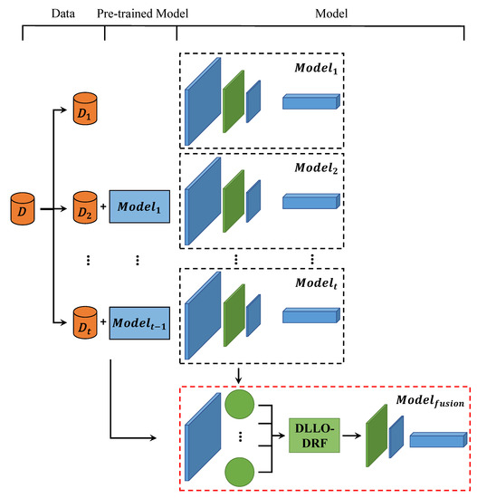
Figure 1.
The structure of DLLO-DRF.
In DLLO-DRF, the dataset is partitioned and trained separately. The first dataset is used for the training of the first stage to obtain Model 1. During each subsequent stage, the dataset for the current stage and the previously trained model are employed to train the present stage’s model. Consequently, DLLO-DRF effectively derives trained models from multiple stages. Then, by selecting and fusing the same network parameter modules from different stages, the fused network parameter modules are obtained. Finally, the fused model is obtained by combining other network modules.
For convenience, important notations are listed in Table 1.

Table 1.
Important notations used in this paper.
3.2. Algorithm Principle in DLLO-DRF
DLLO-DRF integrates parameters that are obtained from multiple stages of lifelong learning. The algorithm consists of two parts. The first part is the obtaining of models for each stage of lifelong learning, and the second part is the dense region fusion on the network model parameters. This section provides a detailed introduction to these two parts separately.
3.2.1. Lifelong Learning Paradigm Based on Model Fine-Tuning
A lifelong learning algorithm that is based on the model fine-tuning approach requires the condition that when new information is learned, only previous knowledge is tuned, instead of relearning all the information. This can significantly reduce computational complexity and allow the model to learn new information faster. The fine-tuning approach can take full advantage of the powerful generalization capabilities of deep learning neural networks, and can avoid the need to design new models and train from the beginning, converging faster and with better results. This offers many advantages, such as the model having a high initial performance before training, gaining faster improvement of the model during training, and having better convergence than the obtained model. This lifelong learning paradigm is universal, and it can be applied to all deep learning algorithms. The models trained through this paradigm also provide support for fusion. The lifelong learning paradigm based on model fine-tuning can be summarized as using data from the current stage of lifelong learning tasks, and using the task model of the previous stage as a pre-training model to train the task model of the current stage. The following paragraph provides a definition of the model-fine-tuning-based lifelong learning paradigm.
The initial training dataset, noted as D, is divided into n parts: . The training dataset used in the stage in lifelong learning is defined as . represents the model obtained by employing training dataset A to train pre-trained model B using algorithm . represents the model obtained in the stage, and is defined as follows:
where represents other pre-trained models that can be selected in the first stage.
3.2.2. Dense Region Fusion
In order to observe the distribution of parameters under lifelong learning, we conducted 10 stages of training on the Cascade R-CNN object detection algorithm using the model fine-tuning lifelong learning training paradigm. Figure 2 shows some parameters in the model changing with the task stage, and it can be observed that these parameters are often concentrated in one of the regions. The region with the highest concentration of parameters is referred to as the dense region. For neural networks, these aggregated parameters are more valuable to the model itself, as they often carry the most important knowledge within the model.
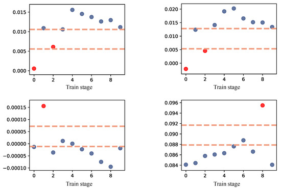
Figure 2.
Fine-tune the distribution of model parameters under lifelong learning. The blue points represent the parameters in the dense region, while the red points refer to those outside the dense region.
Based on the above findings, dense region fusion divides the parameters of models from multiple task stages of lifelong learning into regions at the same location, and takes the average of all parameters in the region with the densest parameter distribution as the parameters of the fusion model. Therefore, the model fused in this way can maximize the information of all stages of lifelong learning tasks. The main steps and related formulas of dense region fusion are introduced in the following paragraphs.
Through the training method defined in Section 3.2.1, we can obtain the model for each stages: . For deep neural network models, the parameter dimensions correspond to the size of the convolutional kernel. Typically, the convolutional kernel size varies across different layers. To enable the fusion process, it is crucial to map the parameter vectors in the network onto a one-dimensional space, as the convolutional kernel size varies across layers. The dimension mapping algorithm is illustrated in Algorithm 1. Through dimension mapping, the parameter at position i of the stage model is represented as . Consequently, the parameter set encompassing all stage models at position i is . In order to identify the most densely distributed region in , it is essential to partition into distinct regions, with each region’s size determined by the parameter range of , computed using Equation (2).
where j is the number of regions that are divided, and and are the maximum and minimum values in , respectively.
| Algorithm 1: Dimension Mapping |
Input: : The set of the trained model. Output: : Model set with weight parameters reduced to one dimension. : Original model parameter dimension. 1 Obtain the parameter dimension in 2 For each model, , traverse all parameters based on their dimensions and merge them into a one-dimensional array; 3 For each model, , replace all the parameters to an array obtained in the last step. |
The region division implementation is depicted in Algorithm 2. Through region division, the j subset of parameter space for all models at position i can be acquired, denoted as . The objective of dense region fusion is to identify the subset with the highest number of parameters within the subsets, namely, the dense region . To circumvent the uncertainty in dense region selection when parameter quantities are relatively evenly distributed across different regions, which could compromise the fusion model’s robustness, the dense region is determined based on . The parameter quantity’s variance is calculated for each subset, and when falls below a predefined threshold, the original parameter set is directly treated as the dense region. The calculation of is carried out using Equation (3).
where represents the number of elements of X, and V is the set threshold of variance.
| Algorithm 2: Region Division |
 |
Finally, the mean value of the parameters in is used as the parameter at the ith position in the fusion model , and it can be calculated using Equation (4).
where represents the number of elements in the set X.
We also offer an approach for directly identifying dense regions. This approach involves constructing a network model that employs short- and long-term neural networks to learn the boundaries of dense regions within a given parameter space, with the model being referred to as a dense region divider. The structure of the region divider is illustrated in Figure 3.
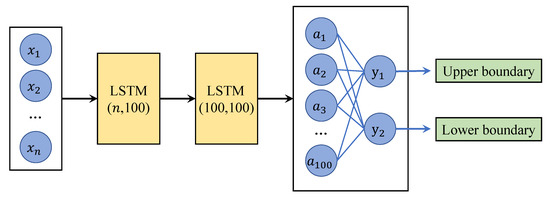
Figure 3.
The structure of the dense region divider network.
The input for the network consists of the parameters of the stage model, followed by a layer of LSTM units with input and output dimensions of . Subsequently, another layer of LSTM units with input and output dimensions of is employed. Finally, a fully connected layer with input and output dimensions of is added. This connected layer’s two outputs represent the upper and lower bounds of the learned dense region. By utilizing this region divider, dense regions can be obtained as an alternative to employing Algorithm 2 and Equation (3).
Based on the principles and steps of the above algorithms, an algorithm for dense region fusion has been developed, which is presented in Algorithm 3.
| Algorithm 3: Dense Region Fusion |
 |
3.2.3. Process of DLLO-DRF
Based on the structure and principles of DLLO-DRF, we give the detailed process of DLLO-DRF in Figure 4. Initially, DLLO-DRF divides the training set and proceeds to train according to the lifelong learning paradigm defined in Section 3.2.1. Subsequently, the parameters of models across all stages are obtained at the overlapping position of the fusion module, followed by the division of these parameters into regions. Finally, the mean value of all parameters within the densest region is utilized as the parameters of the fusion module at the corresponding positions. This step is iterated until all the average values of parameters across every position within the module are fused.
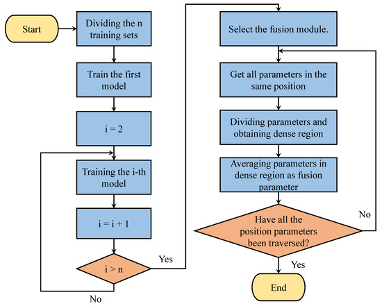
Figure 4.
The process of DLLO-DRF.
3.2.4. Complexity Analysis
In DLLO-DRF, primary variables include m (number of training stages) and n (number of fusion parameters). It contains two components: lifelong learning training and dense region fusion. The time complexity of obtaining parameters and partitioning them is and for a single model, resulting in a total of . Spatial complexity, dependent on model number and size, is also .
3.3. Experimental Material
3.3.1. Dataset
In order to evaluate the performance of DLLO-DRF, a self-labeled transmission line defect detection dataset is utilized, which includes a bird’s nest foreign object dataset, a cement pole damage dataset, an anti-vibration hammer slip dataset, and an insulator self-explosion dataset. These four datasets consist of 385, 384, 385, and 376 images, respectively. Due to the varying degrees and damage methods, defect characteristics may differ within the same defect type, causing uneven data distribution. Figure 5 presents two images from the bird’s nest foreign object dataset, wherein the left image exhibits a bird’s nest and the right one a honeycomb. Despite their distinct types and characteristics, they both pertain to the bird’s nest foreign object category. Lifelong learning training methods are preferable since the model must handle data within the same category but with varying features in the future. Consequently, employing these four datasets in experiments on the proposed algorithm is more persuasive.
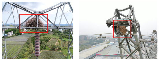
Figure 5.
Example of bird’s nest foreign object dataset image. The defects are marked inside the red box.
The detailed information of the transmission line defect dataset is shown in Table 2.
Table 2.
The detailed information of four defect datasets.
3.3.2. Evaluation Metrics
In the field of object detection, the most commonly used evaluation metrics include Intersection over Union, accuracy, precision, recall, value, value, and value. This section provides a detailed introduction to these evaluation metrics.
Intersection over Union () can be used to determine the degree of overlap between two images. In the field of object detection, the degree of overlap between two boxes can be determined. The calculation of is shown in Equation (5).
where represents the border of the actual object in the image, represents the bounding box predicted by the detection algorithm, and is calculated based on these two values, which can measure the accuracy of the bounding box predicted by the detection model. In object detection, prediction boxes with are generally classified as positive samples, while the rest are classified as negative samples.
Moreover, the correct prediction of positive samples as the number of positive samples is called true (), the correct prediction of negative samples as the number of negative samples is called true negative (), the incorrect prediction of negative samples as the number of positive samples is called false positive (), and the incorrect prediction of positive samples as the number of negative samples is called false negative (). The accuracy, precision, and recall are calculated as follows:
By combining accuracy and recall, a PR curve can be drawn, with recall as the horizontal axis and accuracy as the vertical axis. The larger the area between the PR curve and the axes, the better the performance of the detection model.
The average precision () represents the area enclosed by the PR curve and the coordinate axis, which can be calculated using Equation (9).
is a relatively important evaluation metric, which is generally calculated based on different thresholds for under various thresholds. For example, and represent the measured values of at thresholds of 0.5 and 0.75, respectively. Furthermore, it is possible to calculate all values separately with an step of 0.05 from to , and then take the average value and record it as . This value can fully evaluate the detection effect from more perspectives.
The average recall () is the average of all recalls for from 0.5 to 1.0, and its calculation formula is shown in Equation (10):
The mean average precision () of categories is the average value of s under each category. In the field of object detection, it may be necessary to simultaneously detect multiple categories of objects, and can effectively evaluate the effectiveness of a model in predicting multiple categories of targets. The calculation of is shown in Equation (11).
where K is the number of categories detected, and represents the value under the ith category. If there is only one detection category, then is equal to .
3.3.3. Experimental Setting
The experimental hardware device used a host of the Ubuntu 22.04 LTS operating system, and was equipped with an AMD Ryzen 5600x CPU, NVIDIA TITAN X graphics card, and 64 GB of memory. The software was programmed using Python as the programming language, and Pycharm was used to write the code for the deep learning framework, which was based on Pytorch.
For the settings of the basic algorithm, the datasets used are the four transmission line defect datasets mentioned in Section 3.3.1. The deep neural network model used is the object detection model, which includes three single-stage object detection algorithms, ATSS [34], DDOD [35], and GFL [36], and six two-stage object detection algorithms, which are Cascade R-CNN [37], Faster R-CNN [38], Dynamic R-CNN [39], Grid R-CNN [40], Libra R-CNN [41], and Sparse R-CNN [42]. The feature extraction network adopts a 50-layer residual network ResNet50 [43] and a feature pyramid network FPN. All models have a batch size of 2 and a learning rate of 0.02.
The DLLO-DRF algorithm was set up by dividing the training set into 10 parts and training each algorithm model for 10 stages using the lifelong learning method defined in Section 3.2.1. The FPN module parameters were selected for dense region fusion in the basic algorithm, with a region division number of 3 and a variance threshold of 2.
Furthermore, , , , and were selected as the evaluation metrics. The metric is consistent with the one used in the COCO dataset [44], which refers to , as mentioned in the summary.
3.3.4. Friedman Test
The first step of the Friedman test method involves sorting the algorithm performance from good to poor based on the evaluation metrics in each dataset, and assigning order values of 1, 2, 3, etc. If the algorithm performance is the same, the order values are divided equally. Once the order values for each algorithm have been assigned, the average order value is calculated across all datasets. The second step involves calculating the test statistics required for the test, according to Equations (12) and (13).
where k represents the number of algorithms, N represents the number of datasets, is the average order value of the algorithm, and the final calculated follows the F distribution with degrees of freedom of and .
The significance is often set to 0.05 in hypothesis testing. The original assumption is that there is no significant difference in the performance of each algorithm. When the calculated is greater than , the original assumption is accepted, that is, there is no significant difference in the performance of each algorithm. When the calculated is less than , the original assumption is rejected, meaning that there are significant differences in the performance of each algorithm.
4. Results and Analysis
4.1. Experiment Effect of Lifelong Learning Training
For datasets with small differences in data distribution, a good lifelong learning model can make the model better, as more data becomes available. For optimization algorithms, a good lifetime learning pattern can also provide more effective information for subsequent fusions. To verify the effectiveness of the lifetime learning approach for the defective dataset mentioned in Section 3.2.1, eight object detection algorithms are selected in this section, and trained on the impact hammer sliding dataset according to the experimental setup described in Section 3.3.3. Table 3, Table 4, Table 5 and Table 6 relate to , , , and , respectively. These four metrics demonstrate the performance variation of each algorithm at each stage of lifelong learning.
Table 3.
The index of each algorithm at different training stages under the sliding dataset of the shock hammer.
Table 4.
The index of each algorithm at different training stages under the sliding dataset of the shock hammer.
Table 5.
The index of each algorithm at different training stages under the sliding dataset of the shock hammer.
Table 6.
The index of each algorithm at different training stages under the sliding dataset of the shock hammer.
The results indicate that the overall performance of the eight object detection algorithms used in the experiment shows an upward trend with the increase in lifelong learning stage across all four metrics. To better illustrate the changes in the model’s overall performance, we plotted line charts for each algorithm’s performance under the four metrics (, , , and ) with the training stage, as shown in Figure 6. The results show that all metrics rapidly increased in the first three stages, and the growth rate slowed down in the last seven stages, while the overall trend remained upward. These observations confirm that the lifelong learning training paradigm defined in Section 3.2.1 can effectively demonstrate the performance of various algorithms on the transmission line defect dataset.
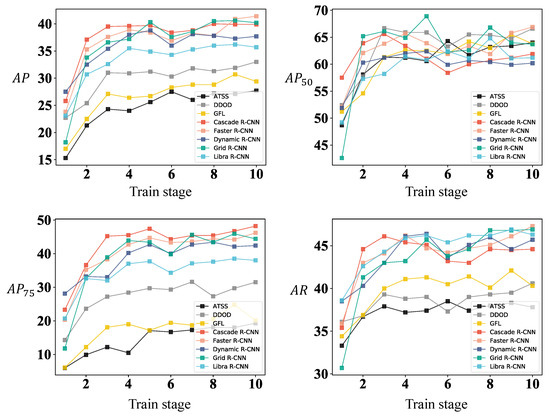
Figure 6.
Trends in metrics of various algorithms in different stages of lifelong learning training.
4.2. Longitudinal Comparative Experiments on Basic Algorithms
4.2.1. Comparison of DLLO-DRF Detection Algorithms Used and Unused in the Bird’s Nest Foreign Object Dataset
Table 7 indicates that using DLLO-DRF improved the average values of the metrics for each algorithm in the bird’s nest foreign object dataset, with improvements observed in , , and .
Table 7.
Comparison of DLLO-DRF algorithms used and unused in the bird’s nest foreign object dataset. The better results are indicated using bold and underline.
4.2.2. Comparison of DLLO-DRF Detection Algorithms Used and Unused in the Cement Pole Damage Dataset
Table 8 shows that using DLLO-DRF improved the average values of the metrics for each algorithm in the cement pole damage dataset, with improvements observed in , , and .
Table 8.
Comparison of DLLO-DRF algorithms used and unused in the cement pole damage dataset. The better results are indicated using bold and underline.
4.2.3. Comparison of DLLO-DRF Detection Algorithms Used and Unused in the Shockproof Hammer Slip Dataset
Table 9 demonstrates that using DLLO-DRF improved the average values of the metrics for each algorithm in the shockproof hammer slip dataset, with improvements observed in , , and .
Table 9.
Comparison of DLLO-DRF algorithms used and unused in the shockproof hammer slip dataset. The better results are indicated using bold and underline.
4.2.4. Comparison of DLLO-DRF Detection Algorithms Used and Unused in the Insulator Self-Explosion Dataset
Table 10 illustrates that using DLLO-DRF improved the average values of the metrics for each algorithm in the insulator self-explosion dataset, with improvements observed in , , , and .
Table 10.
Comparison of DLLO-DRF algorithms used and unused in the insulator self-explosion dataset. The better results are indicated using bold and underline.
4.3. Horizontal Comparison Experiment with Other Algorithms
4.3.1. Comparison between DLLO-DRF and Other Algorithms in the Bird’s Nest Foreign Object Dataset
As shown in Table 11, DLLO-DRF ranks first for three or more metrics among seven detection algorithms. For the metric, DLLO-DRF ranks first among eight detection algorithms. For the metric, DLLO-DRF ranks first among seven detection algorithms. For the metric, DLLO-DRF ranks first among eight detection algorithms. For the metric, DLLO-DRF ranks first among eight detection algorithms. In contrast, for Uniform soup, there is only one algorithm ranking first for the and metrics, and for Greedy soup, there is only one algorithm ranking first for the , , and metrics.
Table 11.
Comparison of DLLO-DRF and other fusion methods in the bird’s nest foreign object dataset. The better results are indicated using bold and underline.
4.3.2. Comparison between DLLO-DRF and Other Algorithms in the Cement Pole Damage Dataset
As shown in Table 12, DLLO-DRF ranks first for three or more metrics among seven detection algorithms. For the metric, DLLO-DRF ranks first among eight detection algorithms. For the metric, DLLO-DRF ranks first among eight detection algorithms. For the metric, DLLO-DRF ranks first among three detection algorithms. For the metric, DLLO-DRF ranks first among eight detection algorithms. In contrast, for Uniform soup, there are two, five, and two algorithms ranking first for the , , and metrics, respectively, and for Greedy soup, there are one and two algorithms ranking first for the , , and metrics, respectively.
Table 12.
Comparison of DLLO-DRF and other fusion methods in the cement pole damage dataset. The better results are indicated using bold and underline.
4.3.3. Comparison between DLLO-DRF and Other Algorithms in the Shockproof Hammer Slip Dataset
As shown in Table 13, DLLO-DRF ranks first for three or more metrics among six detection algorithms. For the metric, DLLO-DRF ranks first among six detection algorithms. For the metric, DLLO-DRF ranks first among nine detection algorithms. For the metric, DLLO-DRF ranks first among five detection algorithms. For the metric, DLLO-DRF ranks first among six detection algorithms. In contrast, for Uniform soup, there is only one algorithm ranking first for the metric, and for Greedy soup, there are three, one, four, and three algorithms ranking first for the , , , and metrics, respectively.
Table 13.
Comparison of DLLO-DRF and other fusion methods in the shockproof hammer slip dataset. The better results are indicated using bold and underline.
4.3.4. Comparison between DLLO-DRF and Other Algorithms in the Insulator Self-Explosion Dataset
As shown in Table 14, DLLO-DRF ranks first for three or more metrics among six detection algorithms. For the metric, DLLO-DRF ranks first among seven detection algorithms. For the metric, DLLO-DRF ranks first among seven detection algorithms. For the metric, DLLO-DRF ranks first among three detection algorithms. For the metric, DLLO-DRF ranks first among seven detection algorithms. In contrast, for Uniform soup, there are one, two, three, and two algorithms ranking first for the , , , and metrics, respectively, and for Greedy soup, there are one, one, and four algorithms ranking first for the , , and metrics, respectively.
Table 14.
Comparison of DLLO-DRF and other fusion methods in the insulator self-explosion dataset. The better results are indicated using bold and underline.
In conclusion, DLLO-DRF outperforms Uniform soup and Greedy soup on all four datasets, and Greedy soup performs better than Uniform soup. The model faces significant parameter update deviations when encountering new data at each training stage under the training conditions based on fine-tuning lifelong learning. DLLO-DRF strikes a balance between fundamental parameters to identify and compute parameters that are appropriate for the entire lifelong learning process, while Uniform soup and Greedy soup integrate all basic parameters, resulting in a weaker expression ability of the integrated model for all data in the entire lifelong learning process. As Greedy soup aims to identify the best metrics, and uses a greedy approach to identify suitable subsets of basic models for fusion, it is more suitable for lifelong learning as a dynamic training method compared to Uniform soup.
4.4. Friedman Test Results
To investigate the differences between the three abovementioned algorithms, the Friedman test method was used to verify the experiment in Section 4.3. Here, the metric is selected for testing all datasets and basic object detection algorithms. The experiment involved three algorithms and used four datasets, and followed the F distribution with degrees of freedom of 2 and 6. According to the distribution, the values for ATSS, DDOD, GFL, Cascade R-CNN, Fast R-CNN, Dynamic R-CNN, Grid R-CNN, Libra R-CNN, and Sparse R-CNN are 0.0293, 0.0293, 0.0293, 0.0421, 0.0293, 0.0293, 0.0293, 0.0293, and 0.0388, respectively, with significance less than 0.05. As a result, we must reject the initial assumption that there is no significant difference in the performance of each algorithm. Therefore, there are significant differences in the performance of the algorithms participating in the experiment. Based on the conclusion of the experiment in Section 4.3, it is concluded that DLLO-DRF has the best performance compared to the comparative algorithms.
5. Conclusions
This paper presents DLLO-DRF, a deep lifelong learning optimization algorithm based on dense region fusion. In this algorithm, the parameters at each stage in lifelong learning are partitioned into regions based on their values. DLLO-DRF identifies dense regions through parameter dispersion analysis, and optimizes the model by averaging and fusing the parameters. In Section 4, extensive experiments on the self-labeled transmission line defect dataset and various deep object detection algorithms demonstrate that the proposed DLLO-DRF effectively improves the performance of deep neural network models under lifelong learning. This significantly contributes to the development of deep lifelong learning by offering an optimization method that simultaneously allows for the learning of new data without using old data, and without increasing the model parameters.
Additionally, as deep lifelong learning is a rapidly growing and evolving field, there are many areas in which DLLO-DRF can be further improved and developed. Further research is required to evaluate the effectiveness of DLLO-DRF on diverse and large-scale datasets. It is also important to explore ways of adapting DLLO-DRF to optimize complex, changing deep neural network models, and make them scalable for large-scale lifelong learning scenarios.
Overall, the proposed DLLO-DRF offers a promising approach for optimizing lifelong learning in deep neural networks, and opens up new avenues for future research and development.
Author Contributions
Conceptualization, L.Z., F.D., S.X. and H.W.; methodology, L.Z., F.D. and S.X.; software, F.D.; validation, Z.C., H.W. and F.D.; formal analysis, L.Z.; investigation, L.Z.; resources, F.D., S.X., Z.C. and H.W.; data curation, L.Z.; writing—original draft preparation, L.Z., F.D., S.X., Z.Q. and Z.C.; writing—review and editing, L.Z., F.D., S.X., Z.Q., Z.C. and H.W.; visualization, L.Z. and F.D.; supervision, Z.C. and H.W.; project administration, H.W. All authors have read and agreed to the published version of the manuscript.
Funding
This research was funded by the Science and Technology Project of the State Grid Sichuan Electric Power Company (grant number 52199722000Y).
Institutional Review Board Statement
Not applicable.
Informed Consent Statement
Not applicable.
Data Availability Statement
Not applicable.
Conflicts of Interest
The authors declare no conflict of interest.
Abbreviations
The following abbreviations are used in this manuscript:
| DLLO-DRF | Deep Lifelong Learning Optimization algorithm based on Dense Region Fusion |
| EWC | Elastic Weight Consolidation |
| LwF | Learning without Forgetting |
| LFL | Less-Forgetting Learning |
| DMC | Deep Model Consolidation |
| R-CNN | Region-based Convolutional Neural Network |
| LSTM | Long Short-Term Memory |
| ATSS | Adaptive Training Sample Selection |
| DDOD | Disentangled Dense Object Detector |
| GFL | Generalized Focal Loss |
| FPN | Feature Pyramid Network |
References
- Zhao, T.; Wang, Z.; Masoomi, A.; Dy, J. Deep bayesian unsupervised lifelong learning. Neural Netw. 2022, 149, 95–106. [Google Scholar] [CrossRef] [PubMed]
- Lee, S.; Stokes, J.; Eaton, E. Learning Shared Knowledge for Deep Lifelong Learning using Deconvolutional Networks. In Proceedings of the IJCAI, Macao, China, 10–16 August 2019; pp. 2837–2844. [Google Scholar]
- Lee, S.; Behpour, S.; Eaton, E. Sharing less is more: Lifelong learning in deep networks with selective layer transfer. In Proceedings of the International Conference on Machine Learning, PMLR. Virtual, 18–24 July 2021; pp. 6065–6075. [Google Scholar]
- Kirkpatrick, J.; Pascanu, R.; Rabinowitz, N.; Veness, J.; Desjardins, G.; Rusu, A.A.; Milan, K.; Quan, J.; Ramalho, T.; Grabska-Barwinska, A.; et al. Overcoming catastrophic forgetting in neural networks. Proc. Natl. Acad. Sci. USA 2017, 114, 3521–3526. [Google Scholar] [CrossRef] [PubMed]
- Li, Z.; Hoiem, D. Learning without forgetting. IEEE Trans. Pattern Anal. Mach. Intell. 2017, 40, 2935–2947. [Google Scholar] [CrossRef] [PubMed]
- Jung, H.; Ju, J.; Jung, M.; Kim, J. Less-forgetting learning in deep neural networks. arXiv 2016, arXiv:1607.00122. [Google Scholar]
- Zhang, J.; Zhang, J.; Ghosh, S.; Li, D.; Tasci, S.; Heck, L.; Zhang, H.; Kuo, C.C.J. Class-incremental learning via deep model consolidation. In Proceedings of the IEEE/CVF Winter Conference on Applications of Computer Vision, Snowmass Village, CO, USA, 1–5 March 2020; pp. 1131–1140. [Google Scholar]
- Tarvainen, A.; Valpola, H. Mean teachers are better role models: Weight-averaged consistency targets improve semi-supervised deep learning results. Adv. Neural Inf. Process. Syst. 2017, 30, 1195–1204. [Google Scholar]
- Matena, M.S.; Raffel, C.A. Merging models with fisher-weighted averaging. Adv. Neural Inf. Process. Syst. 2022, 35, 17703–17716. [Google Scholar]
- Von Oswald, J.; Kobayashi, S.; Sacramento, J.; Meulemans, A.; Henning, C.; Grewe, B.F. Neural networks with late-phase weights. arXiv 2020, arXiv:2007.12927. [Google Scholar]
- Thrun, S.; Mitchell, T.M. Lifelong robot learning. Robot. Auton. Syst. 1995, 15, 25–46. [Google Scholar] [CrossRef]
- Parisi, G.I.; Kemker, R.; Part, J.L.; Kanan, C.; Wermter, S. Continual lifelong learning with neural networks: A review. Neural Netw. 2019, 113, 54–71. [Google Scholar] [CrossRef]
- McCloskey, M.; Cohen, N.J. Catastrophic interference in connectionist networks: The sequential learning problem. In Psychology of Learning and Motivation; Elsevier: Amsterdam, The Netherlands, 1989; Volume 24, pp. 109–165. [Google Scholar]
- Lee, S.W.; Kim, J.H.; Jun, J.; Ha, J.W.; Zhang, B.T. Overcoming catastrophic forgetting by incremental moment matching. Adv. Neural Inf. Process. Syst. 2017, 30, 4655–4665. [Google Scholar]
- Feng, T.; Wang, M.; Yuan, H. Overcoming catastrophic forgetting in incremental object detection via elastic response distillation. In Proceedings of the IEEE/CVF Conference on Computer Vision and Pattern Recognition, New Orleans, LA, USA, 24 June 2022; pp. 9427–9436. [Google Scholar]
- Liu, X.; Masana, M.; Herranz, L.; Van de Weijer, J.; Lopez, A.M.; Bagdanov, A.D. Rotate your networks: Better weight consolidation and less catastrophic forgetting. In Proceedings of the 2018 24th International Conference on Pattern Recognition (ICPR), Beijing, China, 20–24 August 2018; pp. 2262–2268. [Google Scholar]
- Mo, J.; Chen, Y. Class Incremental Learning Based on Variational Pseudosample Generator with Classification Feature Constraints. Control Decis. 2021, 36, 2475–2482. [Google Scholar]
- Isele, D.; Cosgun, A. Selective experience replay for lifelong learning. In Proceedings of the AAAI Conference on Artificial Intelligence, New Orleans, LA, USA, 2–7 February 2018; Volume 32. [Google Scholar]
- Shin, H.; Lee, J.K.; Kim, J.; Kim, J. Continual learning with deep generative replay. Adv. Neural Inf. Process. Syst. 2017, 30, 2994–3003. [Google Scholar]
- Mallya, A.; Davis, D.; Lazebnik, S. Piggyback: Adapting a single network to multiple tasks by learning to mask weights. In Proceedings of the European Conference on Computer Vision (ECCV), Munich, Germany, 8–14 September 2018; pp. 67–82. [Google Scholar]
- Roy, D.; Panda, P.; Roy, K. Tree-CNN: A hierarchical deep convolutional neural network for incremental learning. Neural Netw. 2020, 121, 148–160. [Google Scholar] [CrossRef]
- Aljundi, R.; Chakravarty, P.; Tuytelaars, T. Expert gate: Lifelong learning with a network of experts. In Proceedings of the IEEE Conference on Computer Vision and Pattern Recognition, Honolulu, HI, USA, 21–26 July 2017; pp. 3366–3375. [Google Scholar]
- Cheng, M.; Wang, H.; Long, Y. Meta-learning-based incremental few-shot object detection. IEEE Trans. Circuits Syst. Video Technol. 2021, 32, 2158–2169. [Google Scholar] [CrossRef]
- Ramakrishnan, K.; Panda, R.; Fan, Q.; Henning, J.; Oliva, A.; Feris, R. Relationship matters: Relation guided knowledge transfer for incremental learning of object detectors. In Proceedings of the IEEE/CVF Conference on Computer Vision and Pattern Recognition Workshops, Snowmass Village, CO, USA, 1–5 March 2020; pp. 250–251. [Google Scholar]
- Yan, S.; Xie, J.; He, X. Der: Dynamically expandable representation for class incremental learning. In Proceedings of the IEEE/CVF Conference on Computer Vision and Pattern Recognition, Nashville, TN, USA, 20–25 June 2021; pp. 3014–3023. [Google Scholar]
- Huang, G.; Li, Y.; Pleiss, G.; Liu, Z.; Hopcroft, J.E.; Weinberger, K.Q. Snapshot ensembles: Train 1, get m for free. arXiv 2017, arXiv:1704.00109. [Google Scholar]
- Izmailov, P.; Podoprikhin, D.; Garipov, T.; Vetrov, D.; Wilson, A.G. Averaging weights leads to wider optima and better generalization. arXiv 2018, arXiv:1803.05407. [Google Scholar]
- Garipov, T.; Izmailov, P.; Podoprikhin, D.; Vetrov, D.P.; Wilson, A.G. Loss surfaces, mode connectivity, and fast ensembling of dnns. Adv. Neural Inf. Process. Syst. 2018, 31, 8803–8812. [Google Scholar]
- Frankle, J.; Dziugaite, G.K.; Roy, D.; Carbin, M. Linear mode connectivity and the lottery ticket hypothesis. In Proceedings of the International Conference on Machine Learning, PMLR. Virtual, 13–18 July 2020; pp. 3259–3269. [Google Scholar]
- Wortsman, M.; Ilharco, G.; Kim, J.W.; Li, M.; Kornblith, S.; Roelofs, R.; Lopes, R.G.; Hajishirzi, H.; Farhadi, A.; Namkoong, H.; et al. Robust fine-tuning of zero-shot models. In Proceedings of the IEEE/CVF Conference on Computer Vision and Pattern Recognition, New Orleans, LA, USA, 24 June 2022; pp. 7959–7971. [Google Scholar]
- Kaddour, J.; Liu, L.; Silva, R.; Kusner, M.J. Questions for flat-minima optimization of modern neural networks. arXiv 2022, arXiv:2202.00661v2. [Google Scholar]
- Neyshabur, B.; Sedghi, H.; Zhang, C. What is being transferred in transfer learning? Adv. Neural Inf. Process. Syst. 2020, 33, 512–523. [Google Scholar]
- Wortsman, M.; Ilharco, G.; Gadre, S.Y.; Roelofs, R.; Gontijo-Lopes, R.; Morcos, A.S.; Namkoong, H.; Farhadi, A.; Carmon, Y.; Kornblith, S.; et al. Model soups: Averaging weights of multiple fine-tuned models improves accuracy without increasing inference time. In Proceedings of the International Conference on Machine Learning, PMLR. Baltimore, MD, USA, 17–23 July 2022; pp. 23965–23998. [Google Scholar]
- Zhang, S.; Chi, C.; Yao, Y.; Lei, Z.; Li, S.Z. Bridging the gap between anchor-based and anchor-free detection via adaptive training sample selection. In Proceedings of the IEEE/CVF Conference on Computer Vision and Pattern Recognition, Snowmass Village, CO, USA, 1–5 March 2020; pp. 9759–9768. [Google Scholar]
- Chen, Z.; Yang, C.; Li, Q.; Zhao, F.; Zha, Z.J.; Wu, F. Disentangle your dense object detector. In Proceedings of the 29th ACM International Conference on Multimedia, Virtual, 20–24 October 2021; pp. 4939–4948. [Google Scholar]
- Li, X.; Wang, W.; Wu, L.; Chen, S.; Hu, X.; Li, J.; Tang, J.; Yang, J. Generalized focal loss: Learning qualified and distributed bounding boxes for dense object detection. Adv. Neural Inf. Process. Syst. 2020, 33, 21002–21012. [Google Scholar]
- Cai, Z.; Vasconcelos, N. Cascade R-CNN: High quality object detection and instance segmentation. IEEE Trans. Pattern Anal. Mach. Intell. 2019, 43, 1483–1498. [Google Scholar] [CrossRef] [PubMed]
- Ren, S.; He, K.; Girshick, R.; Sun, J. Faster r-cnn: Towards real-time object detection with region proposal networks. Adv. Neural Inf. Process. Syst. 2015, 28, 1137–1149. [Google Scholar] [CrossRef] [PubMed]
- Zhang, H.; Chang, H.; Ma, B.; Wang, N.; Chen, X. Dynamic R-CNN: Towards high quality object detection via dynamic training. In Proceedings of the Computer Vision–ECCV 2020: 16th European Conference, Glasgow, UK, 23–28 August 2020; Proceedings, Part XV 16;. Springer: Berlin/Heidelberg, Germany, 2020; pp. 260–275. [Google Scholar]
- Lu, X.; Li, B.; Yue, Y.; Li, Q.; Yan, J. Grid r-cnn. In Proceedings of the IEEE/CVF Conference on Computer Vision and Pattern Recognition, Long Beach, CA, USA, 15–20 June 2019; pp. 7363–7372. [Google Scholar]
- Pang, J.; Chen, K.; Shi, J.; Feng, H.; Ouyang, W.; Lin, D. Libra r-cnn: Towards balanced learning for object detection. In Proceedings of the IEEE/CVF Conference on Computer Vision and Pattern Recognition, Long Beach, CA, USA, 15–20 June 2019; pp. 821–830. [Google Scholar]
- Sun, P.; Zhang, R.; Jiang, Y.; Kong, T.; Xu, C.; Zhan, W.; Tomizuka, M.; Li, L.; Yuan, Z.; Wang, C.; et al. Sparse r-cnn: End-to-end object detection with learnable proposals. In Proceedings of the IEEE/CVF Conference on Computer Vision and Pattern Recognition, Nashville, TN, USA, 20–25 June 2021; pp. 14454–14463. [Google Scholar]
- He, K.; Zhang, X.; Ren, S.; Sun, J. Deep residual learning for image recognition. In Proceedings of the IEEE Conference on Computer Vision and Pattern Recognition, Las Vegas, NV, USA, 27–30 June 2016; pp. 770–778. [Google Scholar]
- Lin, T.Y.; Maire, M.; Belongie, S.; Hays, J.; Perona, P.; Ramanan, D.; Dollár, P.; Zitnick, C.L. Microsoft coco: Common objects in context. In Proceedings of the Computer Vision–ECCV 2014: 13th European Conference, Zurich, Switzerland, 6–12 September 2014; Proceedings, Part V 13. Springer: Berlin/Heidelberg, Germany, 2014; pp. 740–755. [Google Scholar]


Disclaimer/Publisher’s Note: The statements, opinions and data contained in all publications are solely those of the individual author(s) and contributor(s) and not of MDPI and/or the editor(s). MDPI and/or the editor(s) disclaim responsibility for any injury to people or property resulting from any ideas, methods, instructions or products referred to in the content. |
© 2023 by the authors. Licensee MDPI, Basel, Switzerland. This article is an open access article distributed under the terms and conditions of the Creative Commons Attribution (CC BY) license (https://creativecommons.org/licenses/by/4.0/).