A Double Interpolation and Mutation Interval Reconstruction LMD and Its Application in Fault Diagnosis of Reciprocating Compressor

Abstract

The accuracy and stability of the envelope estimation function are enduring issues throughout the research process of LMD. This paper presents double interpolation and mutation interval reconstruction local mean decomposition (DIMIRLMD) to improve the stability of the demodulation process and the accuracy of PF components. DIMIRLMD first proposes a mutation interval reconstruction envelope algorithm using extreme symmetry points to suppress the demodulation mutation phenomenon, which disturbs the stability of the demodulation process, and then selects the optimal PF component from a double interpolation PF component library based on the index of orthogonality (IO) for a better hierarchical property. DIMIRLMD was employed to analyze the simulation signal and vibration signal of a reciprocating compressor in an oversized bearing clearance state, and the results illustrate its performances are more excellent than those of three other LMD methods. Furthermore, the envelope frequency spectrum obtained from the proposed LMD presents a clear double rotation fault frequency and lower noise disturbance.

1. Introduction

Nowadays, mechanical systems exhibit characteristics of complicated structures and functions with the rapid development of science and technology. Therefore, machinery health management and maintenance are increasingly required in the monitoring process due to the greater demands for higher performance of mechanical systems. Modern machinery’s dynamic reactions are a complex synthesis of a variety of dynamic phenomena, including mechanical vibrations, electrical oscillations, hydraulic fluctuations, and the consequences of their connection [1,2]. As a result, there is a lot of interference with the health information present in equipment data. The crucial step in extracting health information and transforming it into a usable format is feature extraction. The solution to this problem is to find a suitable signal analysis technique to extract significant characteristics that are implicit in the gathered machinery information [3,4]. Deep learning has also received widespread attention. By using deep network structure and deep learning methods, the representative features can be learned layer by layer, and the error of fitting complex models is very small. However, although the diagnostic performance is improved, it is easy to over-fit, resulting in poor diagnosis, and it needs powerful computing resources to realize model training, which increases the hardware cost.

In current research on fault diagnosis for reciprocating compressors, researchers have employed a variety of methods and techniques. These include time–frequency adaptive variational decomposition (VTFAD) [5], empirical mode decomposition (EMD) [6], and variational mode decomposition (VMD) for signal decomposition and fault detection. Deep learning techniques such as CNN and LSTM are used for dynamic characteristic prediction [7,8], along with digital image processing and artificial neural networks for fault detection [9,10]. However, as a research focus, adaptive signal extraction has the advantages of data adaptation, mode independence, high accuracy and easy implementation and is the current research focus of signal fault feature extraction [11].

Time–frequency-based signal analysis techniques are frequently used as a suitable way to extract fault information for nonstationary signals because they may disclose frequency components and identify their time-variant characteristics present in the signal. Many self-adaptive time–frequency analysis techniques, such as empirical mode decomposition (EMD), have recently been developed [12]; local mean decomposition (LMD) [13] and variational mode decomposition (VMD) [14] are widely utilized to extract machinery operational status information and exhibit excellent performances in the field of fault diagnosis due to their signal-driven and non-parametric characteristics.

Empirical mode decomposition (EMD), as a typical adaptive decomposition method, was proposed by the Chinese American N E Huang in 1998. The combination of EMD and Hilbert transform constitutes the Hilbert–Huang transform, which successfully realizes the self-adapted time–frequency analysis of complex signals. In 2006, Frei proposed a new adaptive signal time–frequency analysis method—intrinsic time-scale decomposition (ITD). Based on the good adaptability of ITD, it has been widely used in biomedical signal analysis and has achieved corresponding results. Compared with EMD, ITD has the advantages of fast calculation speed and online signal decomposition.

LMD is a typical adaptive decomposition method used in feature extraction in the last few decades, and it can decompose a signal into a form of multiple product functions (PFs), which can be expressed as an envelope function multiplied by a pure frequency modulation function. LMD has shown excellent performance in the end effect, mode mixing, and envelope accuracy issues compared to EMD and has been widely used in the field of machinery fault diagnosis [15,16,17]. Although improved to a certain extent, the envelope construction issue is still one of the three main factors affecting the decomposition results. In response to the above problems, scholars have carried out a series of research work to improve the performance of LMD through the proper improvements in the boundary condition, envelope estimation function, and sifting-stopping criterion. To allow LMD to accomplish a self-adaptive halt for each sifting operation, Liu [18] created a soft sifting-stopping criterion. Guo [19] created a brand-new signal waveform extension technique to eliminate LMD’s aftereffects. To reduce the mode mixing of LMD, Li [20] created the differential rational spline-based LMD approach. To lessen the mode mixing of LMD, Yang [21] introduced the ensemble LMD (ELMD).

In the iterative process of LMD, the accuracy of the envelope estimation function is significantly affected by the precision of its construction method. In the original LMD, this function is gained by the moving average method, while this method may cause phase error of the envelope estimation function [22]. The authors of [23], who were inspired by EMD, computed the envelope estimation function using the cubic spline interpolation (CSI) envelopes of local maximum points and local minimum points, even though these envelopes could lead to overshoot and undershoot issues for strong nonstationary signals. The envelope estimate function was calculated using monotonic piecewise cubic Hermite interpolation (MPCHI) in [24], which has good flexibility and can address the overshoot and undershoot problems brought on by CSI. The authors of [2] also presented a compound interpolation envelope algorithm to match the local properties of the signal. Several other interpolation methods, such as the B-spline, Lagrange, and Newton polynomials, have also been further proposed to improve the performance of the envelope function [25].

Based on the investigation and research of typical single-component signals with physical significance at instantaneous frequency, Cheng proposed a relatively novel time–frequency analysis method, local characteristic scale decomposition (LCD), in 2012. Compared with EMD, the iterative process of LCD is calculated according to the eigenscale parameters of the signal itself, which has the characteristics of high efficiency and avoids the problems of over-envelope and under-envelope in the process of EMD decomposition. However, the method still has the problem of mode aliasing.

In general, the envelopes constructed by different interpolation methods have their unique advantages. For example, CSI is more suitable for the construction of stationary signal envelopes, and MPCHI is appropriate for the construction of strongly nonstationary signal envelopes. The actual vibration signal generally has the property of multi-component coupling, and it may be composed of components with stationary and nonstationary properties; hence, LMD decomposition needs to process multiple PF components with different characteristics [26]. Applying one single interpolation method to construct the envelopes for all PF components in the iteration process is not optimal. Therefore, this paper proposes a double interpolation-based LMD. By setting reasonable judgment conditions, the optimal interpolation method is selected for the envelope of each PF component independently.

In the sifting iterations of each order PF component, the stability of the envelope estimation function is also significantly affected by the precision of its envelope construction method. Different from the iterative subtraction process of the intrinsic mode function (IMF) in EMD, the decomposition of the PF component is an iterative division process in LMD, in which the residue signal is the numerator and the envelope estimation function is the denominator. When the numerator is small enough, a tiny error of the denominator may cause a local mutation phenomenon of this demodulation result, which then leads to the non-convergence of the whole decomposition process. Due to the inevitable errors of the envelope estimation function, the local demodulation mutation phenomenon will occur randomly, which seriously destroys the stability of the local mean function and envelope estimation function in the next iteration. Therefore, a mutation interval envelope reconstruction algorithm is proposed to find and correct the demodulation mutation phenomenon and improve the stability of the local mean function and envelope estimation function.

In this research, we are interested in the mutation interval reconstruction and double interpolation-based optimal PF algorithm for LMD and its fault diagnosis application for a reciprocating compressor. In Section 2.1, we compare two different envelope interpolation methods and present the double interpolation-based optimal PF algorithm for LMD. In Section 2.2, we expound on the reasons for the demodulation mutation phenomenon and give the mutation interval reconstruction algorithm. In Section 2.3, we explain the algorithm and flowchart of the DIMIRLMD. We present a numerical simulation analysis of DIMIRLMD and provide the application procedure for reciprocating compressor problem diagnostics. In Section 4, conclusions are described.

2. Methods

2.1. Double Interpolation of Optimization Local Mean Decomposition (LMD)

2.1.1. Review of Local Mean Decomposition (LMD)

Any signal is divided into a set of numerous product function (PF) components by the adaptive signal decomposition technique known as local mean decomposition (LMD), along with a signal residual. Each PF component takes the form of the product of an envelope signal and a pure FM signal. The amplitude, frequency, and other information of the original signal can be directly obtained through the decomposition. For an arbitrary original signal, it can be decomposed as follows [27]:

(1)

Find out all the extreme points of the signal $x\left(t\right)$, and the mean value $m_i$ and the envelope value $a_i$ are calculated for every two adjacent extreme points ($n_i$ and $n_{i+1}$):

$$m_i=\frac{(n_{i+1}+n_i)}{2}$$

(1)

$$a_i=\frac{\left|n_{i+1}-n_i\right|}{2}$$

(2)

All mean values are connected with a line and then smoothed through the moving average method to form a smoothly continuous local mean function $m_{11}\left(t\right)$. The envelope values are smoothed in the same way to derive the envelope function.

(2)

Obtain the resulting signal $h_{11}\left(t\right)$ by separating the local mean function $m_{11}\left(t\right)$ from the original signal $x\left(t\right)$, and then divide $h_{11}\left(t\right)$ by the envelope estimation function $a_{11}\left(t\right)$ to obtain $s_{11}\left(t\right)$:

$$h_{11}\left(t\right)=x\left(t\right)-m_{11}\left(t\right)$$

(3)

$$s_{11}(t)=\frac{h_{11}(t)}{a_{11}}(t)$$

(4)

(3)

Repeat step (1) to solve the envelope estimation function $a_{12}\left(t\right)$ corresponding to $s_{11}\left(t\right)$; if $a_{12}\left(t\right)=1$, illustrate that $s_{11}\left(t\right)$ is a pure FM signal, and terminate this iteration; if $a_{12}\left(t\right)\ne 1$, then repeat step (1) and step (2) n times until $a_{1\left(n+1\right)}\left(t\right)=1$:

$$\left\{\begin{array}{c}{h}_{11}\left(t\right)=x\left(t\right)-m_{11}\left(t\right)\\ h_{12}=s_{11}\left(t\right)-m_{12}\left(t\right)\\ ⋮\\ h_{1n}\left(t\right)=s_{1(n-1)}\left(t\right)-m_{1n}\left(t\right)\end{array}\right.$$

(5)

$$\left\{\begin{array}{c}{s}_{11}\left(t\right)=\frac{h_{11}\left(t\right)}{a_{11}\left(t\right)}\\ s_{12}\left(t\right)=\frac{h_{12}\left(t\right)}{a_{12}\left(t\right)}\\ ⋮\\ s_{1n}\left(t\right)=\frac{h_{1n}\left(t\right)}{a_{1n}\left(t\right)}\end{array}\right.$$

(6)

(4)

Multiply all envelope estimation functions generated by the above process to obtain the envelope signal $a_1\left(t\right)$ of the PF component:

$$\begin{array}{ll}{a}_1\left(t\right)& =a_{11}\left(t\right)a_{12}\left(t\right)\cdots a_{1n}\left(t\right)\\ & ={\prod }_{q=1}^n{a}_{1q}\left(t\right)\end{array}$$

(7)

(5)

The envelope estimation function $a_1\left(t\right)$ is multiplied by the pure FM signal $s_{1n}\left(t\right)$ to obtain the first PF component:

$$P{F}_1\left(t\right)=a_1\left(t\right)s_{1n}\left(t\right)$$

(8)

(6)

Subtract ${PF}_1\left(t\right)$ from the original signal $x\left(t\right)$ to obtain the first residual component $u_1\left(t\right)$, and repeat steps (1) to (5) with $u_1\left(t\right)$ as the original signal until the residual component $u_k$ is monotonous:

$$\left\{\begin{array}{c}{u}_1\left(t\right)=x\left(t\right)-P{F}_1\left(t\right)\\ u_2\left(t\right)=u_1\left(t\right)-P{F}_2\left(t\right)\\ ⋮\\ u_k\left(t\right)=u_{k-1}\left(t\right)-P{F}_k\left(t\right)\end{array}\right.$$

(9)

Finally, the original is decomposed into a series of PF components:

$$x(t)={\sum }_{p=1}^{k}P{F}_k\left(t\right)+u_k\left(t\right)$$

(10)

2.1.2. The Interpolation-Based Local Mean Decomposition

The envelope estimation function construction method has been an enduring research topic since LMD was first proposed. In the original LMD, the envelope estimation function is gained by the moving average method. Consequently, some repeats might result in phase inaccuracy of the functions. Inspired by EMD, the envelope estimation function can be constructed by using the cubic spline interpolation (CSI) envelopes of both the local minimum and maximum points to solve the phase difference problem, and the interpolation-based LMD method originating from EMD has become a widely used mode. CSI is a special case of spline interpolation; when compared to Lagrange and Newton polynomials, its interpolation polynomial is smoother and has less inaccuracy [28,29], while the continuous second derivative of the CSI envelopes makes it susceptible to overshoot and undershoot issues for powerful nonstationary signals.

Another common interpolation technique in LMD is called monotonic piecewise cubic Hermite interpolation (MPCHI), and it has a first-order continuous derivative [30,31], which gives its envelope good flexibility. Its first-order derivative can be set monotonically; that is, the overshoot and undershoot problems in the CSI envelope for powerful nonstationary signals can be resolved.

Instead of step (1) in the original LMD algorithm, the interpolation-based LMD uses the upper and lower interpolation envelopes of extreme points to calculate the envelope estimation function and the local main function, and then it continues to execute the rest of the original steps. The flowchart of interpolation-based LMD is shown in Figure 1.

2.1.3. Limitations of Single Interpolation-Based LMD

The envelopes constructed by different interpolation methods have unique advantages. CSI and MPCHI are two typically used interpolation envelope methods. CSI is more suitable for the construction of stationary signal envelopes due to its smoothness, and MPCHI is suitable for the construction of strong nonstationary signal envelopes owing to its flexibility. However, the actual vibration signal generally has the property of multi-component coupling, and the LMD decomposition needs to process multiple PF components with different characteristics. Applying one single interpolation method to construct the envelopes for all PF components in its iteration process is not optimal.

To compare the effectiveness of LMDs based on single interpolation, a simulated signal experiment was conducted. A three-component composed signal X shown in Figure 2 was decomposed by CSILMD and MPCHILMD, respectively. The decomposition results are shown in Figure 3 and Figure 4. The mean square error (MSE) between the PF component and its theoretical value is the most effective evaluation index for various LMD decomposition results. To further compare and analyze the results, the MSE of each PF component for the two methods was calculated, and the statistical results are shown in

Table 1. Comparison of MSE for various LMD methods.

Method	MSE
	PF1	PF2	PF3
CSILMD	0.0266	0.0322	0.0291
MPCHILMD	0.0281	0.0185	0.0355

.

It can be seen from Table 1 that the MSEs of PF components for the two methods have significant differences; the MSEs of the first and third PF components in CSILMD are lower than those for MPCHILMD, while the MSE of the second PF component in CSILMD is higher than that for MPCHILMD. We can know that applying a single interpolation to obtain all the PF components of the LMD cannot guarantee the optimal performance of each PF component, and the error of the previous-order PF component will significantly affect the decomposition accuracy of the subsequent-order PF component. To obtain a better hierarchical structure of PF components, this paper considers obtaining each PF component using two different interpolation methods and then choosing the optimal one as the final PF component.

2.1.4. Optimal Criteria for PF Components

In the above simulation signal experiment, MSE was used as the criterion to evaluate the error of the PF component relative to its theoretical value. However, it is not feasible to compare each PF component with its theoretical value in the actual signal, and this index cannot be used to evaluate the decomposition result of the measured signal. So, it is necessary to seek a reasonable criterion for the selection of the PF component.

LMD can decompose the signal into a sum of multiple PF components adaptively, where each PF component represents a characteristic time scale that constitutes the original signal. In theory, each PF component should be orthogonal to any other PF component [32]. Based on the definition of the index of orthogonality (IO), the IO between any two PF components should be equal to zero; that is,

$${\sum }_{t=1}^{T}P{F}_i\left(t\right)P{F}_j\left(t\right)=0(i\ne j)$$

(11)

Each PF component is orthogonal to every other component because every pair of PF components should be. The residual signal and the retrieved PF component are orthogonal after a PF. The index of orthogonality (IO) between the remaining signal and the extracted PF component can be defined as:

$$x\left(t\right)={\sum }_{j=1}^{K}P{F}_j\left(t\right)$$

(12)

$$IO=\left|\frac{{\sum }_{t=0}^{T}P{F}_1\left(x\left(t\right)-P{F}_1\right)}{{\sum }_{t=0}^T\left({\left(P{F}_1\right)}^2+{\left(x\left(t\right)-P{F}_1\right)}^2\right)}\right|$$

(13)

While errors exist in the sifting iterations, the IO between the remaining signal and the extracted PF component is a relative index; that is, the IO is not exactly equal to 0. However, the closer it is to 0, the better the orthogonality of extracted PF component is. Therefore, IO can be employed as a proper index to evaluate which is the optimal PF component obtained from different interpolation methods.

2.1.5. Double Interpolation PF Optimization Scheme

In this LMD algorithm, double interpolation methods and the IO are used to draw a series of optimal PF components. Two typical interpolation envelope methods CSI and MPCHI are used to construct an interpolation library. In the sifting iterations of each order PF component, the CSI-based PF component and MPCHI-based PF component were obtained by two interpolation methods, respectively, and then the IO between the remaining signal and the extracted PF component was calculated. The PF component whose IO is closer to 0 was selected as the optimal in this order. This process was repeated until the residual signal reached the termination condition.

2.2. Mutation Interval Reconstruction Envelope

2.2.1. Demodulation Mutation Phenomenon

In the LMD algorithm, each PF component is multiplied by an envelope estimation function ${\mathrm{a}}_{\mathrm{i}}\left(\mathrm{t}\right)$ and a pure FM function ${\mathrm{s}}_{\mathrm{i}}\left(\mathrm{t}\right)$. The demodulation of the pure FM function ${\mathrm{s}}_{\mathrm{i}}\left(\mathrm{t}\right)$ is obtained according to Formula (4) in step (2) after several sifting iterations. Under normal circumstances, the amplitudes of extreme points in function ${\mathrm{s}}_{\mathrm{i}1}\left(\mathrm{t}\right)$ are closer to 1 than those in the previous iteration. When all the absolute amplitudes of extreme points equal 1, a pure FM function ${\mathrm{s}}_{\mathrm{i}}\left(\mathrm{t}\right)$ is obtained. In the actual demodulation process, the local amplitudes of some extreme points in ${\mathrm{s}}_{\mathrm{i}1}$ will mutate far away from 1 due to the error of the envelope estimation function ${\mathrm{a}}_{\mathrm{i}1}\left(\mathrm{t}\right)$, which leads to the non-convergence of the iteration process and the PF component mutation. We call this the demodulation mutation phenomenon.

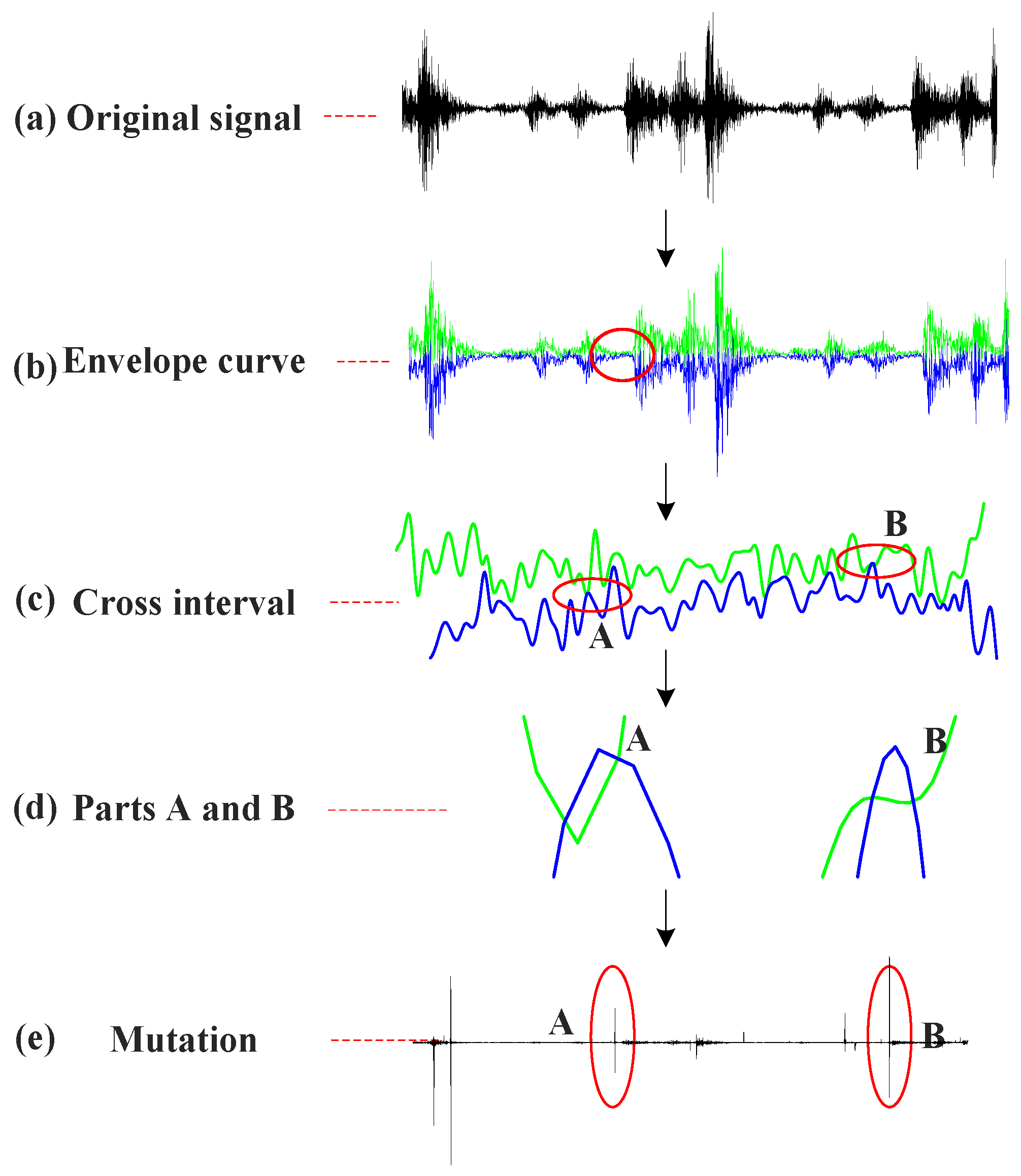
Taking the fault signal of the reciprocating compressor in an oversized bearing clearance state which is shown in Figure 5a as an example, the CSILMD decomposition process is performed to analyze the demodulation mutation phenomenon and its reason. The upper and lower envelopes of the signal shown in Figure 5b are constructed using CSI, and some intervals that occur demodulation mutation phenomenon are enlarged in Figure 5c. It is found that the upper and lower envelopes shown in Figure 5d intersected in these intervals, and we defined these intervals as mutation intervals. In the mutation interval, the upper envelope and lower envelope in CSILMD are nearly equal around the intersection point, resulting in ${\mathrm{a}}_{11}\left(\mathrm{t}\right)$ being equal or extremely close to 0. At this time, the value of this point is substituted into Formula (4) for demodulation, which causes a huge difference between the resulting signal ${\mathrm{h}}_{11}\left(\mathrm{t}\right)$ and the envelope estimation function ${\mathrm{a}}_{11}\left(\mathrm{t}\right)$, and thus the calculation result of the function ${\mathrm{s}}_{11}\left(\mathrm{t}\right)$ does not converge, which results in a demodulation mutation phenomenon. As shown in Figure 5e, two abrupt distortions appear in the mutation intervals of A and B.

2.2.2. Mutation Interval Reconstruction

Based on the above analysis, we think the main reason for the demodulation mutation phenomenon is the intersection of upper and lower envelopes due to local envelope distortion. Therefore, an effective solution needs to be proposed to correct this issue for the stability of the demodulation process.

The envelopes are created using extreme points in the interpolation-based LMD methods such as CSILMD and MPCHILMD. In some local interpolation intervals where the amplitude of the extreme points changes drastically, the information in the extreme point is not enough to ensure the accuracy of the envelope, which leads to the mutation of the envelope. Hence, a direct approach for this issue is to supplement more interpolation points to enrich the envelope construction information in these local interpolation intervals.

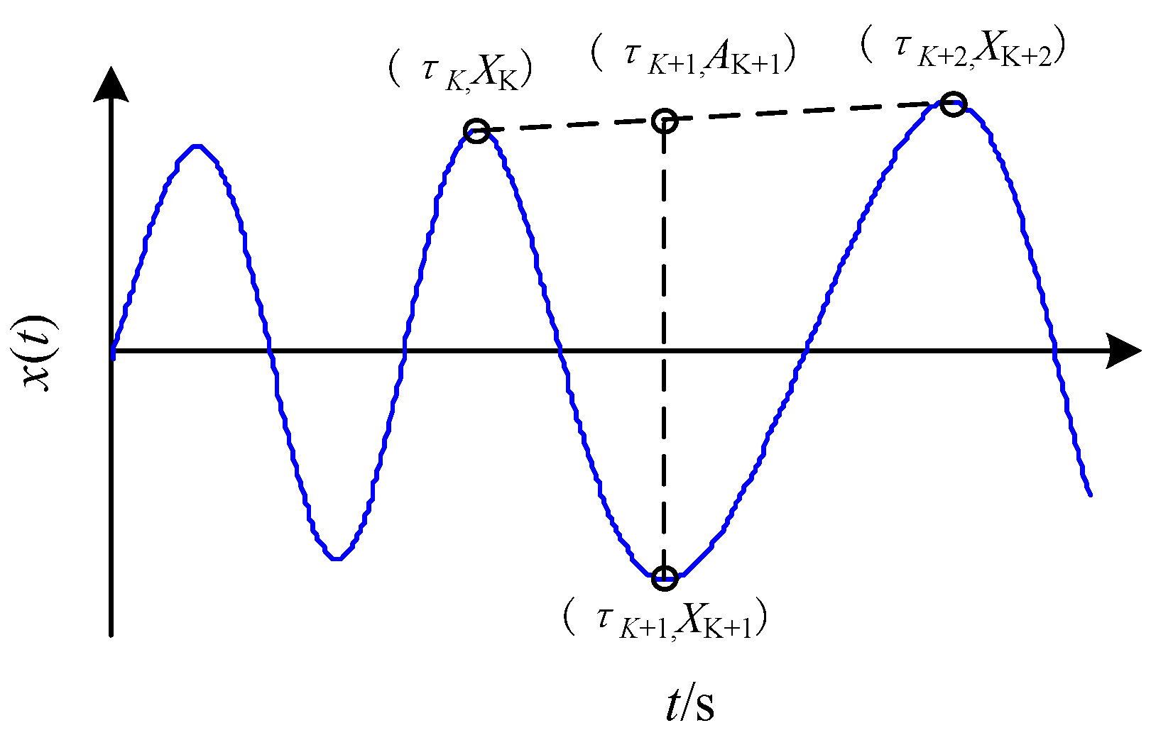
Cheng [33] has proposed the concept of an extreme symmetry point when examining typical single-component signals with clear physical meaning (such as sine, FM, AM, and AM-FM signals) in the local characteristic-scale decomposition (LCD) method. As shown in Figure 6, a straight line is used to connect two adjacent maximum points (${{\mathsf{\tau }}_{\mathrm{k}},\mathrm{X}}_{\mathrm{k}}$) and (${{\mathsf{\tau }}_{\mathrm{k}+2},\mathrm{X}}_{\mathrm{k}+2}$). A point (${{\mathsf{\tau }}_{\mathrm{k}+1},\mathrm{A}}_{\mathrm{k}+1}$) which has the same abscissa position as the minimum point (${{\mathsf{\tau }}_{\mathrm{k}+1},\mathrm{X}}_{\mathrm{k}+1}$) between two adjacent maximum points is given on this line. The point (${{\mathsf{\tau }}_{\mathrm{k}+1},\mathrm{A}}_{\mathrm{k}+1}$) and the minimum point (${{\mathsf{\tau }}_{\mathrm{k}+1},\mathrm{X}}_{\mathrm{k}+1}$) are usually symmetrical about the horizontal axis, and we call this point (${{\mathsf{\tau }}_{\mathrm{k}+1},\mathrm{A}}_{\mathrm{k}+1}$) the extreme symmetry point of the minimum point (${{\mathsf{\tau }}_{\mathrm{k}+1},\mathrm{X}}_{\mathrm{k}+1}$). The specific calculation process of this extreme symmetry point (${{\mathsf{\tau }}_{\mathrm{k}+1},\mathrm{A}}_{\mathrm{k}+1}$) is as follows:

$${\mathrm{A}}_{\mathrm{k}+1}={\mathrm{X}}_{\mathrm{k}}+\frac{{\mathsf{\tau }}_{\mathrm{k}+1}-{\mathsf{\tau }}_{\mathrm{k}}}{{\mathsf{\tau }}_{\mathrm{k}+2}-{\mathsf{\tau }}_{\mathrm{k}}}\left({\mathrm{X}}_{\mathrm{K}+2}-{\mathrm{X}}_{\mathrm{K}}\right)$$

(14)

The PF component is one of the single-component signals with clear physical meaning, and its extreme symmetry points also contain inherent structural information. Therefore, we can employ the extreme symmetry point as interpolation points in these local interpolation intervals to enrich the envelope construction information.

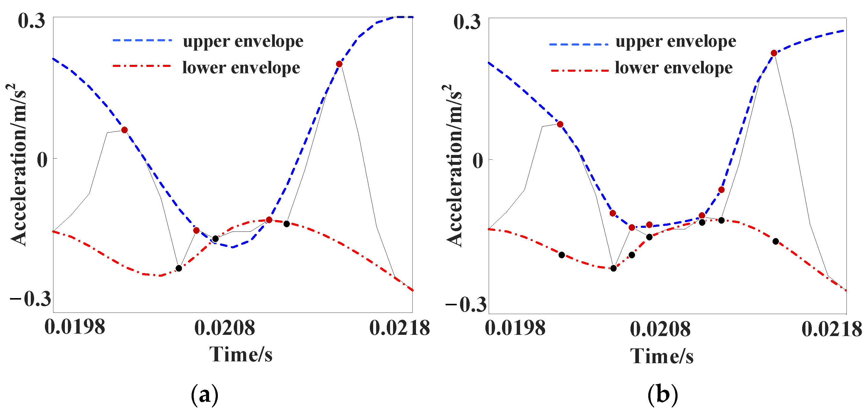
This paper uses extreme symmetry points to supplement the interpolation points of the mutation interval. As shown in Figure 7a, the upper and lower envelopes of a vibration signal from the reciprocating compressor are intersected in the mutation interval, and then the extreme symmetry points are supplemented into the original extreme points. The specific algorithm flow is as follows:

(1)

Calculate the local extreme point sequence ${\mathrm{n}}_{\mathrm{i}}(\mathrm{i}=1,\dots ,\mathrm{w})$ of the signal (${\mathrm{n}}_{\mathrm{i}}$ represents the local maximum point sequence ${\mathrm{n}\mathrm{m}\mathrm{a}\mathrm{x}}_{\mathrm{i}}$ or local minimum point sequence ${\mathrm{n}\mathrm{m}\mathrm{i}\mathrm{n}}_{\mathrm{i}}$), using cubic spline interpolation (or cubic Hermite interpolation) to construct the upper and lower envelope of the signal, and record the first derivative value of the envelope.

(2)

Take the difference between the upper and lower envelope lines to find the local maximum point interval [ ${\mathrm{n}}_{\mathrm{k}},{\mathrm{n}}_{\mathrm{k}+2}]$ and local minimum point interval [ ${\mathrm{n}}_{\mathrm{k}+1},{\mathrm{n}}_{\mathrm{k}+3}$ ] (or [ ${\mathrm{n}}_{\mathrm{k}-1},{\mathrm{n}}_{\mathrm{k}+1}$ ]) of the original signal where the intersection point is located.

(3)

Formula (12) is applied to calculate the extremum augmentation point ${\mathrm{L}}_{\mathrm{i}}$ between the two maxima ${\mathrm{n}}_{\mathrm{k}} \mathrm{and} {\mathrm{n}}_{\mathrm{k}+2}$; calculate the extreme augmentation point ${\mathrm{L}}_{\mathrm{i}}$ between the two minimum points ${\mathrm{n}}_{\mathrm{k}+1} \mathrm{and} {\mathrm{n}}_{\mathrm{k}+3}$ (or ${\mathrm{n}}_{\mathrm{k}-1} \mathrm{and} {\mathrm{n}}_{\mathrm{k}+1}$).

(4)

According to ${\mathrm{n}}_{\mathrm{k}},{\mathrm{L}}_{\mathrm{i}},{\mathrm{n}}_{\mathrm{k}+2}$ and the first derivative value here, cubic Hermite is used to reconstruct the local interval interpolation of the upper envelope; the lower envelope local interval interpolation is reconstructed according to ${\mathrm{n}}_{\mathrm{k}+1},{\mathrm{L}}_{\mathrm{j}},{\mathrm{n}}_{\mathrm{k}+3}$ (or ${\mathrm{n}}_{\mathrm{k}-1},{\mathrm{L}}_{\mathrm{j}},{\mathrm{n}}_{\mathrm{k}+1}$).

(5)

Repeat step (3) and step (4) to reconstruct all the singular intervals in the construction process of the envelope. Finally, connect the reconstructed singular intervals and normal intervals to obtain the processed upper and lower envelope lines.

The upper and lower envelopes of signal in this mutation interval are reconstructed using the supplemented extreme points, and they are shown in Figure 7b. We can know that the envelopes in Figure 7a,b are generally similar in contour, but the envelopes in Figure 7b solve the local envelope crossover problem in Figure 7a, which avoids the case where the envelope estimation function is equal or extremely close to zero, hence solving the demodulation mutation phenomenon. If the reconstructed upper and lower envelopes still have some intersection intervals, we can further supplement the extreme symmetry points to the new mutation intervals until the reconstructed upper and lower envelopes do not intersect.

2.3. Double Interpolation and Mutation Interval Reconstruction Local Mean Decomposition (DIMIRLMD)

2.3.1. DIMIRLMD Scheme

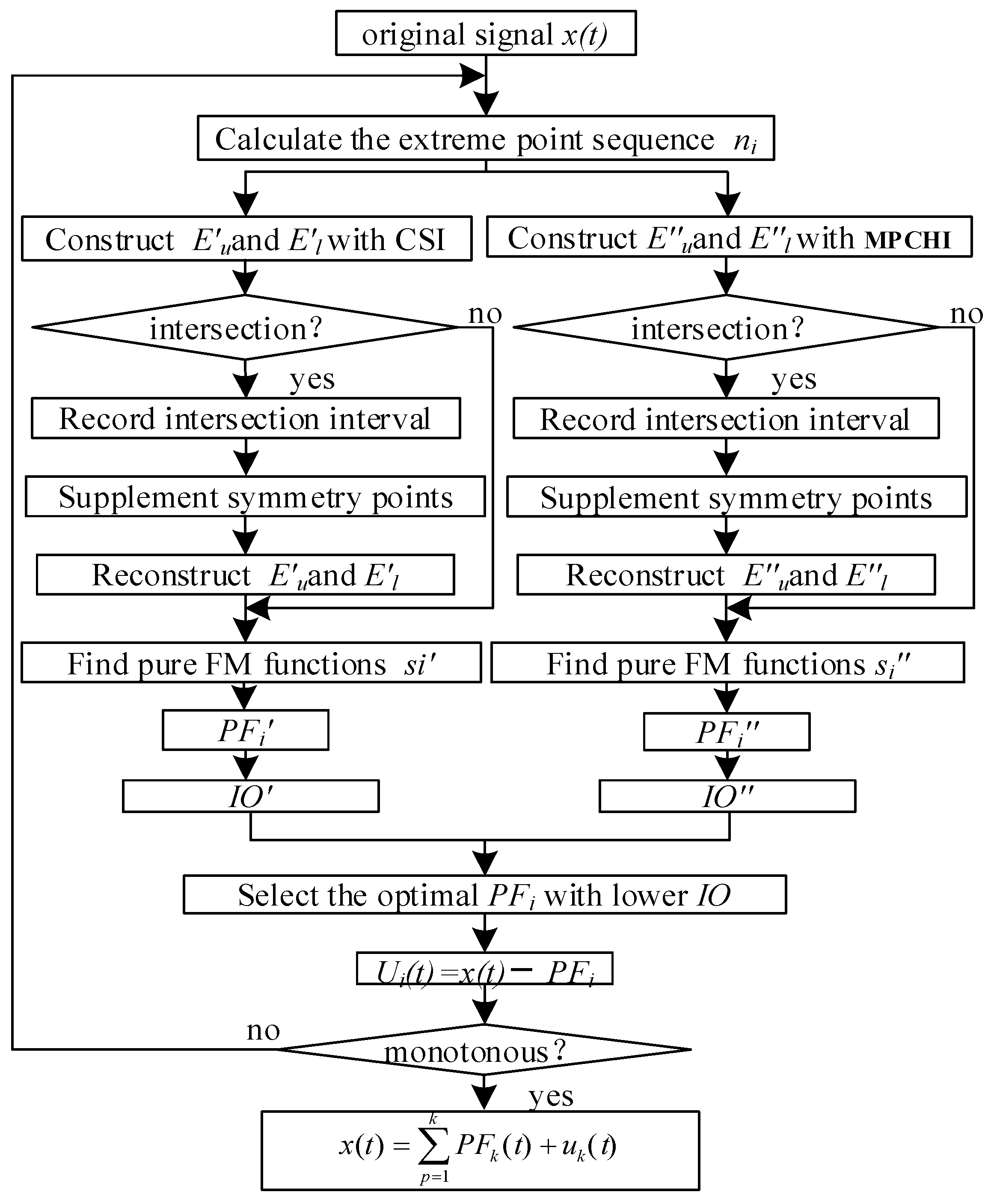
Double interpolation PF optimization and the mutation interval reconstruction envelope are two independent improvements of the LMD algorithm from macro and micro perspectives. The mutation interval reconstruction envelope improves the accuracy of the envelope and the stability of the demodulation process from a micro perspective in each sifting iteration of one PF component. Double interpolation PF optimization is a process for making an optimal selection for each order PF component from a macro perspective for a better hierarchical structure. The implementation process of these two improvements is independent and sequential; that is, these two improvements can be combined within one algorithm to form double interpolation and mutation interval reconstruction local mean decomposition (DIMIRLMD).

In DIMIRLMD, CSI and MPCHI interpolation envelopes are used to demodulate the first-order PF component. No matter which of these two demodulation processes is used, once a demodulation mutation phenomenon occurs in each sifting iteration, the mutation interval will be detected and refreshed with a reconstructed envelope. After the CSI-based PF component and MPCHI-based PF component are obtained, their IO will be calculated. The optimal first-order PF component is selected based on the lower IO. This process is repeated until the residual signal reaches the termination condition, and a series of optimal PF components are obtained.

2.3.2. DIMIRLMD Algorithm

Based on the above analysis, the DIMIRLMD algorithm which integrates the double interpolation PF optimization process and demodulation mutation interval reconstruction process is detailed as follows:

(1)

Calculate the local extreme point sequence of the signal x(t).

(2)

Apply the CSI method to construct the upper envelope ${\mathrm{E}}_{\mathrm{u}}^{\prime }\left(\mathrm{t}\right)$ and lower envelope ${\mathrm{E}}_{\mathrm{u}}^{\prime }\left(\mathrm{t}\right)$ using the extreme point sequence.

(3)

The mutation intervals where the upper and lower envelopes overlap should be determined; add the extreme symmetry points to the original extreme point sequence in the mutation interval to form a new extreme point sequence.

(4)

Reconstruct new envelopes ${\mathrm{E}}_{\mathrm{u}}^{\prime }\left(\mathrm{t}\right)$ and ${\mathrm{E}}_{\mathrm{u}}^{\prime }\left(\mathrm{t}\right)$ with the refreshed extreme point sequence; if the reconstructed envelopes still exhibit mutation intervals, return to step (3) until the exclusion of mutation intervals.

(5)

Calculate the continuous local mean function m₁₁(t) and the envelope function $a_{11}\left(t\right)$ using the reconstructed upper envelope ${\mathrm{E}}_{\mathrm{u}}^{\prime }\left(\mathrm{t}\right)$ and the lower envelope ${\mathrm{E}}_{\mathrm{l}}^{\prime }\left(\mathrm{t}\right)$:

$$m_{11}\left(t\right)=\left(E_u^{\prime }\right(t)+E_l^{\prime }(t\left)\right)/2$$

(15)

$$a_{11}\left(t\right)=\left|E_u^{\prime }\left(t\right)-E_l^{\prime }\left(t\right)\right|/2$$

(16)

(6)

Subtract $m_{11}\left(t\right)$ from the original signal x(t) to obtain ${\mathrm{h}}_{11}\left(\mathrm{t}\right)$, and then the resulting signal ${\mathrm{h}}_{11}\left(\mathrm{t}\right)$ is divided by $a_{11}\left(t\right)$.

$$h_{11}=x\left(t\right)-m_{11}$$

(17)

$$s_{11}\left(t\right)=h_{11}\left(t\right)/a_{11}\left(t\right)$$

(18)

This sifting process continues until s_1n(t) becomes a pure frequency-modulated signal. Multiply a₁(t) by s_1n(t) to obtain the first CSI-based product function ${\mathrm{P}\mathrm{F}}_1^{\prime }\left(\mathrm{t}\right)$ of the original signal:

$${PF}_1^{\prime }\left(t\right)=a_1\left(t\right)s_{1n}\left(t\right)$$

(19)

(7)

Instead of the CSI method, employ the MPCHI method and repeat steps (1) to (6) to obtain the first MPCHI-based product function ${\mathrm{P}\mathrm{F}}_1^{″}\left(\mathrm{t}\right)$ of the original signal.

(8)

Calculate the ${IO}^{\prime }$ of ${\mathrm{P}\mathrm{F}}_1^{\prime \prime }\left(\mathrm{t}\right)$ and ${IO}^{\prime \prime }$ of ${\mathrm{P}\mathrm{F}}_1^{\prime \prime }\left(\mathrm{t}\right)$, and then select the PF component with lower IO as the first optimal PF₁(t) component.

(9)

Subtract PF₁(t) from the original signal x(t) and obtain a new signal u₁(t); the above procedure is repeated k times until u_k becomes a monotonic function, and then we obtain a series of optimal PF components.

The flowchart of the DIMIRLMD algorithm is shown in Figure 8.

3. Results

3.1. Simulated Signal Analysis

To verify the effectiveness of the DIMIRLMD algorithm, a strong nonstationary simulation signal is defined by the superposition of a periodic shock wave, a sinusoidal wave, and noise:

$$\begin{array}{c}y(t)=y_1(t)+y_2(t)+y_3(t)\\ y_1(t)=y_n{e}^{-\xi {\omega }_{n}t}\mathit{sin}{\omega }_n\sqrt{1-{\zeta }^{2}t}\\ \begin{array}{c}{y}_2(t)=y_m\mathit{sin}{\omega }_{m}t\\ y_3(t)=NOISE\end{array}\end{array}$$

(20)

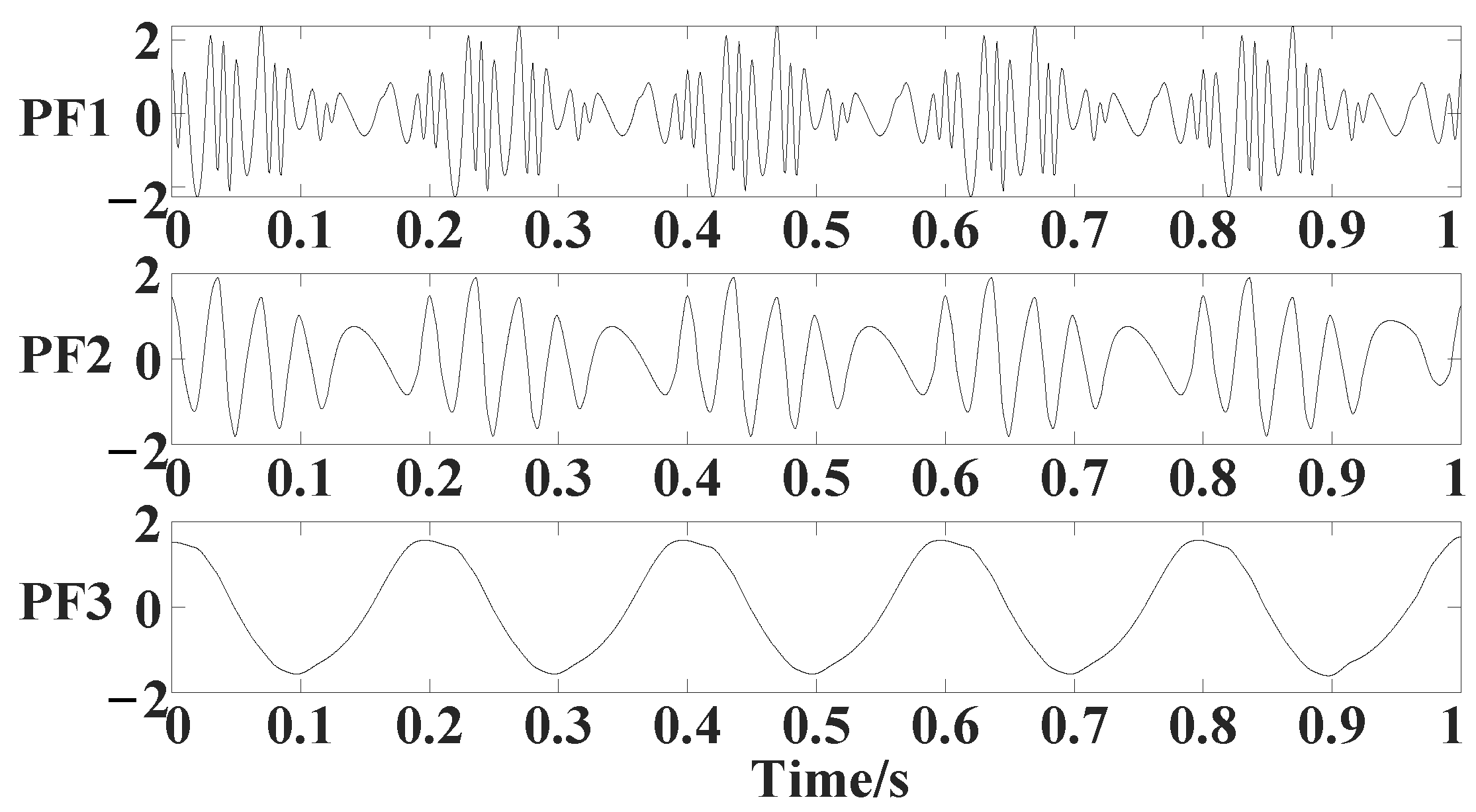
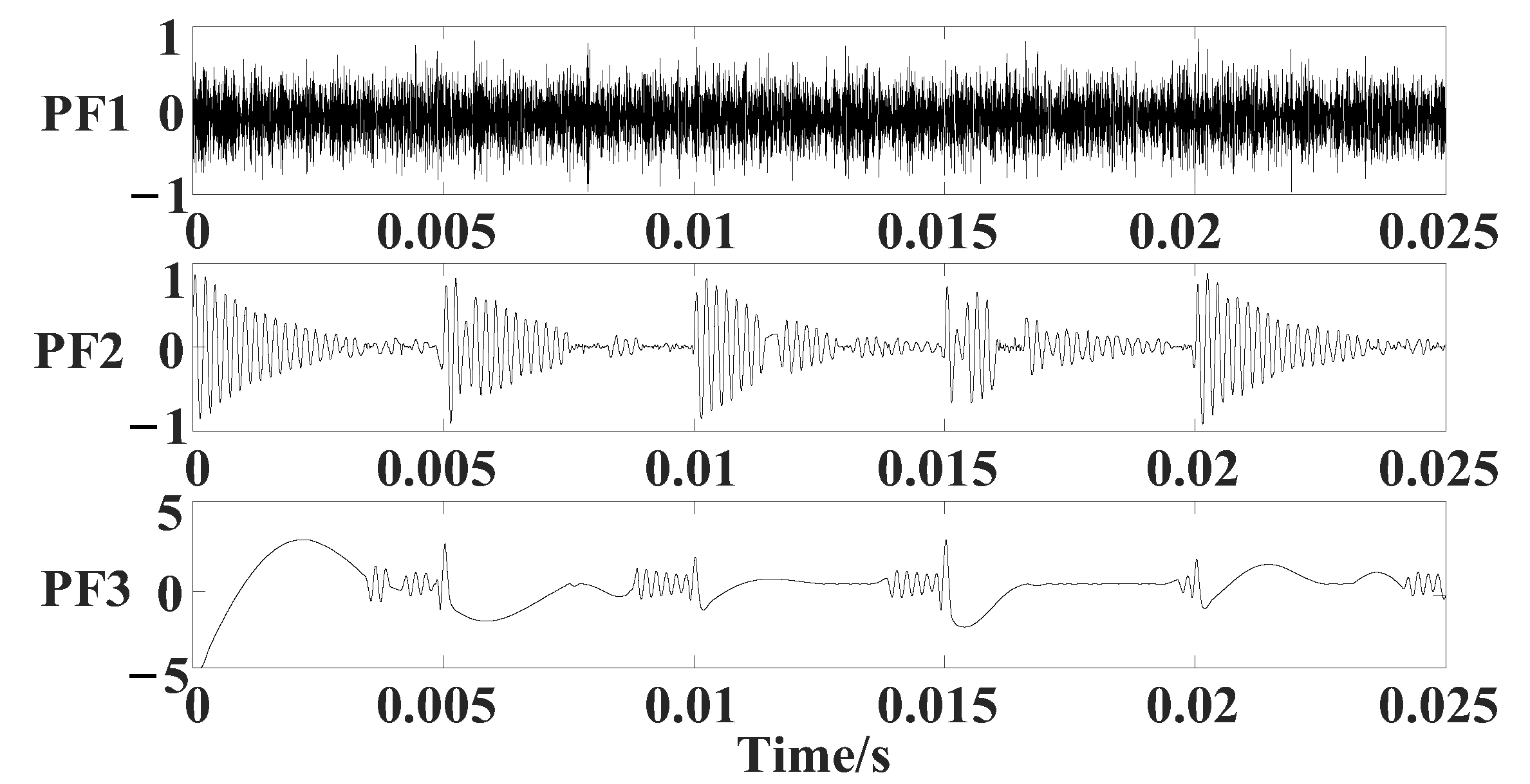
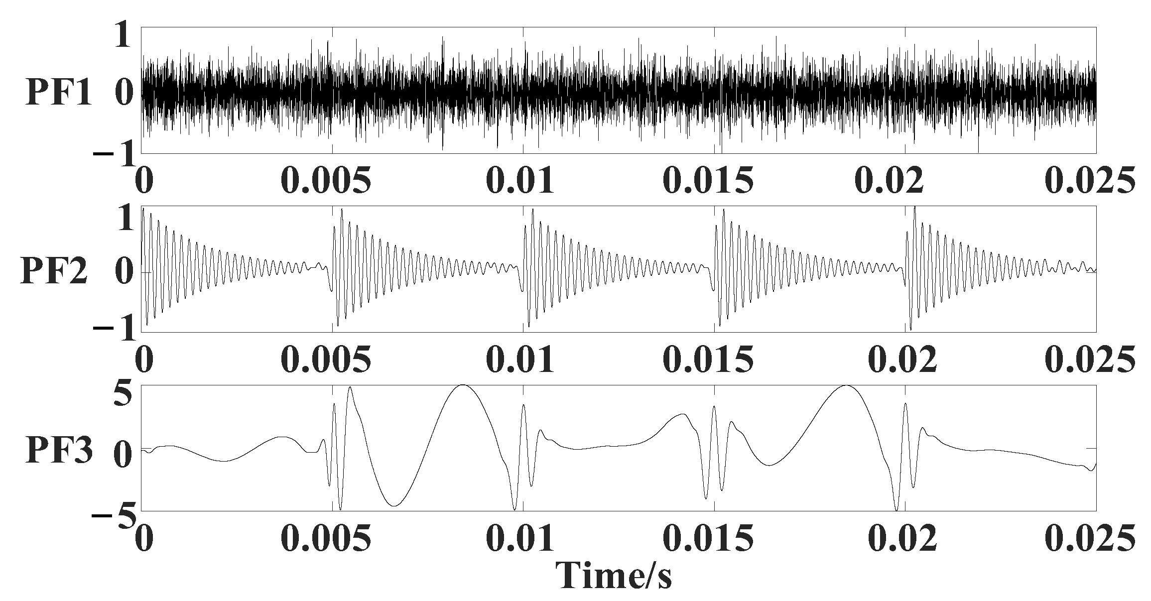
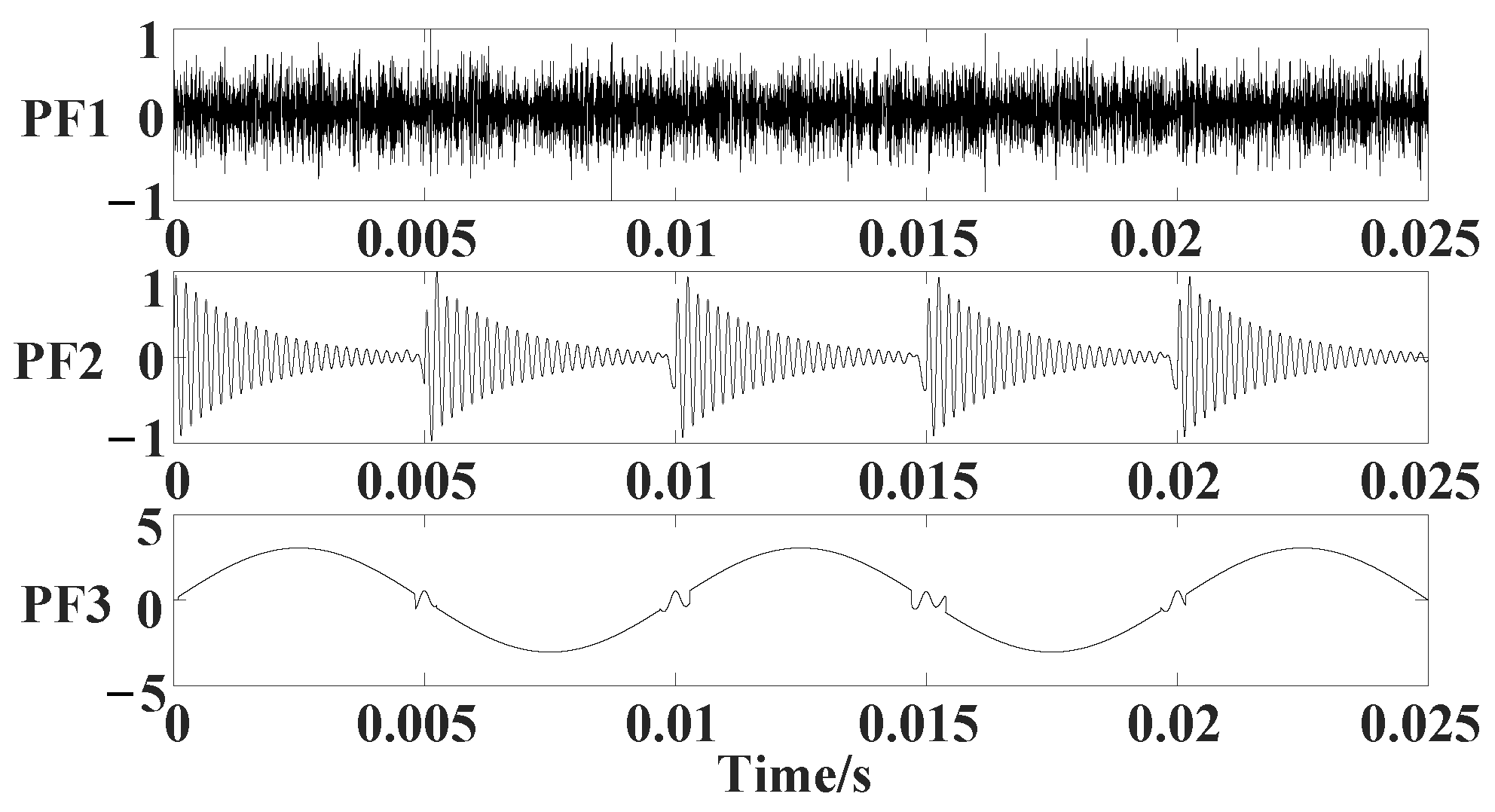
The four methods LMD, CSILMD, MPCHILMD, and DIMIRLMD are each employed to separately break down the signal. The decomposition results of the first three PF components are shown in Figure 9, Figure 10, Figure 11 and Figure 12. In theory, the decomposition results should be decomposed into more than three components from high frequency to low frequency. The noise component should be represented by the first three components, and the impulse component and the sinusoidal component should be contained in the simulation signal.

Through the comparison between decomposition results, significant differences are presented in the four LMD methods. We can see that the second and the third component in Figure 9 for the original LMD have deviated from simulation components, indicating that obvious modal aliasing occurs. The first three components of CSILMD and MPCHILMD are generally similar to the simulation components. Due to the influence of the shock signal, the third sinusoidal PF component of these two methods is mixed with obvious shock disturbance. In the decomposition result of the DIMIRLMD method, although the third component contains a slight shock disturbance, its effect is significantly improved compared with the other three methods.

The most useful assessment metric for different LMD decomposition outputs is the mean square error (MSE) between the PF component and the associated signal. To further compare the analysis results, the MSE of the last two PF components for four LMD methods is shown in

Table 2. Comparison of simulation signal decomposition results with different LMD methods.

Method	PF2		PF3		Time (s)
	MSE	Iterations	MSE	Iterations
LMD	65.482	12	98.994	14	0.871
CSI LMD	25.281	9	14.584	8	0.701
MPCHI LMD	16.203	8	20.420	7	0.677
DIMIR LMD	7.130	5	6.051	5	0.733

. Usually, the more precise the envelope function is, the fewer iterations are needed to complete the decomposition; the iteration number of each PF component is also presented in Table 2.

Corresponding to the conclusions drawn from Figure 9, Figure 10, Figure 11 and Figure 12, Table 2 further proves this fact based on MSE and iterations from a quantitative point of view. Due to serious modal aliasing, the second and third PF components of the original LMD appear to have an excessive MSE and too much iteration compared to the other three methods. CSILMD and MPCHILMD both show a clear improvement in MSE and iterations for two PF components. CSILMD is more excellent in the sinusoidal PF component for its smooth envelope, and MPCHILMD is better in the impulsive PF component for its flexible envelope. The DIMIRLMD presents an outstanding advancement in MSE and iterations for both PF component methods. This is because the optimal double interpolation scheme adaptively matches the best interpolation method for PF components with different characteristics, and the interval reconstruction envelope scheme directly suppresses the demodulation mutation phenomenon. The combination of these two schemes effectively ensures the accuracy and stability of the decomposition.

3.2. Application for Reciprocating Compressor Fault Diagnosis

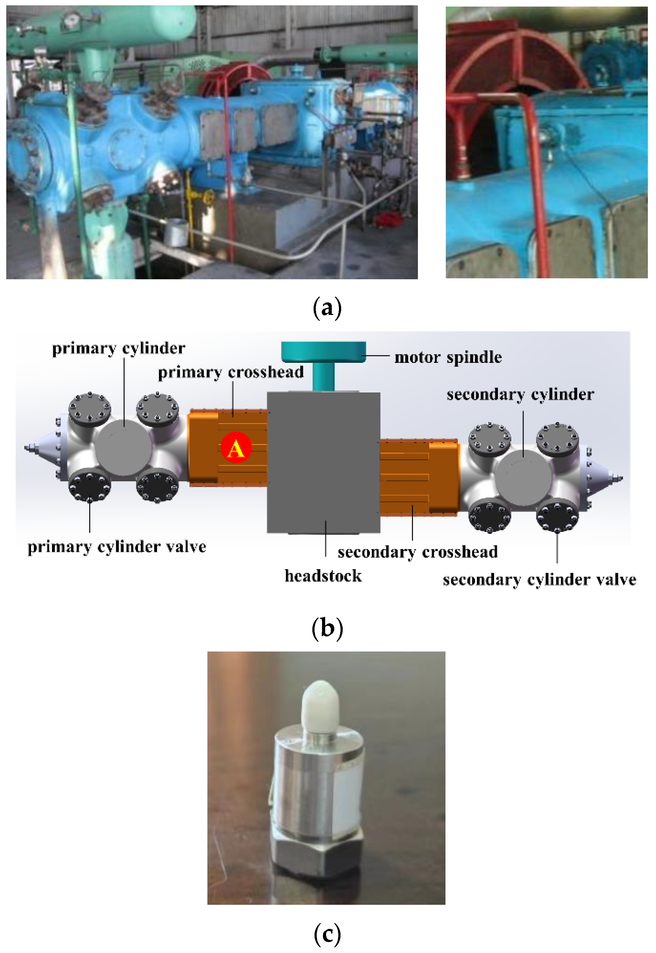
One of the pieces of power equipment that is frequently utilized to compress natural gas for long-distance transportation is the reciprocating compressor. This type of compressor features high efficiency and strong reliability, allowing it to adapt to various operating conditions and environmental situations [34,35]. In this work, the vibration signal of a reciprocating compressor of type 2D12-70 operating with excessive bearing clearance is investigated. The compressed medium is natural gas.

Table 3. Main parameters of 2D12-70 reciprocating compressor.

Parameter Type	Parameter Value
Shaft power (kW)	500
Air displacement (m3/min)	70
Primary exhaust pressure (MPa)	0.2746~0.2942
Secondary exhaust pressure (MPa)	1.2749
Piston stroke (mm)	240
Crank speed (rpm)	496

provides the main parameters of the 2D12-70 reciprocating compressor. The connecting rod in the transmission mechanism connects the crankshaft and crosshead pin with rotate joints, and these joints usually use sliding bearings in the actual structure due to the heavy load. After a long period of friction and wear, the clearance in bearings will increase gradually [36]. Oversized bearing clearances can result in a vibratory operating situation that seriously impairs the performance of the device. Therefore, monitoring and diagnosing excessive bearing clearance effectively and accurately can assist in lowering maintenance costs.

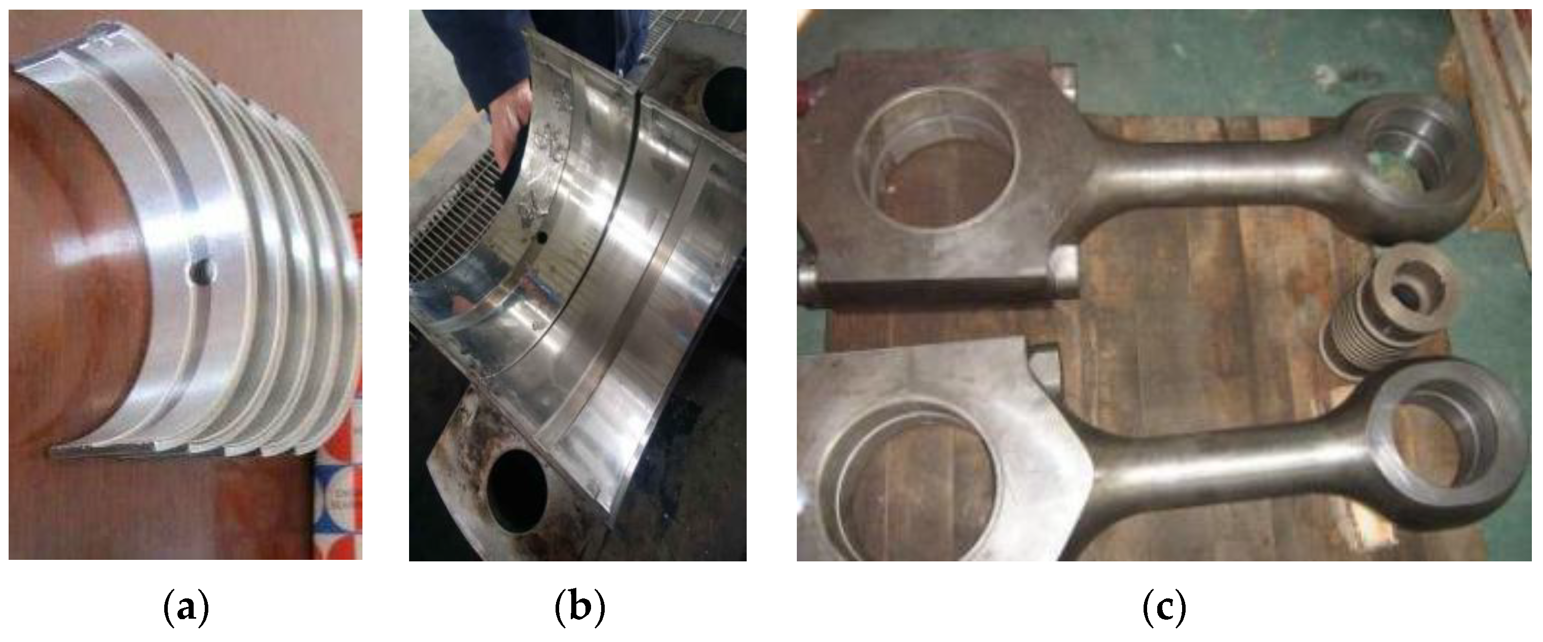
This failure was purposely induced in the bearing between the first-stage crankshaft pin and connecting rod as part of a fault simulation experiment on large bearing clearance states that was carried out in a genuine operating environment. On the cylinder surface during the test, one measuring point was set up to record the vibration signal. Figure 13a,b illustrate the reciprocating compressor and sensor positioning. The test time was 4 s, and the sampling frequency was 50 kHz. Piezoelectric acceleration sensors, specifically model CA-YD-186, were employed. Acceleration sensors are displayed in Figure 13c.

Table 4. Main parameters of CA-YD-186 acceleration sensor.

Parameter Type	Parameter Value
Sensitivity (mV/ms−2)	10.04
Maximum lateral sensitivity ratio (%)	<5
Maximum allowable acceleration (ms−2)	5×102
Electrical property	+
Operating temperature (℃)	−40~120
Working current (mA)	2~10

shows the main parameters of the CA-YD-186 acceleration sensor. Two clearance states, namely a normal clearance state and a medium-worn state, were tested, using a normal bushing in 0.1 mm clearance and a worn bushing in 0.2 mm clearance [37]. The normal and worn bushings and the connecting rod are shown in Figure 14.

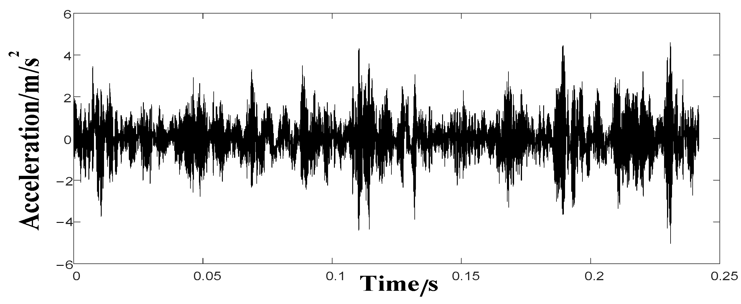
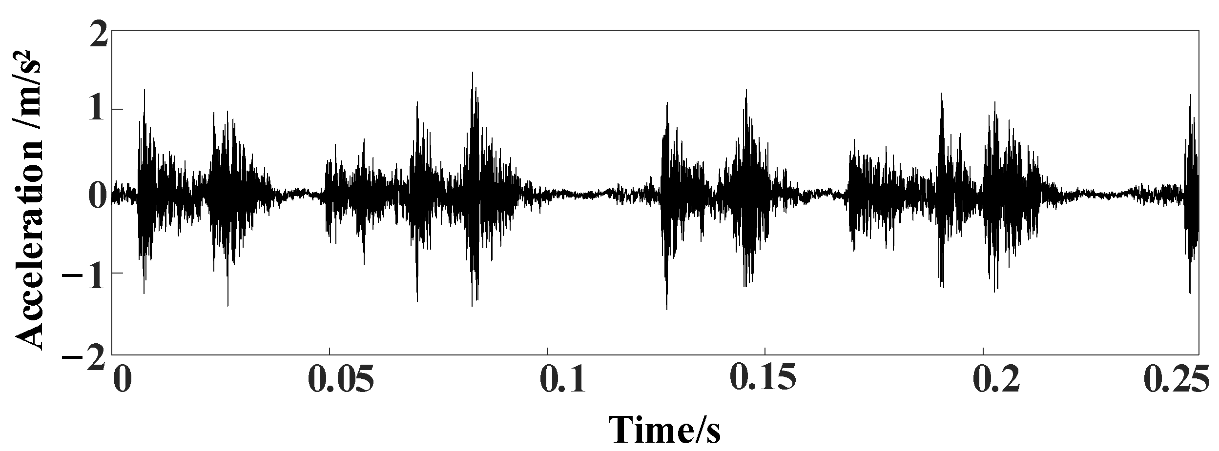
The normal bearing clearance vibration signal is shown in Figure 15. The vibration signal in the oversized bearing clearance state is shown in Figure 16. When an oversized clearance arises in the bearing, strong contact forces are excited due to the direct impact between the journal and bushing. The journal and bushing usually impact twice for their relative movement direction change two times in one rotation period, and these strong contact forces lead to a peak on double rotation frequency in the envelope frequency spectrum as shown in Figure 17. The vibration signals of the reciprocating compressor, however, may exhibit many interference frequencies due to the nonlinear factors such as clearance and stiffness present in the complex vibration transmission path. This submerges the double rotation frequency caused by bearing clearance and prevents the accurate identification of fault information. As a result, reliable identification of the large bearing clearance status from the noisy vibration signal requires the use of a suitable feature extraction approach, such as LMD.

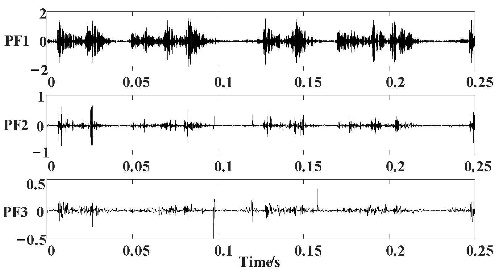
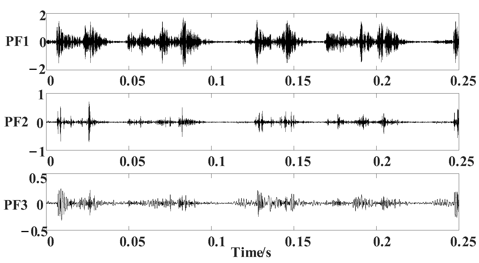
Usually, the main fault information is contained in the first several PF components, so the first three PF components are given in Figure 18, Figure 19, Figure 20 and Figure 21 for four LMD methods. We can see that the periodical shocks caused by bearing clearance dominate the first PF component and that the frequency and amplitude steadily decrease in the succeeding PF components. The mutation of the envelope estimation function causes a significant distortion in the second and third PF components of CSILMD. The decomposition results of LMD and MPCHILMD have some local distortion in their second and third PF components, and those of the DIMIRLMD are relatively stable.

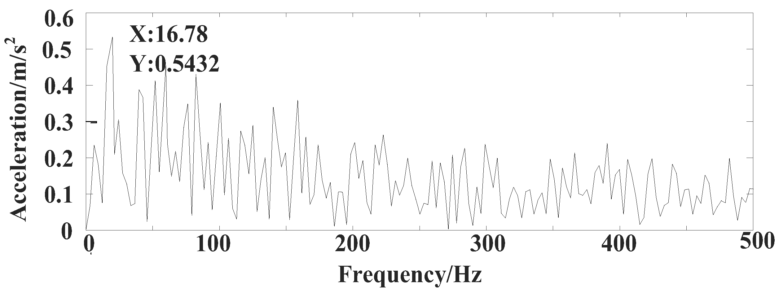
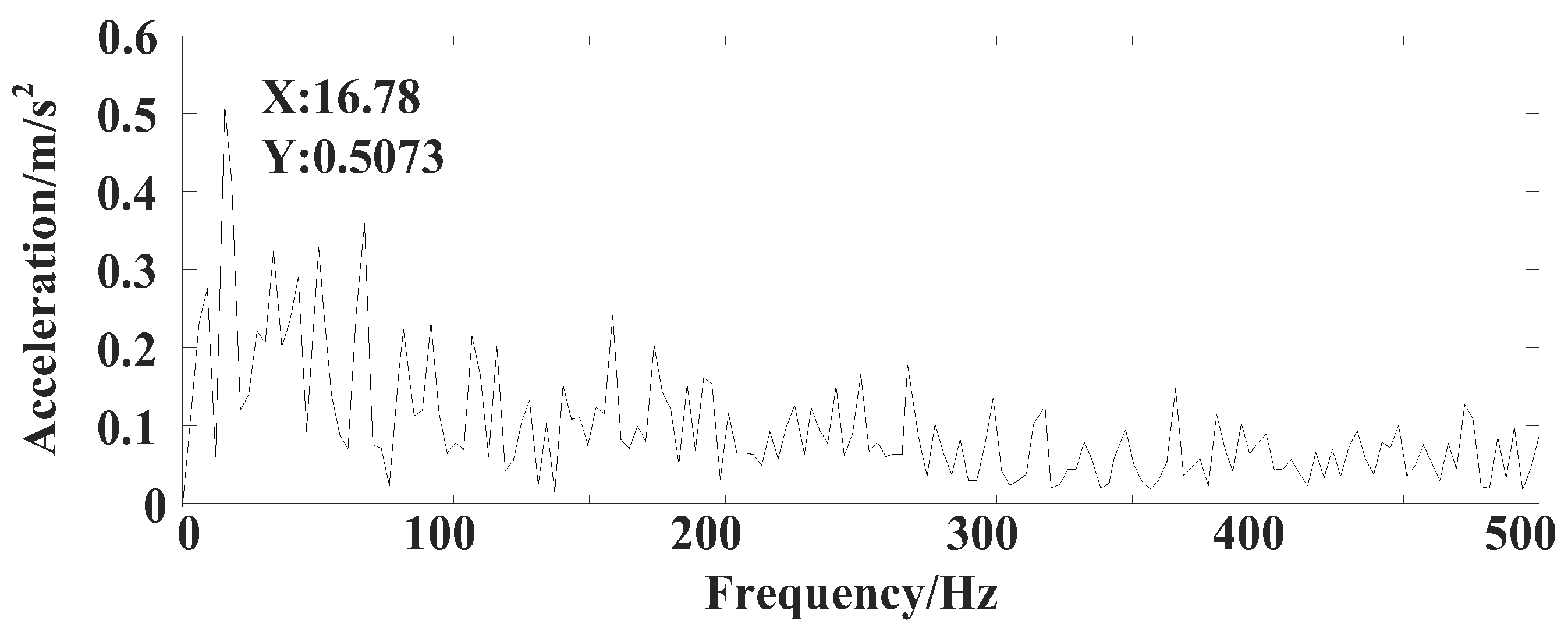
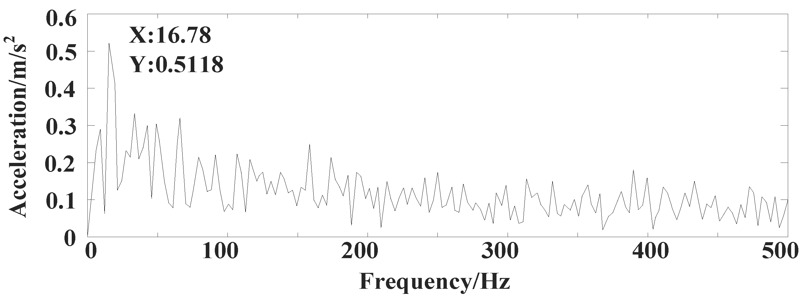
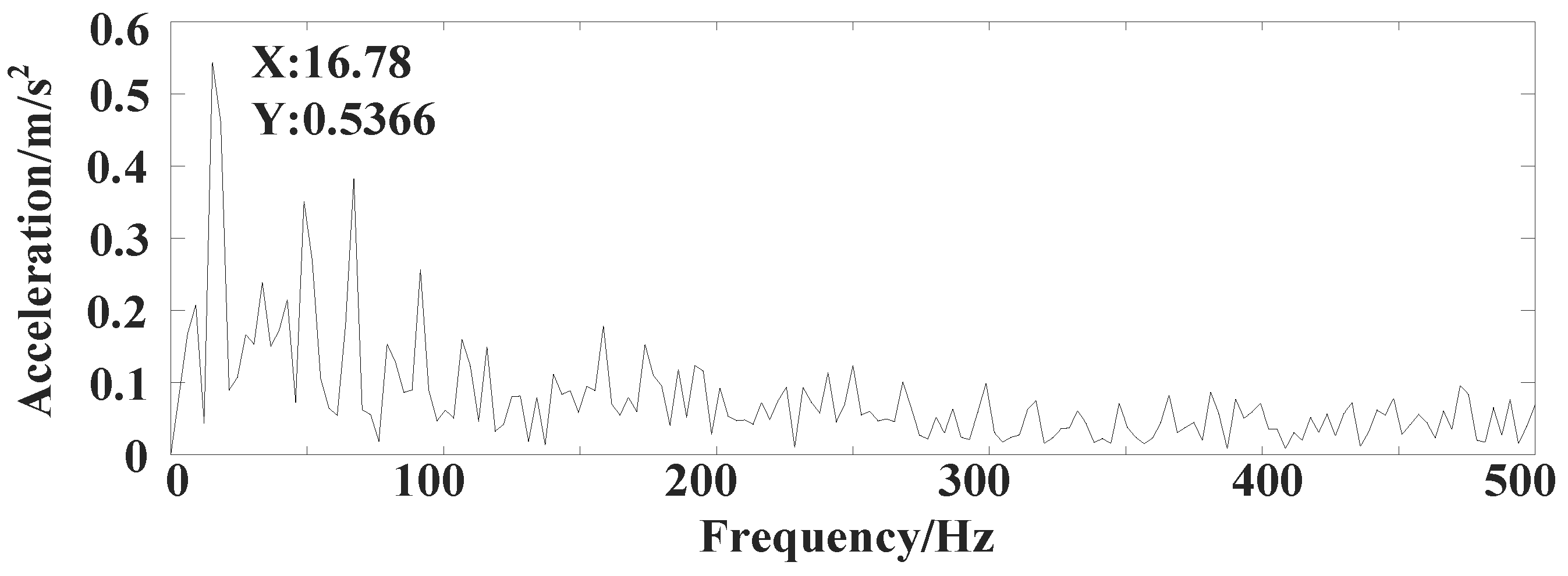
In Figure 22, Figure 23, Figure 24 and Figure 25 four LMD approaches’ envelope frequency spectra for the first PF component are provided. The interference frequencies are further suppressed compared to the original envelope frequency spectrum in Figure 17 because some interference frequencies are eliminated during the LMD decomposition process. They all exhibit a distinct peak in the double rotation frequency and several gradually attenuated multi-rotation frequencies. The peak value refers to the difference between the highest or lowest value of the signal and the average value in a period. According to Formula (21), the peak index which is defined as the ratio between the peak value in double rotation frequency and root mean square (RMS) is employed to compare performance differences of the envelope frequency spectrum.

$$Peak Index=\frac{P}{RMS}$$

(21)

The five envelope frequency spectra are derived from the original signal and the first PF component of four LMDs, and the peak index, peak value in double rotation frequency, and RMS value of each are displayed in

Table 5. Comparison of index values of envelope frequency spectrum for various LMD methods.

Index Value	Method
	Original	LMD	CSI LMD	MPCHI LMD	DIMIRLMD
Peak Value	0.5432	0.5121	0.5073	0.5118	0.5336
RMS Value	0.1521	0.0824	0.0728	0.0695	0.0652
Peak Index	3.5713	6.2148	6.9684	7.3640	8.1840

in that order. The peak and the RMS value of the original envelope frequency spectrum are the highest in the five spectra, while the peak index is the lowest, which indicates the fault information is submerged in the background noise seriously. The peak and the RMS value of the envelope frequency spectrum for four PF components are both lower than those of the original one, but the peak index is significantly higher, and this verifies that LMD is an effective approach for extracting fault frequency. In these four PF envelope frequency spectra, the DIMIRLMD has the greatest peak index and peak value, demonstrating that it successfully suppresses the interference frequency in addition to more fully retaining fault frequency.

Table 6. Comparison of decomposition results of different LMD methods.

Method	Iteration	IO	$\mathit{I}\mathit{E}\mathit{C}$
	PF1  PF2  PF3	PF1  PF2  PF3
LMD	7.121 6.487 5.846 ±1.311 ±1.552 ±1.648	0.315 0.346 0.415 ±0.052 ±0.081 ±0.074	0.811 ±0.098
CSI LMD	5.943 10.434 9.567 ±1.225 ±1.965 ±1.841	0.253 0.537 0.695 ±0.053 ±0.086 ±0.093	0.874 ±0.086
MPCHI LMD	5.454 4.454 5.524 ±0.891 ±1.078 ±1.447	0.185 0.243 0.286 ±0.049 ±0.054 ±0.065	0.887 ±0.072
DIMIR LMD	4.665 3.823 3.735 ±0.628 ±0.752 ±0.848	0.177 0.232 0.273 ±0.046 ±0.051 ±0.058	0.905 ±0.048

provides the mean value and 3 times the standard deviation of iterations for the first three PF components to further illustrate the effectiveness of DIMIRLMD with quantitative indicators. Twenty sample signals in an oversized bearing clearance fault state were decomposed using four different LMD methods. As previously mentioned, the more precise the envelope function is, the fewer iterations are needed to complete the decomposition. We can see that DIMIRLMD has the lowest mean value and the smallest standard deviation of iterations for each PF component, which indicates a higher accuracy of the envelope function and a better immunity to noise interference.

Similar to the average index of orthogonality (IO), the index of energy conservation (IEC) is also a widely used index to evaluate the performance of various self-adaptive decomposition methods [38]. The energy of the original signal and its PF components should be conservative; hence, the IEC is equal to 1 in theory. The mean value and 3 times the standard deviation of IO and IEC for the four LMD methods are also presented in Table 6. We can know that DIMIRLMD has the lowest mean value and the smallest standard deviation of IO for each order PF component, which illustrates DIMIRLMD has the best PF component hierarchical structure. Furthermore, the mean value of IEC is closer to 1 than those of the other three LMD methods. The aforementioned findings also suggest that DIMIRLMD is effective in extracting fault features from signals with nonstationary characteristics and significant noise interference, particularly vibration signals from reciprocating compressors operating with excessive bearing clearance.

4. Conclusions

Double interpolation PF optimization and the mutation interval reconstruction envelope are two independent improvements of LMD, and this paper combines the two improvements in one algorithm to form double interpolation and mutation interval reconstruction local mean decomposition (DIMIRLMD).

(1)

The main reason for the demodulation mutation phenomenon is found to be the intersection of upper and lower envelopes, and the extreme symmetry points are employed to reconstruct the envelopes. The mutation interval reconstruction algorithm effectively suppressed the demodulation mutation phenomenon.

(2)

Two typical interpolation envelope methods, CSI and MPCHI, are used to obtain PF components, and then the optimal PF component is selected based on the index of orthogonality (IO). Double interpolation PF optimization achieves a better hierarchical property for each order PF component. The orthogonality of decomposition results is improved, and the accuracy of the PF component is guaranteed.

(3)

A numerical simulation experiment indicated that DIMIRLMD outperforms the other three LMD methods in MSE and sifting iterations of PF components. The fault characteristics of the strong nonstationary vibration signal of the reciprocating compressor are more accurately quantified.

(4)

DIMIRLMD was applicated in feature extraction from the vibration signals of the reciprocating compressor in an oversized bearing clearance fault state; results show it is superior in the sifting iterations, IO, and IEC compared to the other three LMD methods. Furthermore, the significant peak index of the PF component envelope frequency spectrum verified the superiority of DIMIRLMD in increased reciprocating pressure compressor fault identification accuracy.

References

1. Chen, X.; Wang, S.; Qiao, B.; Chen, Q. Basic research on machinery fault diagnostics: Past, present, and future trends. Front. Mech. Eng. 2018, 13, 264–291. [Google Scholar] [CrossRef] [Green Version]
2. Zhao, H.; Wang, J.; Lee, J.; Li, Y. A compound interpolation envelope local mean decomposition and its application for fault diagnosis of reciprocating compressors. Mech. Syst. Signal Process. 2018, 110, 273–295. [Google Scholar]
3. Feng, Z.; Liang, M.; Chu, F. Recent advances in time–frequency analysis methods for machinery fault diagnosis: A review with application examples. Mech. Syst. Signal Process. 2013, 38, 165–205. [Google Scholar] [CrossRef]
4. Rachna, V.; Saurabh, D.U.D.; Tripathi, S.M. Machine learning applications in power system fault diagnosis: Research advancements and perspectives. Eng. Appl. Artif. Intell. 2021, 106, 104504. [Google Scholar]
5. Zhao, N.; Zhang, J.; Mao, Z.; Jiang, Z. Variational time–frequency adaptive decomposition of machine multi-impact vibration signals. Mech. Syst. Signal Process. 2023, 189, 110084. [Google Scholar] [CrossRef]
6. Sharma, V.; Parey, A. Performance evaluation of decomposition methods to diagnose leakage in a reciprocating compressor under limited speed variation. Mech. Syst. Signal Process. 2019, 125, 275–287. [Google Scholar] [CrossRef]
7. Zhang, Y.; Yang, G.; Zhang, D.; Wang, T. Investigation on recognition method of acoustic emission signal of the compressor valve based on the deep learning method. Energy Rep. 2021, 7, 62–71. [Google Scholar] [CrossRef]
8. Zhang, Y.; Ji, J.; Ma, B. Fault diagnosis of reciprocating compressor using a novel ensemble empirical mode decomposition-convolutional deep belief network. Measurement 2020, 156, 107619. [Google Scholar] [CrossRef]
9. Cabrera, D.; Guamán, A.; Zhang, S.; Cerrada, M.; Sánchez, R.-V.; Cevallos, J.; Long, J.; Li, C. Bayesian approach and time series dimensionality reduction to LSTM-based model-building for fault diagnosis of a reciprocating compressor. Neurocomputing 2020, 380, 51–66. [Google Scholar] [CrossRef]
10. Lv, Q.; Cai, L.; Yu, X.; Ma, H.; Li, Y.; Shu, Y. An Automatic Fault Diagnosis Method for the Reciprocating Compressor Based on HMT and ANN. Appl. Sci. 2022, 12, 5182. [Google Scholar] [CrossRef]
11. Li, Y.; Pan, Y.; Ba, P.; Wu, S.; Chen, J. Fault Feature Extraction Method of Reciprocating Compressor Valve Based on SPA-MF. IEEE Access 2022, 10, 127182–127191. [Google Scholar] [CrossRef]
12. Norden, E. The Empirical Mode Decomposition and the Hilbert Spectrum for Nonlinear and Non-Stationary Time Series Analysis. Proc. R. Soc. A Mathmatical Phys. Eng. Sci. 1998, 454, 903–995. [Google Scholar]
13. Jonathan, S. The Local Mean Decomposition and Its Application to EEG Perception Data. J. R. Soc. Interface 2022, 2, 443–454. [Google Scholar]
14. Dragomiretskiy, K.; Zosso, D. Variational Mode Decomposition. IEEE Trans. Signal Process. 2014, 62, 531–544. [Google Scholar] [CrossRef]
15. Rohit, M.; Bhagat, S. Stability analysis in milling process using spline based local mean decomposition (SBLMD) technique and statistical indicators. Measurement 2021, 174, 108999. [Google Scholar]
16. Ezzat, D.; Hassanien, A.; Darwish, A.; Yahia, M.; Ahmed, A.; Abdelghafar, S. Multi-Objective Hybrid Artificial Intelligence Approach for Fault Diagnosis of Aerospace Systems. IEEE Access 2021, 9, 41717–41730. [Google Scholar] [CrossRef]
17. Wang, J.; Li, J.; Wang, H.; Jiaqiang, E. Research on gearbox composite fault diagnosis based on improved local mean decomposition. Int. J. Dyn. Control. 2021, 9, 1411–1422. [Google Scholar] [CrossRef]
18. Liu, Z.; Zuo, M.J.; Jin, Y.; Pan, D.; Qin, Y. Improved local mean decomposition for modulation information mining and its application to machinery fault diagnosis. J. Sound Vib. 2017, 397, 266–281. [Google Scholar] [CrossRef]
19. Guo, W.; Huang, L.; Chen, C.; Zou, H.; Liu, Z. Elimination of End Effects in Local Mean Decomposition Using Spectral Coherence and Applications for Rotating Machinery. Digit. Signal Process. 2016, 55, 52–63. [Google Scholar] [CrossRef]
20. Li, Y.; Liang, X.; Yang, Y.; Xu, M.; Huang, W. Early Fault Diagnosis of Rotating Machinery by Combining Differential Rational Spline-Based LMD and K–L Divergence. IEEE Trans. Instrum. Meas. 2017, 66, 3077–3099. [Google Scholar] [CrossRef]
21. Yang, Y.; Cheng, J.; Zhang, K. An ensemble local means decomposition method and its application to local rub-impact fault diagnosis of the rotor systems. Measurement 2012, 45, 561–570. [Google Scholar] [CrossRef]
22. Li, Y.; Si, S.; Liu, Z.; Liang, X. Review of local mean decomposition and its application in fault diagnosis of rotating machinery. J. Syst. Eng. Electron. 2019, 30, 799–814. [Google Scholar]
23. Yang, S.; Hu, J.; Mao, Z.; Wu, S. Empirical Mode Decomposition Based on Higher Order Spline interpolation. Zhejiang Univ. 2004, 3, 12–15. [Google Scholar]
24. Liao, M.; Liu, C.; Wang, C.; Yang, J. Research on a Rolling Bearing Fault Detection Method With Wavelet Convolution Deep Transfer Learning. IEEE Access 2021, 9, 45175–45188. [Google Scholar] [CrossRef]
25. Zhang, Y.; Li, S.; Zhang, A.; Li, C.; Qiu, L. A Novel Bearing Fault Diagnosis Method Based on Few-Shot Transfer Learning across Different Datasets. Entropy 2022, 24, 1295. [Google Scholar] [CrossRef] [PubMed]
26. Cheng, G.; Li, H.; Hu, X.; Chen, X.; Liu, H. Fault diagnosis of gearbox based on local mean decomposition and discrete hidden Markov models. Proc. Inst. Mech. Eng. Part C J. Mech. Eng. Sci. 2016, 231, 2706–2717. [Google Scholar] [CrossRef]
27. Cheng, J.; Zhang, K.; Yang, Y. An order tracking technique for the gear fault diagnosis using local mean decomposition method. Mech. Mach. Theory 2012, 55, 67–76. [Google Scholar] [CrossRef]
28. Liu, Z.-H.; Lu, B.-L.; Wei, H.-L.; Chen, L.; Li, X.-H.; Wang, C.-T. A Stacked Auto-Encoder Based Partial Adversarial Domain Adaptation Model for Intelligent Fault Diagnosis of Rotating Machines. IEEE Trans. Ind. Informatics 2021, 17, 6798–6809. [Google Scholar] [CrossRef]
29. Ye, X.; Wang, P.; Yang, Z. Time Sequential Phase Partition and Modeling Method for Fault Detection of Batch Processes. IEEE Access 2018, 6, 1249–1260. [Google Scholar] [CrossRef]
30. Qin, Y.; Zou, J.; Cao, F. Adaptively Detecting the Transient Feature of Faulty Wind Turbine Planetary Gearboxes by the Improved Kurtosis and Iterative Thresholding Algorithm. IEEE Access 2018, 6, 14602–14612. [Google Scholar] [CrossRef]
31. Pu, X.; Li, C. Online Semi-Supervised Broad Learning System for Industrial Fault Diagnosis. IEEE Trans. Ind. Inform. 2021, 17, 6644–6654. [Google Scholar] [CrossRef]
32. Mezni, Z.; Delpha, C.; Diallo, D.; Braham, A. Performance of Bearing Ball Defect Classification Based on the Fusion of Selected Statistical Features. Entropy 2022, 24, 1251. [Google Scholar] [CrossRef] [PubMed]
33. Li, L.; Guo, A.; Chen, H. Feature Extraction Based on EWT With Scale Space Threshold and Improved MCKD for Fault Diagnosis. IEEE Access 2021, 9, 45407–45417. [Google Scholar] [CrossRef]
34. Zhang, Y.; Zhang, L. Intelligent fault detection of reciprocating compressor using a novel discrete state space. Mech. Syst. Signal Process. 2022, 169, 108583. [Google Scholar] [CrossRef]
35. Sim, H.Y.; Ramli, R.; Saifizul, A.; Soong, M.F. Detection and estimation of valve leakage losses in reciprocating compressor using acoustic emission technique. Measurement 2020, 152, 107315. [Google Scholar] [CrossRef]
36. Song, M.; Wang, J.; Zhao, H.; Li, Y. Bearing failure of reciprocating compressor sub-health recognition based on CAGOA-VMD and GRCMDE. Adv. Mech. Eng. 2022, 14, 168781322210829. [Google Scholar] [CrossRef]
37. Song, Y.; Wang, W. A Fault Feature Extraction Method for Rolling Bearings Based on Refined Composite Multi-Scale Amplitude-Aware Permutation Entropy. IEEE Access 2021, 9, 71979–71993. [Google Scholar] [CrossRef]
38. Ma, J.; Zhuo, S.; Li, C.; Zhan, L.; Zhang, G. An Enhanced Intrinsic Time-Scale Decomposition Method Based on Adaptive Lévy Noise and Its Application in Bearing Fault Diagnosis. Symmetry 2021, 13, 617. [Google Scholar] [CrossRef]
Figure 1. Flowchart of interpolation-based LMD.
Applsci 13 07543 g001
Figure 2. Simulation signal X and its components.
Applsci 13 07543 g002
Figure 3. CSILMD decomposition results of simulation signal.
Applsci 13 07543 g003
Figure 4. MPCHILMD decomposition results of simulation signal.
Applsci 13 07543 g004
Figure 5. Demodulation mutation phenomenon.(a) Original signal (b) Envelope curve (c) Cross interval (d) Parts A and B (e) Mutation.
Applsci 13 07543 g005
Figure 6. AM-FM signal.
Applsci 13 07543 g006
Figure 7. Comparison of mutation interval reconstruction. (a) Intersected envelopes in mutation interval. (b) Envelopes reconstructed in mutation interval.
Applsci 13 07543 g007
Figure 8. Flowchart of DIMIRLMD.
Applsci 13 07543 g008
Figure 9. LMD decomposition result of simulation signal.
Applsci 13 07543 g009
Figure 10. CSILMD decomposition result of simulation signal.
Applsci 13 07543 g010
Figure 11. MPCHILMD decomposition result of simulation signal.
Applsci 13 07543 g011
Figure 12. DIMIRLMD decomposition result of simulation signal.
Applsci 13 07543 g012
Figure 13. Reciprocating compressor fault test platform. (a) Reciprocating compressor and sensor location. (b) Sensor location of 3D model. (c) CA-YD-186 acceleration sensor.
Applsci 13 07543 g013
Figure 14. Connecting rod and bearing bushing for oversized clearance fault test. (a) Normal clearance bushing. (b) Medium-worn bushing. (c) Connecting rod.
Applsci 13 07543 g014
Figure 15. Vibration signal of reciprocating compressor in normal bearing clearance.
Applsci 13 07543 g015
Figure 16. Vibration signal of reciprocating compressor in oversized bearing clearance.
Applsci 13 07543 g016
Figure 17. Envelope frequency spectrum of fault signal.
Applsci 13 07543 g017
Figure 18. LMD decomposition result of fault signal.
Applsci 13 07543 g018
Figure 19. CSILMD decomposition result of fault signal.
Applsci 13 07543 g019
Figure 20. MPCHILMD decomposition result of fault signal.
Applsci 13 07543 g020
Figure 21. DIMIRLMD decomposition result of fault signal.
Applsci 13 07543 g021
Figure 22. Envelope frequency spectrum of first PF1 in LMD.
Applsci 13 07543 g022
Figure 23. Envelope frequency spectrum of first PF1 in CSILMD.
Applsci 13 07543 g023
Figure 24. Envelope frequency spectrum of first PF1 in MPCHILMD.
Applsci 13 07543 g024
Figure 25. Envelope frequency spectrum of first PF1 in DIMIRLMD.
Applsci 13 07543 g025