Transformer Fault Diagnosis Method Based on Incomplete Data and TPE-XGBoost

Abstract

Dissolved gas analysis is an important method for diagnosing the operating condition of power transformers. Traditional methods such as IEC Ratios and Duval Triangles and Pentagon methods are not applicable in the case of abnormal or missing values of DGA data. A novel transformer fault diagnosis method based on an extreme gradient boosting algorithm is proposed in this paper. First, the traditional statistical method is replaced by the random forest regression algorithm for filling in missing values of dissolved gas data. Normalization and feature derivation of the outlier data is adopted based on the gas content. Then, hyperparameter optimization of the transformer fault diagnosis model based on an extreme gradient boosting algorithm is carried out using the tree-structured probability density estimator algorithm. Finally, the influence of missing data and optimization algorithms on transformer fault diagnosis models is analyzed. The effects of different algorithms based on incomplete datasets are also discussed. The results show that the performance of the random forest regression algorithm on missing data filling is better than classification and regression trees and traditional statistical methods. The average accuracy of the fault diagnosis method proposed in the paper is 89.5%, even when the missing data rate reaches 20%. The accuracy and robustness of the TPE-XGBoost model are superior to other machine learning algorithms described in this paper, such as k-nearest neighbor, deep neural networks, random forest, etc.

1. Introduction

Transformers are one of the key equipment in the power system, and their operating status will directly affect the safety and stability of the system. The number of transformers in a power system is related to the size of the system, and the service life of different transformers varies widely. With the extension of service life, problems such as insulation aging or internal defects will inevitably appear. Therefore, real-time monitoring of transformer operation status and fault warning is extremely important to enhance the safety and stability of the power system [1].

Dissolved gas analysis (DGA) is one of the most important methods for understanding the health of transformers. Without affecting the normal operation of the transformer, internal defects of the transformer can be identified according to changes in components and the content of dissolved gas in transformer oil [2]. At the same time, the current transformer condition management based on digital methods has enriched application scenarios of monitoring data such as DGA. It is an advantage for data- and experience-based transformer fault diagnosis. However, it also introduces a new set of problems [3]. Based on operational experience, poor data quality due to missing data is one of the main problems currently faced. Due to the operating environment, reliability of monitoring equipment, or other accidental factors, data transmission interruptions or errors may occur, resulting in abnormal or missing data that can affect the accuracy and credibility of monitoring results [4]. For missing data problems, methods such as discarding data, single value filling method and linear filling method are widely used [5]. However, the generation and variation in dissolved gas in oil are directly determined by the fault energy. Traditional methods ignore the correlation between these gases when dealing with missing data, resulting in insufficient information on the recovered data. Bayesian probability matrix decomposition is used to fill in the missing DGA data to improve the quality of monitoring data. However, this method requires a complex sampling process, which will result in a long convergence time when dealing with high-dimensional data [6]. The rough set method in [7] achieves the subordinate approximation of transformer fault types and characteristics, which can solve the processing of incomplete transformer data to a certain extent, while the information on dissolved gas in transformer oil is not discussed. Therefore, efficient and accurate processing of the missing data of dissolved gas in oil is essential for predicting the transformer’s condition.

In addition, traditional methods such as the IEC Ratios, Rogers, Dornenburg, and Duval triangle and pentagon methods based on dissolved gas in oil are widely used in the diagnosis of transformer faults [8,9,10,11,12]. The accuracy of the diagnostic results of these methods depends on the experience of the operations and maintenance personnel, and the accuracy of diagnostic results still needs to be improved [13]. In recent years, artificial intelligence algorithms have been widely used for the condition assessment and fault diagnosis of electric equipment due to their self-organization and self-adaptability. These algorithms include association rules [14], support vector machines (SVM) [15], neural networks [16], random forest (RF) [17] and extreme gradient boosting (XGBoost) [18]. The multi-layer SVM is implemented for the faults diagnosis of transformers in [15], and the application results show that the accuracy of SVM is higher than fuzzy logic, multi-layer perceptron and radial basis function methods. The density-based clustering algorithm (DBSCAN) is used to eliminate the rigid fault boundaries of the conventional Duval pentagon method in [17], and investigations show that the accuracy of random forest is higher than k-nearest neighbor (kNN), Gaussian naive Bayes (GNB) and SVM methods. The synthetic minority oversampling technique (SMOTE) and recursive feature elimination (RFE) are used to deal with the data unbalancing problem of the DGA dataset in [18], and the performance of transformer fault diagnosis model based on kNN, SVM or XGBoost methods will improve significantly. All of these methods can achieve the purpose of assessing the transformer’s operating condition. However, there are still many problems to be solved in practical applications. First, the interconnection between different components of dissolved gas in oil is not usually considered. Second, diagnostic models based on a single algorithm have low accuracy and weak model generalization performance. Integrated algorithms have a large parameter space, and the effectiveness of fault diagnosis depends on the appropriate combination of parameters.

This paper proposes a TPE-XGBoost-based transformer fault diagnosis algorithm for incomplete datasets, which can handle transformer fault diagnosis in the presence of missing data. Firstly, the random forest regression method is adopted to fill in missing values of DGA data, and the correlation between different gases is used for feature derivation processing to obtain more feature information. Then, a tree-structured probability density estimator (TPE) is introduced to obtain the optimal parameter space of XGBoost. Finally, the effects of different data-filling and fault diagnosis algorithms are analyzed and discussed.

This paper consists of five sections: Section 2 illustrates the principles of random forest regression and TPE-XGBoost methods. Section 3 describes the structure and application process of the fault diagnosis model. Section 4 presents the application effect of power transformers fault diagnosis and discusses the experimental results. Finally, Section 5 provides some conclusions that we have drawn from this study.

2. Theory

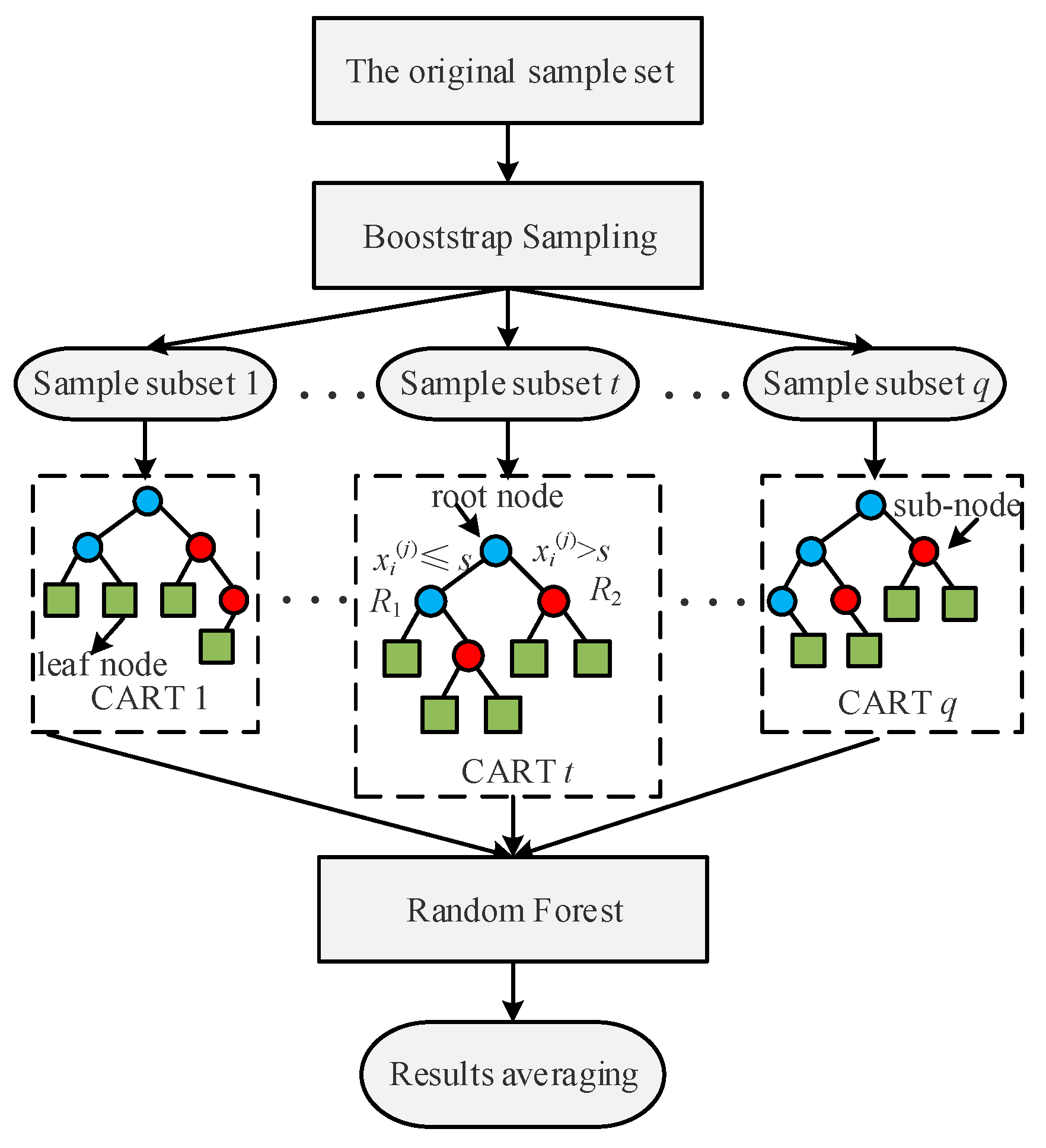
2.1. Random Forest Regression Method

The random forest regression (RFR) method is an integrated regression algorithm based on the classification and regression tree (CART) model [19]. It is well suited to problems of numerical prediction. The process of constructing an RFR model is shown in Figure 1. The CART is an algorithm that recursively constructs a binary tree, dividing the current sample set into two subsets at each node except the leaf [20]. Suppose D is a subset of samples, and X and Y are the input samples and output variables, respectively, then D = {(x₁, y₁), …,(x_i, y_i), …, (x_N, y_N)}. The application steps of the CART algorithm are as follows.

• Construct a root node containing a subset of all samples.
• Iterate over all features and, for feature j, divide the sample set by the intersection point s. First, the values of all features j in the sample subset are ranked from smallest to largest, and s is the average of the two adjacent values after feature ranking. Optimal sample segmentation is the minimization of the objective squared error. By solving for the minimum of Equation (1), the optimal feature and optimal cut-off point of the segmented sample set is obtained.

$$\underset{j,s}{\underbrace{min}}\left[\underset{c_1}{\underbrace{min}}{\displaystyle \sum _{x_i\in R_1(j,s)}{(y_i-c_i)}^2+\underset{c_2}{\underbrace{min}}{\displaystyle \sum _{x_i\in R_2(j,s)}{(y_i-c_i)}^2}}\right]$$

(1)

where R₁ and R₂ are the two subspace units divided according to the cut-off point s.

$$R_1(j,s)=\left\{x_i\right|x_i^{(j)}\le s\}$$

$$R_2(j,s)=\left\{x_i\right|x_i^{(j)}>s\}$$

where i = 1, 2, …, N, and j = 1, 2, …, f, c₁, c₂ are the mean values of the output variable Y on subspace cells R₁ and R_2, respectively.

3.

Continue to repeat step 1 and step 2 for the 2 subunits until the entire decision tree is grown and all samples in the subset are assigned to the leaf nodes. The prediction result corresponds to y_i is [21]

$${\widehat{y}}_i=\frac{1}{K}{\displaystyle \sum _{k=1}^K{\widehat{T}}_k\left(x_i\right)}$$

where K is the number of decision tree, and ${\widehat{T}}_k(x_i)$ denotes the estimation results produced by the k-th tree.

The RFR model uses bagging sampling to randomly select samples in a put-back fashion. Then q variables (q < m, m is the number of features) are randomly selected at each node and used as candidates for splitting the node to construct a single decision tree. The above steps are repeated to generate a large number of regression decision trees. The final prediction result of the model is the average of the prediction results of several CART models.

2.2. TPE-XGBoost Method

The extreme gradient boosting (XGBoost) algorithm uses CART as the base classifier and integrates it with gradient boosting [22]. The gradient boosting framework of the XGBoost model makes it more efficient and flexible [23]. Compared with the Gradient Boosting Decision Tree algorithm, the generalization capability of XGBoost is improved by using advanced regularization. The basic principle is that each time a new CART is added as a base evaluator, the prediction residuals of the previous CART are fitted. The prediction results of all CARTs are accumulated to obtain the final results of the model. At the same time, the XGBoost algorithm adds a regularization term to the loss function, which greatly reduces the model complexity and can achieve a balance between model accuracy and complexity. Suppose the feature dimension of the sample data is m, and the training dataset S = {(x₁,y₁), …, (x_n,y_n)} includes n samples, where x_i = (x_i1, …, x_im). If the XGBoost model contains t weak evaluators, then the classification result of sample x_i is

$$y_i^t={\displaystyle \sum _{k=1}^t{f}_k(x_i),f_k\in F}$$

where y_i denotes the diagnostic result of sample x_i, f_k denotes the k-th weak evaluator, and F denotes the function space containing every potential regression tree. The objective function L of the XGBoost model is

$$L^{(t)}={\displaystyle \sum _{i=1}^{n}l(y_i,y_i^{(t-1)}+f_t(x_i))+\mathsf{\Omega }(f_t)}$$

where l is the loss function, which represents the difference between the classification result and the real value; Ω is the regularization term, which is used to reduce the risk of overfitting in the classification process, and the expression is

$$\mathsf{\Omega }(f_k)=\gamma T+\frac{1}{2}\lambda {\displaystyle \sum _{j=1}^T{\omega }_j^2}$$

where γ and λ are the parameters used to prevent overfitting, T is the number of nodes, and ω denotes the weight of each node.

The objective function after the second-order Taylor series expansion is

$$L^{(t)}\approx {\displaystyle \sum _{i=1}^n\left[l(y_i^{t-1},y_i)+g_i{f}_t(x_i)+\frac{1}{2}{h}_i{f}_t^2(x_i)\right]}+\mathsf{\Omega }(f_t)$$

where g_i and h_i are the first- and second-order derivatives, respectively, and the expressions are

$$g_i={\partial }_{y_i^{(t-1)}}l(y_i^{(t-1)},y_i)$$

$$h_i={\partial }_{y_i^{(t-1)}}^{2}l(y_i^{(t-1)},y_i)$$

Further, by removing the constant term of the objective function, then

$$L^{(t)}\approx {\displaystyle \sum _{i=1}^n\left[g_i{f}_t(x_i)+\frac{1}{2}{h}_i{f}_t^2(x_i)\right]}+\mathsf{\Omega }(f_t)$$

(2)

If the dataset of sample numbers in leaf node j is defined as

$$I_j=\left\{i\right|q(x_i)=j\}$$

where q(x_i) is the value of the leaf label corresponding to x_i. Then, the solution of Equation (2) is

$$w_j^{\ast }=-\frac{{\displaystyle \sum _{i\in I_j}{g}_j}}{{\displaystyle \sum _{i\in h_j}{h}_j}+\lambda }$$

$$f_{obj}=-\frac{1}{2}{\displaystyle \sum _{j=1}^T\left(\frac{{\displaystyle \sum _{i\in I_j}{g}_j}}{{\displaystyle \sum _{i\in h_j}{h}_j}+\lambda }\right)+\gamma T}$$

2.3. TPE Optimization Method

The Bayesian optimization algorithm uses a probabilistic proxy model to fit the objective function. It selects the next evaluation point based on the results of the prior sampling, thus quickly finding the optional value [24].

$$p(f|H_i)=\frac{p(H_i|f)p(f)}{p(H_i)}$$

(3)

$$H_i=\left\{\left(x_1,f(x_1)\right),\dots ,\left(x_i,f(x_i)\right)\right\}$$

where p(f) and p(H_i|f) are the prior and likelihood distributions of f, respectively, and p(f|H_i) is the posterior probability distribution.

In order to solve the problems of the large parameter space and the complexity of parameter tuning of the XGBoost model, the tree-structured Parzen estimator (TPE) algorithm is adopted as the probability estimation for sampling points of parameter intervals [25]. The probability distribution p(H_i|f) in Equation (3) is defined as

$$p(x|y)=\left\{\begin{array}{l}l(x), y<y^{\ast }\\ g(x), y\ge y^{\ast } \end{array}\right.$$

where y* = min{(x₁,f(x₁)), …, (x_i,f(x_i))}, denotes the optimal sampling threshold; l(x) and g(x) are the probability estimates of p(x|y) in the loss function of observation x. The expected value of the sampling function is

$$E_{y^{\ast }}(x)={\displaystyle {\int }_{-\infty }^{y^{\ast }}(y^{\ast }-y)\frac{p(x|y)p(y)}{p(x)}dy}$$

If γ = p(y < y*), and p(x) is equal to

$$p(x)=g(x)\gamma l(x)-(1-\gamma )$$

$${\displaystyle {\int }_{-\infty }^{y^{\ast }}(y^{\ast }-y)p(x|y)p(y)dy}=\gamma y^{\ast }l(x)-l(x){\displaystyle {\int }_{-\infty }^{y^{\ast }}p(y)dy}$$

then the expected value is converted to

$$E_{y^{\ast }}(x)=\frac{\gamma y^{\ast }l(x)-l(x){\displaystyle {\int }_{-\infty }^{y^{\ast }}p(y)dy}}{\gamma l(x)-(1-\gamma )g(x)}$$

When the conditions that l(x) is the maximum and g(x) is the minimum are satisfied at the same time, the expected value is maximum, and the corresponding sampling point x is obtained.

3. Transformer Fault Diagnosis Method

The transformer fault diagnosis method proposed in the article includes the following three processes: a missing data-filling model based on the RFR method, hyperparameter optimization based on TPE, and a fault diagnosis model based on the TPE-XGBoost method.

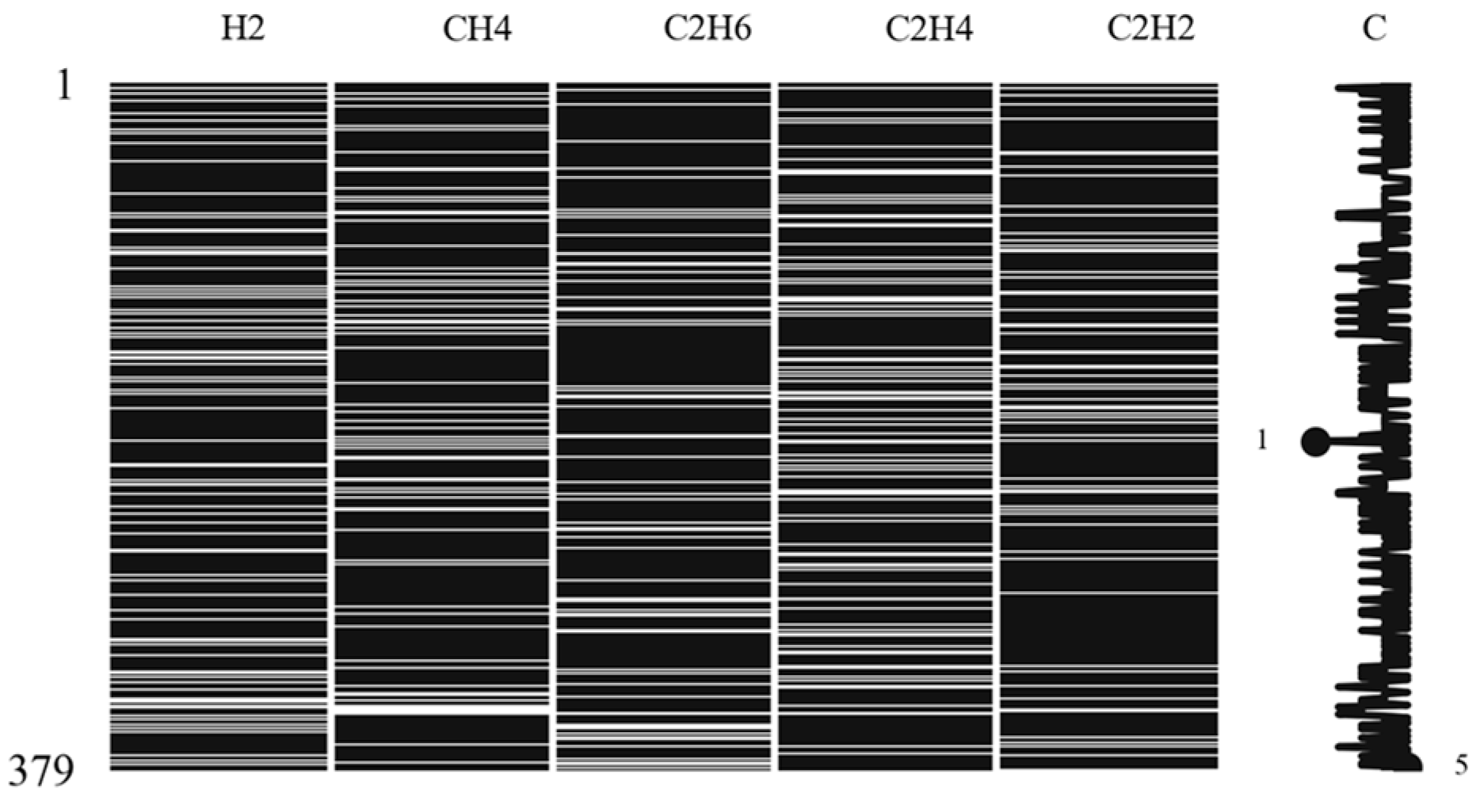
3.1. DGA Sample Dataset

When a discharge or overheating fault occurs inside the power transformer, the transformer oil pyrolyzes, producing hydrogen (H₂), methane (CH₄) and other hydrocarbon gases [26]. According to IEC 60599 [11], transformer fault diagnosis results based on DGA are mainly classified into normal status (N), thermal faults and electrical faults. Distinguished by the severity of the fault, overheating faults can be divided into T1 (t < 300 °C), T2 (300 °C < t < 700 °C) and T3 (t > 700 °C), and electrical faults include PD (corona partial discharges), D1 (discharges of low energy) and D2 (discharges of high energy). Three hundred and seventy-nine transformer failure cases were collected from a DGA sample dataset, of which the sample distribution is shown in Figure 2.

The abnormal values in the DGA samples have a great impact on the fault diagnosis results. The statistical analysis of the DGA sample data is shown in

Table 1. Statistics Analysis of DGA Samples.

Value	H2	CH4	C2H6	C2H4	C2H2
mean	222.38	122.25	73.14	164.26	29.00
standard	453.83	298.97	281.79	359.65	76.18
minimum	0	0	0	0	0
1st quartile	18.50	10.90	2.48	2.60	0
2nd quartile	72.20	43.00	17.80	30.00	0.30
3rd quartile	191.46	136.60	54.00	147.05	13.75
maximum	3433.00	4992.00	4836.00	3671.00	765.20

.

The differences in the mean, standard and even maximum values of the different gas contents in the samples are significant. In order to reduce the influence of numerical differences on the diagnosis results, the paper normalized the gas content by (4).

$$x_{ij}^{\ast }=\frac{x_{ij}}{{\displaystyle \sum _{k=1}^5{x}_{ik}}}$$

(4)

where x_ij is the j-th gas content in the i-th DGA sample.

In order to improve the accuracy of transformer diagnostic results, this paper performs feature derivation of DGA gases. The five gas contents of H₂, CH₄, C₂H₆, C₂H₄ and C₂H₂ are expanded to 16 features, as shown in

Table 2. Derivation results of DGA features.

No.	Features	No.	Features
1	M(H2)	9	C(C2H4/C2H6)
2	M(CH4)	10	K(H2/(H2 + TH))
3	M(C2H6)	11	K(C2H4/TH)
4	M(C2H4)	12	K(C2H6/TH)
5	M(C2H2)	13	K(C2H2/TH)
6	M(TH)	14	K((CH4 + C2H4)/TH)
7	C(C2H2/C2H4)	15	K((C2H4 + C2H6)/TH)
8	C(CH4/H2)	16	K((C2H2 + CH4)/TH)

. The features derived in this paper mainly include three categories: gas content, three basic gas ratios and other gas ratios [11]. Among them, TH represents total hydrocarbon, M(·) represents gas content, C(·) represents three gas ratios, and K(·) represents other gas ratios adopted.

3.2. Missing Data Filling Method

In order to verify the filling effect of the RFR algorithm on incomplete data, the sample values are artificially and randomly removed. The distribution of 20% missing values in the sample data is shown in Figure 3. The black part represents that the feature value is available, while the white part represents missing data. The larger the white areas in the graph, the less complete the feature. The C represents the integrity of the data.

For continuous features, zero or mean value is often used to replace missing values in the sample data. However, given the intrinsic relationship between dissolved gases in oil, the regression algorithm is able to learn from the sample data to achieve prediction and filling of missing values.

The main process of numerical filling using the RFR model is as follows:

• Analyze missing sample data and construct a sample set based on missing values and treat-filled features as labels.
• Select the sample data with the least number of missing values for filling-in priority. The missing values of features other than the feature to be filled are temporarily replaced by their mean.
• Predict the values of the missing data using RFR and insert the predicted results into the original sample set.
• Repeat steps 1–3 until the last feature with the highest number of missing values is predicted by a final regression on it using the original sample after filling.

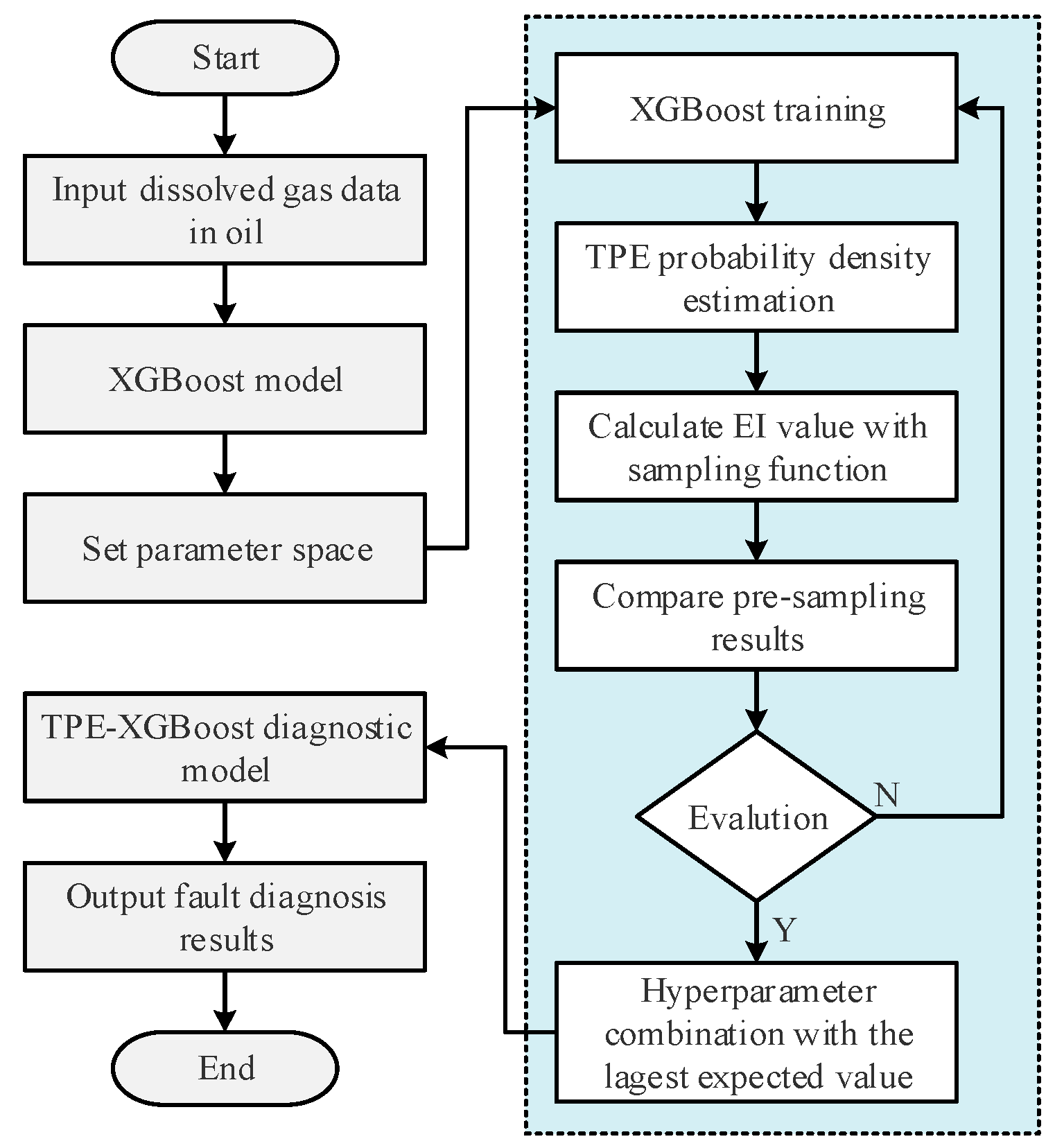
3.3. Transformer Fault Diagnosis Model

The TPE method is introduced into the transformer fault diagnosis model to overcome the shortcomings of cross-validation and grid search methods. The model accuracy is improved by simultaneous optimization of multiple hyperparameters of XGBoost.

The main parameters of the XGBoost method include Booster, General and Learning parameters [22]. The values of the different parameters directly affect the diagnostic effect of the model. Traditional parameter searching methods rely on experience or parameter traversal, while the Gaussian mixture-based TPE method has a sparser parameter space and is more efficient in parameter search. The parameters that have a greater impact on the XGBoost model are selected for searching, as shown in

Table 3. XGBoost Parameters.

Parameter	Range	Step Size	Parameter	Range	Step Size
num_boost_round	[20, 300]	1	eta	[0.1, 1]	0.05
colsamble_by_tree	[0.3, 1]	0.05	booster	[‘gbtree’, ‘dart’]	/
colsample_by_node	[0.1, 1]	0.05	gamma	[0.5, 2]	0.1
min_child_weight	[0, 5]	0.05	lambda	[0, 3]	0.1
max_depth	[2, 30]	1	subsamples	[0.1, 1]	0.05

.

The process of the TPE-XGBoost transformer fault diagnosis model proposed in this paper is shown in Figure 4. The application steps are as follows:

• Input dissolved gas data in oil to construct an XGBoost model and set XGBoost parameter ranges.
• Train the XGBoost model and perform TPE probability density estimation. The expected value is calculated by the sampling function, and the next combination of parameters to be evaluated is selected based on the prior expected value.
• Use the combination of parameters with the maximum expected value in the XGBoost model for training to output the prediction results of the model with the current hyperparameters.
• If the error of the newly selected parameter combination meets the requirements, the algorithm will be terminated, and the corresponding parameter combination and model prediction error will be output. If not, the sampling function will be corrected and go back to step (2) until the set requirement is met.
• According to the optimal parameters of XGBoost, the final fault diagnosis model based on TPE-XGBoost is obtained, and the fault diagnosis results are output.

4. Application Results and Analysis

The 379 DGA data shown in Figure 2 constitute the sample database of this paper and are divided into training and test samples in the ratio of 7:3. After the process of missing data filling, TPE parameter optimization and model training, the effects of fault diagnosis methods on the diagnosis results are analyzed and discussed.

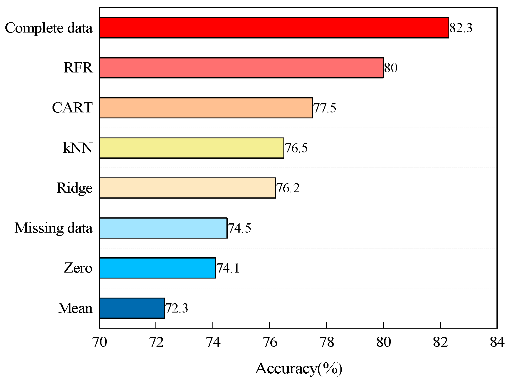
4.1. Analysis of Data Filling Methods

The effectiveness of the method for filling in missing data in DGA samples should be based on the accuracy of the diagnostic results. Therefore, this paper combines statistical methods, kNN [27], ridge regression (Ridge) [28], CART and RFR to analyze the diagnostic results, as shown in Figure 5.

The diagnostic accuracy of the XGBoost model with complete data is 82.3%. The results show that RFR and CART methods are better than kNN, Ridge and statistical methods at filling in the missing values of DGA data, which indicates that the relationship between DGA characteristic gases is non-linear. In addition, the accuracy of the diagnostic results is 74.5% when the missing data are not treated in any way. The accuracy is slightly reduced when missing values are filled in using zero or mean values. Compared to the missing data, the diagnostic effect of the data filled by the RFR method is improved by 5.5%, and its accuracy rate reaches 80%, indicating that the RFR method can effectively restore the information of missing data in DGA samples.

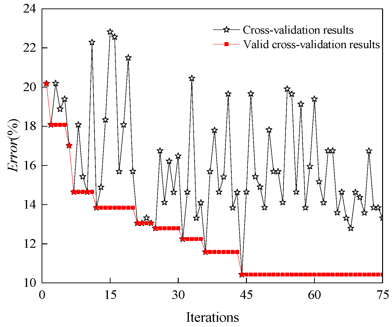
4.2. Parameter Optimization of XGBoost Model

As the TPE optimization algorithm only supports searching for the minimum of the objective function, the evaluation metric error is chosen as the objective function for parameter searching. The formula for error is as follows.

$$E(f;S)=\frac{1}{n}{\displaystyle \sum _{i=1}^{n}f(y_i\ne {y^{\prime }}_i)}$$

where n is the number of samples, S is the training samples, y_i denotes the true category of sample x_i, and f(x_i) denotes the prediction category.

The iterative process of TPE optimization is shown in Figure 6. The TPE algorithm finds valid sampling points by randomly sampling the XGBoost parameter space and performing a cross-validation calculation under the training set. When the number of iterations is 44, the minimum error value of 10.43% is obtained. There is no decline for 30 iterations; thus, the TPE algorithm optimization iteration is terminated.

Compared to the diagnostic results of XGBoost in Figure 5, the accuracy of the TPE-XGBoost diagnostic model after parameter tuning is close to 90%. The optimal combination of parameters for the TPE-XGBoost diagnostic model is shown in

Table 4. Optimal parameters by TPE algorithm.

Parameter	Value	Parameter	Value
num_boost_round	239	eta	0.15
colsamble_by_tree	0.80	booster	‘gbtree’
colsample_by_node	0.20	gamma	1.20
min_child_weight	1.20	lambda	3.10
max_depth	4	subsamples	1

.

4.3. Analysis of Fault Diagnosis Methods

The confusion matrix can be used to visualize the results of the diagnostic model for different fault types. Based on the 114 test set samples after the RFR model fills in the missing data, the diagnostic results of the XGBoost model and TPE-XGBoost model are shown in Figure 7 and Figure 8. The results show that the diagnostic accuracy of the XGBoost model and the TPE-XGBoost model is 84.2% and 89.5%, respectively. The accuracy of the fault diagnosis model increased significantly with TPE optimization.

The TPE-XGBoost diagnostic model is noticeably improved in terms of T2 and varying degrees of discharge faults. Discharges of high energy are particularly diagnosed with an accuracy of 95%. Each fault type is diagonally distributed along the confusion matrix, indicating that the TPE-XGBoost model has excellent diagnostic effects on the test set.

Three evaluation metrics, F1-score, precision and recall, are used to further evaluate the merits of the model for different fault types in this paper, as shown in Figure 9. Precision is the percentage of positive tuples predicted to be identified by the model; recall indicates the percentage of positive tuples correctly identified by the model; F1-score is the harmonic mean of precision and recall. The closer the three evaluation indicators above are to 1, the better the diagnostic performance of the model.

The results show that all merits of the TPE-XGBoost model are higher than 0.7, and most of them are higher than 0.82. Of these, the three evaluation indicators corresponding to normal and discharges of high energy are over 0.90. Combining the seven diagnostic results, the average value of the F1 score is 0.87, which verifies the excellent stability and robustness of TPE-XGBoost in transformer fault diagnosis.

4.4. Discussion

Based on the DGA dataset with a missing data rate of 20%, the TPE-XGBoost method is compared with other methods, including kNN, RF, CART, Natural Gradient Boosting (NGBoost) and 100-layer deep neural networks (DNN) [29]. The accuracy of each model is evaluated by the five-fold cross-validation method, as shown in Figure 10. The yellow line in the box diagram indicates the median of diagnostic result.

The performance of the TPE-XGBoost method is better than other algorithms, with an average accuracy of 89.5%. The diagnostic accuracy of the linear classification algorithm is lower than that of the other non-linear models. The kNN method is prone to misjudgment between different fault types corresponding to the same fault properties, especially for partial discharge and low energy discharge faults. This may be caused by the non-linear relationship between the DGA data and the energy of the transformer fault. In addition, the performance of integrated algorithms, such as RF and XGBoost, is much better than single models, such as CART and DNN. The accuracy of the NGBoost algorithm is higher than the XGBoost algorithm but slightly lower than the TPE-XGBoost algorithm. However, according to the results of multiple cross-validations, the robustness of the XGBoost and NGBoost models is worse than that of the TPE-XGBoost models, indicating that the TPE algorithm improves the accuracy and robustness of the fault diagnosis models effectively.

Subsequently, the statistical differences in the diagnosis accuracy of the above methods are analyzed by a one-sample t-test [30]. Considering that the IEC Three Ratio method has a diagnostic accuracy of 86.0% in the case of complete data, the null hypothesis is that the accuracy of the diagnostic model is equal to 86.0%. The results are shown in

Table 5. Statistical test results of different methods.

Method	Sample Size	Minimum	Maximum	Mean	Standard Deviation	t Value	p Value
kNN	10	0.661	0.857	0.772	0.062	−4.495	0.001
CART	10	0.694	0.861	0.779	0.057	−4.46	0.002
DNN	10	0.639	0.917	0.792	0.097	−2.231	0.053
RF	10	0.75	0.895	0.834	0.049	−1.68	0.127
XGBoost	10	0.767	0.943	0.861	0.056	0.048	0.963
NGBoost	10	0.768	0.956	0.877	0.063	0.852	0.417
TPE-XGBoost	10	0.837	0.955	0.9	0.037	3.374	0.008

.

The results show that for kNN, CART and TPE-XGBoost methods, the null hypothesis is clearly rejected based on the test with a 95% confidence level. According to the t and p values of the above three methods, the accuracy of the TPE-XGBoost algorithm is significantly higher than 86%, while the other two are lower than 86%. This also shows that the method proposed in this paper has a significant improvement in dealing with the fault diagnosis problem of incomplete DGA data.

Lastly, the diagnostic accuracy of the TPE-XGBoost model with different data missing rates were analyzed and discussed, as shown in Figure 11. The results show that the data missing rate has a significant impact on the diagnostic accuracy of the model. However, when the data missing rate is greater than 20%, the decreased rate of accuracy is significantly accelerated. When the data missing rate is below 30%, the diagnostic accuracy of the model is below 80%. This indicates that the method proposed in the paper still has limitations in dealing with cases of a high missing rate, such as more than 30%, and its diagnostic result still needs to be improved.

5. Conclusions

A transformer fault diagnosis model based on RFR and TPE-XGBoost algorithms which is able to handle incomplete datasets, is proposed in this paper. First, the RFR algorithm was used to fill in the missing values in the sample data and compare them with statistical methods and other data-filling methods. Then, the TPE method was used to optimize the XGBoost model and improve the accuracy of the fault diagnosis model. Finally, the accuracy of TPE-XGBoost was compared with other artificial intelligence algorithms to verify its effectiveness. The conclusions of this paper are as follows.

• The RFR algorithm outperformed traditional statistical methods and CART, kNN, and Ridge for the missing data problem of dissolved gas in transformer oil. The accuracy of the RFR model reached 80% when the missing rate of DGA data was 20%, indicating that the RFR-filled values could restore the information of the dissolved gas in the transformer oil to a greater extent.
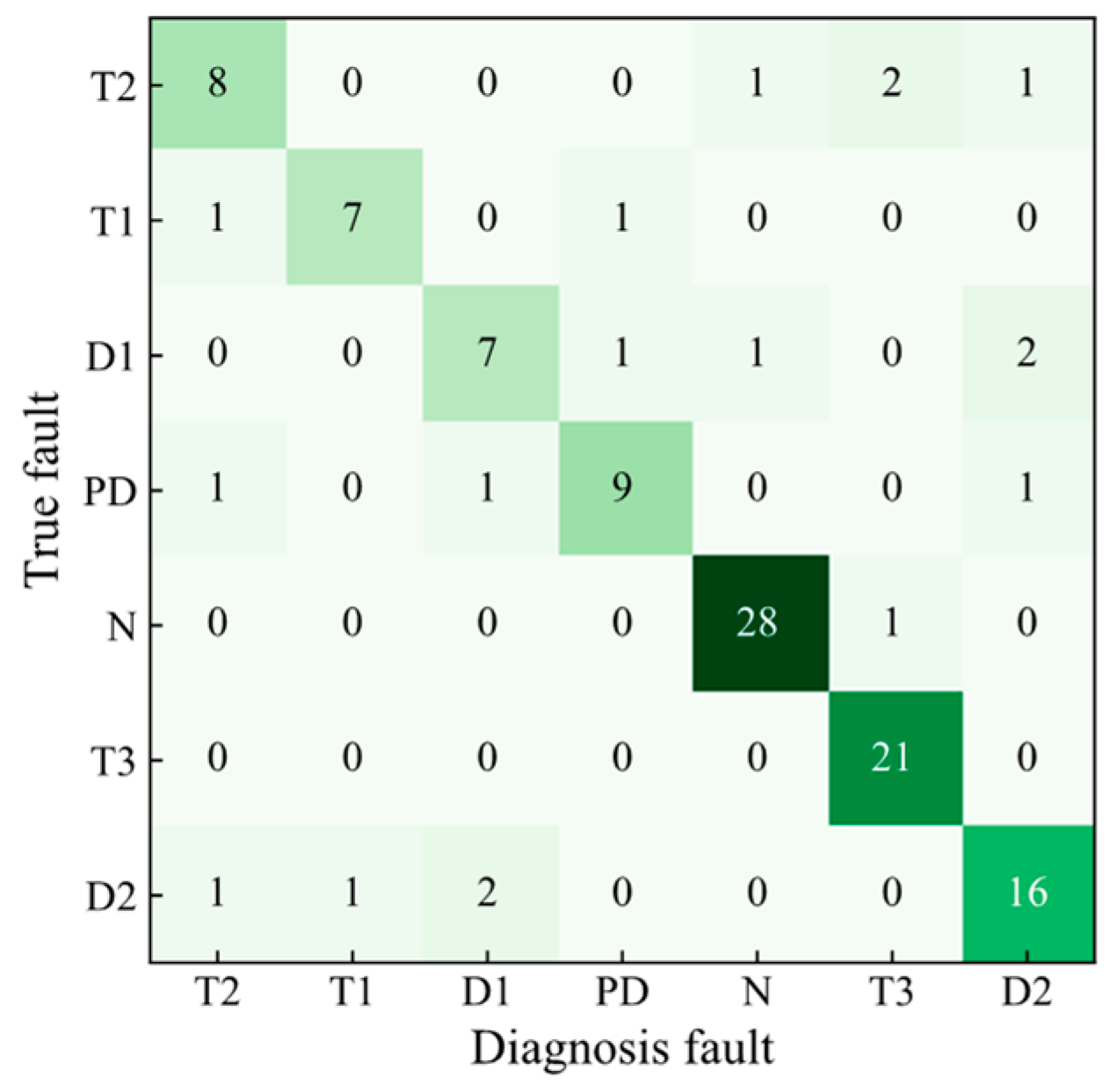
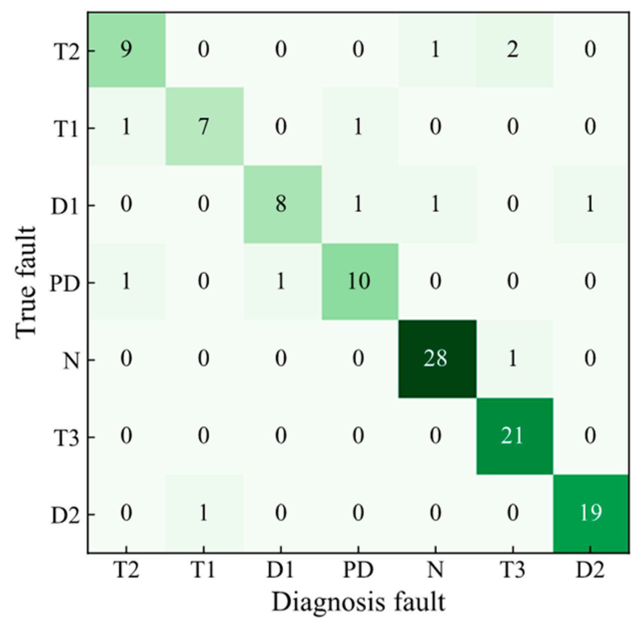
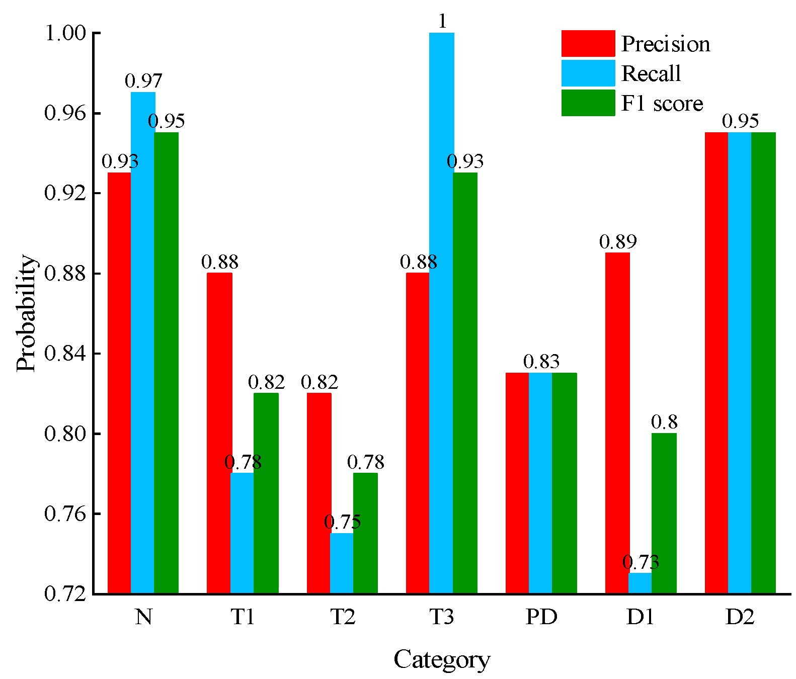
• Based on the DGA sample database, after the RFR model fills in the missing data, the accuracy of the XGBoost model was improved from 80% to 89.5% after feature derivation and hyper-parameter optimization of the TPE algorithm. The evaluation metric F1-score of the TPE-XGBoost model was 87%, indicating the effectiveness of the TPE-XGBoost diagnostic model.
• The TPE-XGBoost algorithm was compared with kNN, CART, RF and DNN. Based on the DGA sample dataset with 20% missing values, the average accuracy of the TPE-XGBoost model was 89.5% and was much higher than the other algorithms. The superiority of the TPE-XGBoost algorithm in dealing with transformer fault diagnosis problems was demonstrated. The diagnosis results obtained in the case of partially missing data were still credible.

References

1. Ghoneim, S.S.M.; Mahmoud, K.; Lehtonen, M.; Darwish, M.F. Enhancing diagnostic accuracy of transformer faults using teaching-learning-based optimization. IEEE Access 2021, 9, 30817–30832. [Google Scholar] [CrossRef]
2. Rao, U.M.; Fofana, I.; Rajesh, K.N.V.P.S.; Picher, P. Identification and application of machine learning algorithms for transformer dissolved gas analysis. IEEE Trans. Dielect. Electr. Insul. 2021, 28, 1828–1835. [Google Scholar] [CrossRef]
3. Kahlen, J.N.; Andres, M.; Moser, A. Improving machine-learning diagnostics with model-based data augmentation showcased for a transformer fault. Energies 2021, 14, 6816. [Google Scholar] [CrossRef]
4. Tang, L.R.; Wang, R.; Wu, R.; Fan, B. Missing data filling algorithm for uniform data model in panoramic dispatching and control system. Autom. Electr. Power Syst. 2017, 41, 25–30+87. [Google Scholar]
5. Santos, M.S.; Pereira, R.C.; Costa, A.F.; Soares, J.P.; Santos, J.; Abreu, P.H. Generating synthetic missing data: A review by missing mechanism. IEEE Access 2019, 7, 11651–11667. [Google Scholar] [CrossRef]
6. Cheng, X.; Li, P.; Guo, L.; Zhang, W. Transformer operating state monitoring method based on Bayesian probability matrix decomposition of measurement data. Proc. CSU-EPSA 2022, 34, 100–107. [Google Scholar]
7. Wu, L.Z.; Zhu, Y.L.; Yuan, J.H. Novel method for transformer faults integrated diagnosis based on Bayesian network classifier. Trans. China Electrotech. Soc. 2005, 20, 45–51. [Google Scholar]
8. Roger, R.R. IEEE and IEC Codes to interpret incipient faults in transformers, using gas in oil analysis. IEEE Trans. Dielect. Electr. Insul. 1978, 13, 349–354. [Google Scholar] [CrossRef]
9. Duval, M. Dissolved Gas Analysis: It Can Save Your Transformer. IEEE Electr. Insul. Mag. 1989, 5, 22–27. [Google Scholar] [CrossRef]
10. Dornenburg, E.; Strittmatter, W. Monitoring oil-cooled transformers by gas analysis. Brown Boveri Rev. 1974, 61, 238–247. [Google Scholar]
11. Duval, M.; Depabla, A. Interpretation of gas-in-oil analysis using new IEC publication 60599 and IEC TC 10 databases. IEEE Electr. Insul. Mag. 2001, 17, 31–41. [Google Scholar] [CrossRef]
12. Duval, M.; Lamarre, L. The Duval Pentagon—A new complementary tool for the interpretation of dissolved gas analysis in transformers. IEEE Electr. Insul. Mag. 2014, 30, 9–12. [Google Scholar]
13. Taha, I.B.M.; Ghoneim, S.S.M.; Duaywah, A.S.A. Refining DGA methods of IEC code and rogers four ratios for transformer fault diagnosis. IEEE Power Energy Soc. Gen. Meet. 2016, 2016, 7741157. [Google Scholar]
14. Tightiz, L.; Nasab, M.; Yang, H.; Addeh, A. An intelligent system based on optimized ANFIS and association rules for power transformer fault diagnosis. ISA Trans. 2020, 103, 63–74. [Google Scholar] [CrossRef]
15. Bacha, K.; Souahlia, S.; Gossa, M. Power transformer fault diagnosis based on dissolved gas analysis by support vector machine. Electr. Power Syst. Res. 2012, 83, 73–79. [Google Scholar] [CrossRef]
16. Pei, X.; Zheng, X.; Wu, J. Rotating Machinery Fault Diagnosis Through a Transformer Convolution Network Subjected to Transfer Learning. IEEE Trans. Instrum. Meas. 2021, 70, 2515611. [Google Scholar] [CrossRef]
17. Haque, N.; Jamshed, A.; Chatterjee, K.; Chatterjee, S. Accurate Sensing of Power Transformer Faults from Dissolved Gas Data Using Random Forest Classifier Aided by Data Clustering Method. IEEE Sens. J. 2022, 22, 5902–5910. [Google Scholar] [CrossRef]
18. Das, S.; Paramane, A.; Chatterjee, S.; Rao, U.M. Accurate Identification of Transformer Faults from Dissolved Gas Data Using Recursive Feature Elimination Method. IEEE Trans. Dielectr. Electr. Insul. 2023, 30, 466–473. [Google Scholar] [CrossRef]
19. Breiman, L. Random forests. Mach. Learn. 2001, 45, 5–32. [Google Scholar] [CrossRef] [Green Version]
20. Breiman, L. Classification and Regression Trees; Wadsworth International Group: Belmont, CA, USA, 1984. [Google Scholar]
21. Chehreh, S.C.; Nasiri, H.; Tohry, A. Modeling industrial hydrocyclone operational variables by SHAP-CatBoost—A “conscious lab” approach. Powder Technol. 2023, 420, 118416. [Google Scholar] [CrossRef]
22. Chen, T.; Guestrin, C. XGBoost: A scalable tree boosting system. In Proceedings of the 22nd ACM SIGKDD International Conference on Knowledge Discovery and Data Mining (KDD), San Francisco, CA, USA, 13–17 August 2016; pp. 785–794. [Google Scholar]
23. Fatahi, R.; Nasiri, H.; Homafar, A. Modeling operational cement rotary kiln variables with explainable artificial intelligence methods—A “conscious lab” development. Part. Sci. Technol. 2023, 40, 715–724. [Google Scholar] [CrossRef]
24. Shahriari, B.; Swersky, K.; Wang, Z.; Adams, R.P.; Freitas, N.D. Taking the human out of the loop: A review of Bayesian optimization. Proc. IEEE 2016, 104, 148–175. [Google Scholar] [CrossRef] [Green Version]
25. Bardenet, B.R.; Bengio, Y.; Kégl, B. Algorithms for hyperparameter optimization. Proc. Adv. Neural Inf. Process. Syst. 2011, 24, 1–9. [Google Scholar]
26. Hoballah, A.; Mansour, D.-E.A.; Taha, I.B.M. Hybrid Grey Wolf Optimizer for Transformer Fault Diagnosis Using Dissolved Gases Considering Uncertainty in Measurements. IEEE Access 2020, 8, 139176–139187. [Google Scholar] [CrossRef]
27. Cover, T.; Hart, P. Nearest neighbor pattern classification. IEEE Trans. Inf. Theory 1967, 13, 21–27. [Google Scholar] [CrossRef] [Green Version]
28. Ozkale, M.R.; Lemeshow, S.; Sturdivant, R. Logistic regression diagnostics in ridge regression. Comput. Stat. 2018, 33, 563–593. [Google Scholar] [CrossRef]
29. Xu, X.; Li, Y.; Yuan, C. Identity bracelets for feep neural networks. IEEE Access 2020, 8, 102065–102074. [Google Scholar] [CrossRef]
30. Nasiri, H.; Ebadzadeh, M.M. MFRFNN: Multi-functional recurrent fuzzy neural network for chaotic time series prediction. Neurocomputing 2022, 507, 292–310. [Google Scholar] [CrossRef]
Figure 1. The structure diagram of RFR model.
Applsci 13 07539 g001
Figure 2. Distribution of transformer fault samples.
Applsci 13 07539 g002
Figure 3. Distribution of missing values in the sample dataset.
Applsci 13 07539 g003
Figure 4. Flowchart fault diagnosis model based on TPE-XGBoost.
Applsci 13 07539 g004
Figure 5. Comparison of the effect of filling methods on diagnostic results.
Applsci 13 07539 g005
Figure 6. TPE optimization iteration process.
Applsci 13 07539 g006
Figure 7. Confusion matrix of XGBoost model.
Applsci 13 07539 g007
Figure 8. Confusion matrix of TPE-XGBoost model.
Applsci 13 07539 g008
Figure 9. Evaluation metrics for TPE-XGBoost diagnostic model.
Applsci 13 07539 g009
Figure 10. Comparison of the accuracy of different diagnostic models.
Applsci 13 07539 g010
Figure 11. The influence of data missing rate on diagnostic result.
Applsci 13 07539 g011