Competing Failure Modeling for Systems under Classified Random Shocks and Degradation

Abstract

A new model is presented to analyze reliability for systems subjected to competing risks of a typical degradation process and external random shocks. The external random shocks may cause hard failure and instantaneous increases in the degradation process. Random shocks are classified into three types in the new model according to their sizes. Different types will lead to different instantaneous increases in the degradation process. Besides system reliability, the competing failure probabilities are also studied. Competing failure probability indicates the probability that one risk mode fails while the other risk mode does not fail. Competing failure probabilities are helpful in determining which risk mode is more likely to occur during a system’s lifetime. It is impractical if both risk modes fail together for systems under competing failure modes, while the system reliability and failure probabilities, which are simply calculated by expression, do not resolve this impractical situation. The modified values of system reliability and competing failure probability are calculated in this paper with the impractical situation excluded. The effectiveness of the presented model is demonstrated by the reliability analysis of the micro-electromechanical system (MEMS), which proved that the probabilities calculated using this method are more practical. In addition, sensitivity analysis is performed for specific parameters.

1. Introduction

Generally, systems are exposed to external random shocks and under internal wastage during their working time. Wear or tribology are the most typical forms of wastage for mechanical systems. Either applied random shocks or internal wastage may lead to the failure of a system, specifically, the shock risk mode (hard failure mode) and degradation risk mode (soft failure mode). These two risk modes compete with each other, and whichever occurs first may cause the system to fail. It is impossible for both risk modes to occur together due to this competitiveness [1]. To analyze the reliabilities for this type of system, it is of vital importance to model both risk modes and the competing relationship.

There are five classic random shock models.

(1)

The cumulative shock model: This model considers that every shock will cause damage, and as soon as the cumulative damage exceeds the threshold, the hard failure occurs.

(2)

The extreme shock model: Hard failure occurs when the size of any shock exceeds a specific threshold in this model.

(3)

The m-shock model: This model holds that failure occurs when the m-shock sizes are greater than a threshold.

(4)

The run shock model: Similar to the extreme model and the m-shock model, it fails when a run of shocks’ sizes exceeds the threshold.

(5)

The δ shock model: Time lag is selected as the index. Failure occurs when the time lag between two successive shocks is smaller than a threshold.

There are also many research articles concerning random shocks which use the five models. Peng used the extreme shock model to analyze the reliability of systems exposed to external random shock [2]. Rafiee applied the extreme shock model, the δ shock model, and the run shock model in his paper to manage shock problems [3]. Jiang used the extreme shock model, the δ shock model, and the m-shock model to solve random shock problems with shifting thresholds [4]. Rafiee used the extreme shock model to analyze the random shocks with multi-shifting thresholds [5].

There are many models, and copious research has been conducted to target degradation problems. The approaches of the degradation analysis can be divided into three main categories [6]: (1) the general path model, this model uses an appropriate expression with specific parameters to represent the degradation process; (2) the stochastic process model, whereby the Markov process and BM (Brownian motion) are typical stochastic process models to conduct reliability analyses; and (3) the statistical model, this model asks for degradation data to establish the degradation model. Many research papers regarding degradation systems have been conducted. Robin modeled the deterioration of the organic coating layer that protects steel structures from corrosion by three different stochastic processes, Brownian motion, a non-stationary gamma process, and a two-stage hit-and-grow physical process [7]. Si used the degradation path to model the degradation process and estimate reliability, in which a maximum-likelihood parameter estimation method is provided [8]. Xu modeled the degradation process by Brownian motion with drift based on statistics from an accelerated degradation test of accelerometers [9]. The degradation models are widely applied when dealing with degradation problems such as lifetime estimation and maintenance policy-making in practice. Ma estimated the reliability and storage life of FOG (fiber optic gyros) by Brownian motion with drift [10]. Ren predicted the degradation time of a civil aircraft engine by the stochastic process (Brownian motion) [11]. Cai studied the failure process of a sliding rail due to wearing, in which the degradation process is modeled by Brownian motion [12]. As previously mentioned, wear and tribology are the most typical degradation processes for mechanical systems. BAI further studied the wear damage modeling of clearance hinges and the joint failure of motion mechanism in an aerospace vehicle [13]. Haneef studied the motion principle of an internal combustion engine, analyzing and predicting the wear process [14]. However, an ASME Fellow, Professor Norman Jones, stated that repeated impacts might cause the plastic deformation of metal parts, which is more likely to occur than wear failure [15]. The same is true of metal revolute joints, and the performance of the motion mechanism may be influenced. Nandu studied the fracture property of a gear system based on contact and energy release rate. The worn regulation and deformation of the gear were both investigated [16].

Competing risk (failure) models are aimed at analyzing the reliability or failure probability for systems under multi-competing risk modes. The theory of competing risks was developed by demographers and biostatisticians [17]. Ye built a distribution-based reliability model for systems under extreme shocks and natural degradation by the Brown–Proschan model and non-homogeneous Poisson process. Based on this model, the survival probabilities with time can be obtained [18]. Wang established a reliability model for a competing failure system with self-recovery features, based on which a semiconductor laser is studied as an example [19]. The competing risk models are also applied in accelerated tests. Zheng proposed a new estimating procedure for competing risk data with a missing cause of failure [20]. Luo developed a testing methodology based on the reliability target allocation for reliability demonstration under competing failure modes at accelerated conditions. Data from previous research were used to illustrate the methodology [21]. For systems under competing risk modes of external shocks (hard failure) and degradation process (soft failure), David W. Coit conducted a series of research [2,3,4,6,17,18,19]. In reference [2], the reliability and maintenance policy for systems were studied by a fundamental competing risk model. The changing degradation rate and shifting failure thresholds were considered in reference [3] and reference [4] respectively, on the basis of the model in reference [2]. Further, in reference [5], the changing degradation rate and shifting failure thresholds were combined in one model. In reference [22,23] the shocks were separated according to their effects on different components, which led to more definite reliability results. Reference [24] studied maintenance policies for repairable systems under competing failure modes by different shock models.

There are still some insufficiencies in previous models for systems under competing risk modes of external random shocks and degradation processes, especially for mechanical systems under wear and tribology. First, external shocks will cause increments in the degradation process, while the increments are regarded as the same distribution as in the previous paper. However, a shock with a larger size may lead to a larger increment, while a shock with a smaller size may lead to a smaller one. It is inappropriate to use the same distribution for all the increments. Secondly, many previous papers only obtained the system reliability, but the competing failure probability is ignored. The competing failure probability means the probability that one risk mode fails while the other risk mode does not fail. The risk mode with a larger competing failure probability is more dangerous than the other risk mode. The value of competing failure probabilities may change even for an identical system reliability value. Moreover, the competing failure probability for soft failure (soft failure occurs when there is no hard failing) should approach 1, which implies the fact that the system will certainly fail due to wastage when the working time is long enough. However, the results calculated according to previous models do not conform to this fact. Thus, the modified probability value is demonstrated. In this paper, the degradation increments caused by random shocks are classified into three types according to their sizes. The competing failures are also calculated in the presented articles. Meanwhile, the modified probability values are demonstrated.

The remainder of this paper is structured as follows. Section 2 is the description of the system and notation for the whole article. Models for the degradation process risk mode (soft) and external shock risk mode (hard) are established in Section 3. Section 4 deduces the system reliability and failure probability based on a model in Section 3. Meanwhile, the modified probabilities for system reliability and failure probabilities are presented. The failure analysis and reliability calculation of a micro-engine is studied as a numerical case, illustrating the model in Section 5. Finally, conclusions and summaries are in Section 6.

2. System Description and Notation

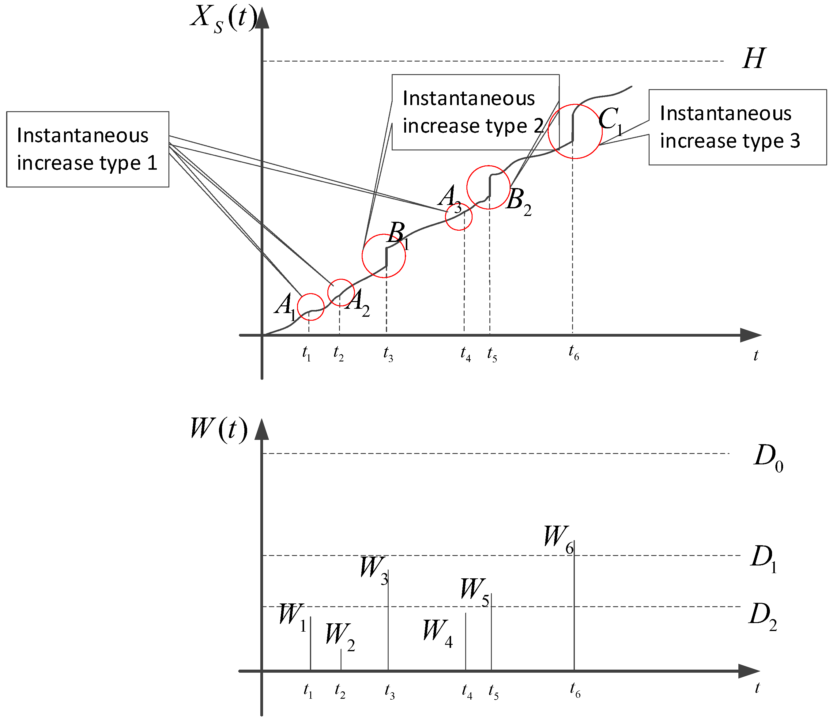
2.1. System Description

Generally speaking, competing failure modes for the system consists of soft failure (degradation risk mode) and hard failure (shock risk mode). As shown in Figure 1, there are two failure processes for a system, the soft failure and the hard failure. Soft failure occurs when the total degradation exceeds its threshold. Hard failure occurs when a random shock magnitude is greater than the threshold value. These two processes compete with each other, which means that whichever failure occurs first, the system will be disrupted.

For hard failure, once an external shock exceeds the failure threshold D₀, hard failure occurs. The appearance of external shocks follows a Poisson process with rate λ. In addition, the sizes of shocks are random variables $W_i$ with specific distribution, so the probability of hard failure has great relation to the $W_i$.

For soft failure, total degradation is composed of pure degradation due to regular wastage (such as wear, aging, and fatigue) and instantaneous increases caused by random shocks. The magnitudes of increases are related to the shock sizes. Three kinds of instantaneous increases for degradation are taken into consideration in this paper, as shown in Figure 1. If the size of one shock is less than a given degradation increase threshold D₂, the increase would be type A_i, or more specifically, no increase. If the size of one shock is between the given thresholds D₁ and D₂, the increase would be type B_j, which is a random variable. Similarly, the increases would be type C_k if the size of one shock is greater than the given condition D₁.

The system is under competing risk modes and will stay valid if neither hard failure nor soft failure occurs. No matter which risk mode (hard failure or soft failure) occurs first, the system fails, and then the other risk mode will not occur anymore.

2.2. Notation

$X_s\left(t\right)$	Overall degradation
$X\left(t\right)$	Pure degradation
$S\left(t\right)$	Degradation increment caused by external random shocks
Wi	Size of the ith random shock
Ai  Bj  Ck	Three types of degradation increments, which are i.i.d. random variables
rn	Rate of shock type n
$N_n\left(t\right){\lambda }_n$	Poisson process n with rate ${\lambda }_n$
D0	Failure threshold for hard risk mode
D1	Degradation increase threshold 1
D2	Degradation increase threshold 2
$F_x\left(x,t\right)$	Cumulative distribution function (CDF) of $X_s\left(t\right)$
G(x,t)	Cumulative distribution function (CDF) of $X\left(t\right)$
$f_B^{〈m〉}\left(u\right), f_C^{〈n〉}\left(u\right)$	Probability distribution function (PDF) of the sum of m i.i.d. Bj and n Ck
$F_W$	Cumulative distribution function (CDF) of Wi
RH	Survival probability for hard risk mode
$R_{system}\left(x,t\right)$	System reliability probability (abbreviated by SRP)
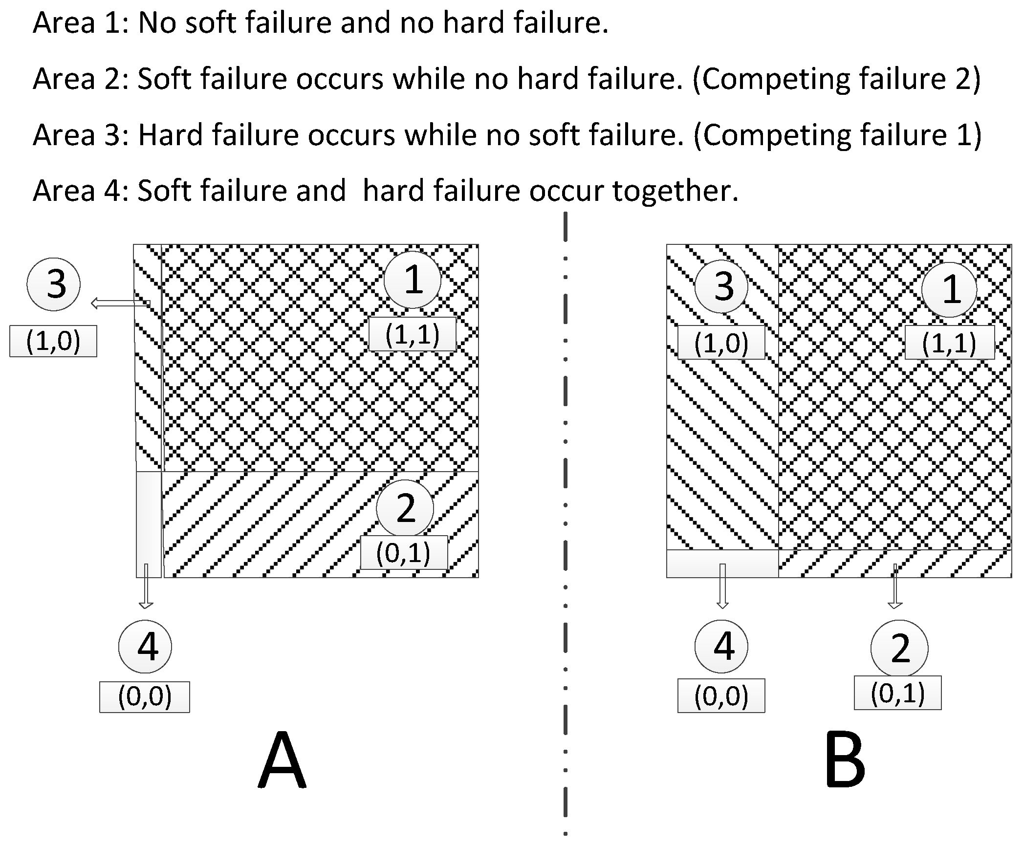
$P_{C{F}_1}\left(x,t\right), P_{C{F}_2}\left(x,t\right)$	Competing failure probability (abbreviated by CFP)
$M{R}_{system}\left(x,t\right)$	Modified system reliability probability (abbreviated by MSRP)
$M{P}_{C{F}_1}\left(x,t\right), M{P}_{C{F}_2}\left(x,t\right)$	Modified competing failure probability (abbreviated by MCFP)

3. Modeling for Risk Modes

3.1. Modeling for Soft Failure

Generally, the overall degradation $X_s\left(t\right)$ consists of two parts, the pure degradation X(t) caused by wastage such as wear, corrosion, and aging and the instantaneous degradation increments S(t) caused by random shocks. As soon as the total degradation exceeds its threshold, soft failure occurs. A linear degradation path X(t) = φ + βt is used to model pure degradation, where the initial degradation value φ and rate β can be constants or random variables. Random shocks arrive with a Poisson process {N(t), t ≥ 0}, whose rate is λ. The size of each shock is a random variable W_i. Each shock may cause an instantaneous increment following the same distribution, no matter how large the shock size is in previous studies.

Actually, the increment caused by a shock cannot be the same or the same distribution if the shock sizes are different. It is easy to understand that a larger shock size is more likely to cause a larger instantaneous increment. For example, wear on a hinge leads to degeneration over time, and shock will also cause degradation incrementally. Shock 1 has a very small size, just like being lightly tickled by a finger. Shock 2 has a larger size, like being struck by a hammer. Shock 3 has the maximal size among these three shocks, like a heavy strike by a motor vehicle. Supposing no hard failure occurs, the damages caused by these three shocks cannot be the same, obviously. Shocks like shock 1 may cause nothing to the systems, so there will be no degradation increment. Shocks like shock 2 and shock 3 will lead to degradation increments, while the increments caused by shock 3 are even bigger than those by shock 2. Therefore, the shocks could be classified into various types according to their shock sizes. At the same time, the degradation increments caused by shocks from different shock types also occur under different distributions.

The new model in the article classifies the shocks into three categories according to their shock sizes. The degradation increments vary with different categories. The shock size of W_is follows a specific distribution. If one shock’s size is under a determined value D₂, it will not cause a degradation increment like W₁, W₂, W₄ in Figure 1. This kind of shock is defined as shock type 1. Shock sizes between D₂ and D₁, like W₃, W₅ in Figure 1, are defined as shock type 2 with instantaneous increment B_j. B_j is i.i.d. random variable with its specific distribution parameters. Similarly, shocks with size between D₁ and hard failure thresholds will lead to another degradation increment C_k with different distribution parameters like W₆ in Figure 1. Additionally, shocks like W₆ are defined as shock type 3.

Shocks arrive with a Poisson process {N(t), t ≥ 0} whose rate is λ. For shock type i, it also follows the Poisson process {N_i(t), t ≥ 0}(i = 1, 2, 3) with rate λ_i. According to stochastic processes theory, the expressions are as follows:

$$\begin{array}{l}N(t)=N_1(t)+N_2(t)+N_3(t)\\ {\lambda }_1=r_1\lambda ,\hspace{1em}{\lambda }_2=r_2\lambda ,\hspace{1em}{\lambda }_3=r_3\lambda \end{array}$$

(1)

where r_i is the ratio of type i shock. Additionally, r_i can be obtained by following expressions.

$$\begin{array}{l}{r}_1=P\left(W_i<D_2\right)\\ r_2=P\left(D_2<W_i<D_1\right)\\ r_3=P\left(D_1<W_i<D_0\right)\end{array}$$

(2)

The cumulative instantaneous increments for degradation change into:

$$S\left(t\right)=\left\{\begin{array}{ll}{\displaystyle \sum _{i=1}^{N_1(t)}{A}_i}+{\displaystyle \sum _{j=1}^{N_2(t)}{B}_j}+{\displaystyle \sum _{k=1}^{N_3(t)}{C}_k},\hspace{1em}& N_i(t)>0,\\ 0,& N_i(t)=0,\end{array}\right.$$

(3)

where A_i is equal to zero when no degradation occurs. B_j and C_k are i.i.d. (Independent Identically Distribution) random variables with different distribution parameters. The cumulative distribution function (CDF) of degradation measurement X_s(t) can be deduced as:

$$\begin{array}{cc}\hfill F_X(x,t)& =P\left(X_S\left(t\right)<x\right)\hfill \\ \hfill & =\sum _{n_3=0}^{n-n_2}\sum _{n_2=0}^n\sum _{n=0}^{\infty }P\left(X\left(t\right)+S\left(t\right)<x|\left(N\right(t)=n,N_2\left(t\right)=n_2,N_3\left(t\right)=n_3)\right)\hfill \\ \hfill & \times P\left(N\left(t\right)=n\right)P\left(N_2\left(t\right)=n_2\right)P\left(N_3\left(t\right)=n_3\right)\hfill \\ \hfill & =\sum _{n_3=0}^{n-n_2}\sum _{n_2=0}^n\sum _{n=0}^{\infty }P\left(X\left(t\right)+\sum _{j=1}^{n_2}{B}_j+\sum _{k=1}^{n_3}{C}_k<x|\left(N\right(t)=n,N_2\left(t\right)=n_2,N_3\left(t\right)=n_3)\right)\hfill \\ \hfill & \times P\left(N\left(t\right)=n\right)P\left(N_2\left(t\right)=n_2\right)P\left(N_3\left(t\right)=n_3\right)\hfill \\ \hfill & =\sum _{n_3=0}^{n-n_2}\sum _{n_2=0}^n\sum _{n=0}^{\infty }\left({\int }_0^x{\int }_0^{u}G(x-u,t){f_B}^{<m>}(u-u_1){f_C}^{<n>}\left(u_1\right)d{u}_{1}du\right)\hfill \\ \hfill & \times \frac{exp(-\lambda t){\left(\lambda t\right)}^n}{n!}\frac{exp(-{\lambda }_{2}t){\left({\lambda }_{2}t\right)}^{n_2}}{n_2!}\frac{exp(-{\lambda }_{3}t){\left({\lambda }_{3}t\right)}^{n_3}}{n_3!}\hfill \end{array}$$

(4)

where G(x,t) denotes the CDF of x(t), and f_B^<m>(u), f_C^<m>(u) means the PDF of the sum of m i.i.d. B_j and n C_k. Moreover, when the instantaneous increments are normally distributed i.i.d., B_j ~ N(μ_B, σ_B²), C_k ~ N(μ_C, σ_C²), and the degradation path is linear with a constant parameter φ and a normal-distributed β ~ N(μ_β, σ_β²), the expression will be more specific:

$$\begin{array}{c}{F}_X(x,t)={\displaystyle \sum _{n_3=0}^{n-n_2}{\displaystyle \sum _{n_2=0}^n{\displaystyle \sum _{n=0}^{\infty }\mathrm{\Phi }\left(\frac{x-({\mu }_{\beta }t+\phi +n_2{\mu }_B+n_3{\mu }_C)}{\sqrt{{\sigma }_{\beta }{}^2{t}^2+n_2{\sigma }_B{}^2+n_3{\sigma }_C{}^2}}\right)}}}\\ \times \frac{\exp (-\lambda t){(\lambda t)}^n}{n!}\frac{\exp (-{\lambda }_{2}t){({\lambda }_{2}t)}^{n_2}}{n_2!}\frac{\exp (-{\lambda }_{3}t){({\lambda }_{3}t)}^{n_3}}{n_3!}\end{array}$$

(5)

where the Φ( ) is the CDF of a standard normal random variable.

3.2. Modeling for Hard Failure

The extreme shock model is used in this paper to model hard failure, which means as soon as the shock size exceeds the thresholds, hard failure occurs. The probability that no hard failure occurs at the ith random shock is

$$P(W_i<D_0)=F_W(D_0)\hspace{1em}i=1,2,3,\cdots$$

(6)

where F_W denotes the CDF of W_i. The expression becomes Equation (7) when W_i follows a normal distribution.

$$F_W(D_0)=\mathrm{\Phi }\left(\frac{D_0-{\mu }_W}{{\sigma }_W}\right)$$

(7)

Accordingly, the system survives after the shock at time t is

$$R_H={\displaystyle \sum _{n=1}^{\infty }P\left({\displaystyle \underset{i=1}{\overset{n}{\cap }}\left\{W_i<D_0\right\}}|(N(t)=n)\right)P(N(t)=n)}={\displaystyle \sum _{n=1}^{\infty }{F}_W{}^n\left(D_0\right)}$$

(8)

4. Reliability Assemble

4.1. System Reliability and Competing Failure Analysis

Systems stay reliable when neither the soft failure nor the hard failure occurs. In practice, it is a focus on how the system reliability probability changes with time. Furthermore, soft failure and hard failure compete with each other, so it is also attractive to study the competing failure probability. The competing failure probability means the failure probability for a certain failure mode (soft failure or hard failure) when the other failure mode is normal at time t. If the competing failure probability of one failure mode is much larger than the other, it means that this kind of failure is more likely to occur. Engineers should pay more attention to the failure mode with a larger competing failure probability.

The system survives when no failure occurs. The reliability is the probability that total degradation is smaller than threshold H and each shock size is under D₀.

$$\begin{array}{cc}\hfill R_{System}(H,t)& =\sum _{n_3=0}^{n-n_2}\sum _{n_2=0}^n\sum _{n=0}^{\infty }P\left(\underset{i=1}{\stackrel{n_3}{\cap }}\left\{W_i<D_0\right\},X_s\left(t\right)<H|\left(N\right(t)=n,N_2\left(t\right)=n_2,N_3\left(t\right)=n_3)\right)\hfill \\ \hfill & \times P\left(N\left(t\right)=n,N_2\left(t\right)=n_2,N_3\left(t\right)=n_3\right)\hfill \\ \hfill & =\sum _{n_3=0}^{n-n_2}\sum _{n_2=0}^n\sum _{n=0}^{\infty }P\left(\begin{array}{c}\underset{i=1}{\stackrel{n_3}{\cap }}\left\{W_i<D_0\right\},X\left(t\right)+\sum _{j=1}^{n_2}{B}_j+\sum _{k=1}^{n_3}{C}_k<H\left|\left(N\right(t\right)=n,\hfill \\ N_2\left(t\right)=n_2,N_3\left(t\right)=n_3)\hfill \end{array}\right)\hfill \\ \hfill & \times P\left(N\left(t\right)=n\right)P\left(N_2\left(t\right)=n_2\right)P\left(N_3\left(t\right)=n_3\right)\hfill \\ \hfill & =\sum _{n_3=0}^{n-n_2}\sum _{n_2=0}^n\sum _{n=0}^{\infty }{F}_W{\left(D_0\right)}^n\left({\int }_0^H{\int }_0^{u}G(x-u,t){f_B}^{<m>}(u-u_1){f_C}^{<n>}\left(u_1\right)d{u}_{1}du\right)\hfill \\ \hfill & \times \frac{exp(-\lambda t){\left(\lambda t\right)}^n}{n!}\frac{exp(-{\lambda }_{2}t){\left({\lambda }_{2}t\right)}^{n_2}}{n_2!}\frac{exp(-{\lambda }_{3}t){\left({\lambda }_{3}t\right)}^{n_3}}{n_3!}\hfill \end{array}$$

(9)

Because shocks are classified into three types, while just the third type may overtake the threshold D₀, the hard failure in Equation (9) should use N₃(t) and n₃ instead of N(t) in Equation (8).

If W_i, B_j, and C_k follow a normal distribution, the reliability will be expressed as Equation (10).

$$\begin{array}{ll}{R}_{System}(H,t)& ={\displaystyle \sum _{n_3=0}^{n-n_2}{\displaystyle \sum _{n_2=0}^n{\displaystyle \sum _{n=0}^{\infty }{F}_W{\left(D_0\right)}^{n_3}\mathrm{\Phi }\left(\frac{H-({\mu }_{\beta }t+\phi +n_2{\mu }_B+n_3{\mu }_C)}{\sqrt{{\sigma }_{\beta }{}^2{t}^2+n_2{\sigma }_B{}^2+n_3{\sigma }_C{}^2}}\right)}}}\\ & \times \frac{\exp (-\lambda t){(\lambda t)}^n}{n!}\frac{\exp (-{\lambda }_{2}t){({\lambda }_{2}t)}^{n_2}}{n_2!}\frac{\exp (-{\lambda }_{3}t){({\lambda }_{3}t)}^{n_3}}{n_3!}\end{array}$$

(10)

There are two scenarios for competing failure probability. The first is the probability that hard failure occurs when no soft failure occurs, while the other is the probability that soft failure occurs when no hard failure occurs. Specifically, we call them competing failure 1 and competing failure 2.

For competing failure 1, it requires that hard failure occurs and no soft failure occurs. As we all know, the system stops when failure occurs. Supposing there are n₃ times type-3 shocks, the shock failure must occur at the n3rd shock. The reliability expression is

$$\begin{array}{cc}\hfill P_{C{F}_1}(H,t)& =\sum _{n_3=1}^{n-n_2}\sum _{n_2=0}^n\sum _{n=1}^{\infty }P\left(\begin{array}{c}\underset{i=1}{\stackrel{n_3-1}{\cap }}\left\{W_i<D_0\right\},W_{n_3}>D_0,X_s\left(t\right)<H\left|\left(N\right(t\right)=n,\hfill \\ N_2\left(t\right)=n_2,N_3\left(t\right)=n_3)\hfill \end{array}\right)\hfill \\ & \times P\left(N\left(t\right)=n,N_2\left(t\right)=n_2,N_3\left(t\right)=n_3\right)\hfill \\ & =\sum _{n_3=1}^{n-n_2}\sum _{n_2=0}^n\sum _{n=1}^{\infty }P\left(\begin{array}{c}\underset{i=1}{\stackrel{n_3-1}{\cap }}\left\{W_i<D_0\right\},W_{n_3}>D_0,X\left(t\right)+\sum _{j=1}^{n_2}{B}_j+\sum _{k=1}^{n_3}{C}_k<H\left|\left(N\right(t\right)=n,\hfill \\ N_2\left(t\right)=n_2,N_3\left(t\right)=n_3)\hfill \end{array}\right)\hfill \\ & \times P\left(N\left(t\right)=n\right)P\left(N_2\left(t\right)=n_2\right)P\left(N_3\left(t\right)=n_3\right)\hfill \\ & =\sum _{n_3=1}^{n-n_2}\sum _{n_2=0}^n\sum _{n=1}^{\infty }{F}_W{\left(D_0\right)}^{n_3-1}\left(1-F_W\left(D_0\right)\right)\left({\int }_0^H{\int }_0^{u}G(x-u,t){f_B}^{<m>}(u-u_1){f_C}^{<n>}\left(u_1\right)d{u}_{1}du\right)\hfill \\ & \times \frac{exp(-\lambda t){\left(\lambda t\right)}^n}{n!}\frac{exp(-{\lambda }_{2}t){\left({\lambda }_{2}t\right)}^{n_2}}{n_2!}\frac{exp(-{\lambda }_{3}t){\left({\lambda }_{3}t\right)}^{n_3}}{n_3!}\hfill \end{array}$$

(11)

For the normal variable, the expression will be

$$\begin{array}{ll}{P}_{C{F}_1}(H,t)& ={\displaystyle \sum _{n_3=0}^{n-n_2}{\displaystyle \sum _{n_2=0}^n{\displaystyle \sum _{n=0}^{\infty }{F}_W{\left(D_0\right)}^{n_3-1}\left(1-F_W\left(D_0\right)\right)\mathrm{\Phi }\left(\frac{H-({\mu }_{\beta }t+\phi +n_2{\mu }_B+n_3{\mu }_C)}{\sqrt{{\sigma }_{\beta }{}^2{t}^2+n_2{\sigma }_B{}^2+n_3{\sigma }_C{}^2}}\right)}}}\\ & \times \frac{\exp (-\lambda t){(\lambda t)}^n}{n!}\frac{\exp (-{\lambda }_{2}t){({\lambda }_{2}t)}^{n_2}}{n_2!}\frac{\exp (-{\lambda }_{3}t){({\lambda }_{3}t)}^{n_3}}{n_3!}\end{array}$$

(12)

Competing failure 2 means soft failure occurs while no hard failure occurs. The probability could be expressed by

$$\begin{array}{cc}\hfill P_{C{F}_2}(H,t)& =\sum _{n_3=0}^{n-n_2}\sum _{n_2=0}^n\sum _{n=0}^{\infty }P\left(\underset{i=1}{\stackrel{n_3}{\cap }}\left\{W_i<D_0\right\},X_s\left(t\right)>H|\left(N\right(t)=n,N_2\left(t\right)=n_2,N_3\left(t\right)=n_3)\right)\hfill \\ & \times P\left(N\left(t\right)=n,N_2\left(t\right)=n_2,N_3\left(t\right)=n_3\right)\hfill \\ & =\sum _{n_3=0}^{n-n_2}\sum _{n_2=0}^n\sum _{n=0}^{\infty }P\left(\begin{array}{c}\underset{i=1}{\stackrel{n_3}{\cap }}\left\{W_i<D_0\right\},X\left(t\right)+\sum _{j=1}^{n_2}{B}_j+\sum _{k=1}^{n_3}{C}_k>H\left|\left(N\right(t\right)=n,\hfill \\ N_2\left(t\right)=n_2,N_3\left(t\right)=n_3)\hfill \end{array}\right)\hfill \\ & \times P\left(N\left(t\right)=n\right)P\left(N_2\left(t\right)=n_2\right)P\left(N_3\left(t\right)=n_3\right)\hfill \\ & =\sum _{n_3=0}^{n-n_2}\sum _{n_2=0}^n\sum _{n=0}^{\infty }{F}_W{\left(D_0\right)}^n\left[1-\left({\int }_0^H{\int }_0^{u}G(x-u,t){f_B}^{<m>}(u-u_1){f_C}^{<n>}\left(u_1\right)d{u}_{1}du\right)\right]\hfill \\ & \times \frac{exp(-\lambda t){\left(\lambda t\right)}^n}{n!}\frac{exp(-{\lambda }_{2}t){\left({\lambda }_{2}t\right)}^{n_2}}{n_2!}\frac{exp(-{\lambda }_{3}t){\left({\lambda }_{3}t\right)}^{n_3}}{n_3!}\hfill \end{array}$$

(13)

$$\begin{array}{ll}{P}_{C{F}_2}(H,t)=& {\displaystyle \sum _{n_3=0}^{n-n_2}{\displaystyle \sum _{n_2=0}^n{\displaystyle \sum _{n=0}^{\infty }{F}_W{\left(D_0\right)}^{n_3}\left[1-\mathrm{\Phi }\left(\frac{H-({\mu }_{\beta }t+\phi +n_2{\mu }_B+n_3{\mu }_C)}{\sqrt{{\sigma }_{\beta }{}^2{t}^2+n_2{\sigma }_B{}^2+n_3{\sigma }_C{}^2}}\right)\right]}}}\\ & \times \frac{\exp (-\lambda t){(\lambda t)}^n}{n!}\frac{\exp (-{\lambda }_{2}t){({\lambda }_{2}t)}^{n_2}}{n_2!}\frac{\exp (-{\lambda }_{3}t){({\lambda }_{3}t)}^{n_3}}{n_3!}\end{array}$$

(14)

Competing failure probabilities are another effective way to demonstrate the system status besides the system reliability. Even for the same system reliability value, the competing failure probabilities for the same risk mode may be different. Figure 2 introduces the problem. There are four possible combinations for soft risk mode and hard risk mode. The proportion of area 1 to the total area denotes system reliability. The system reliabilities in Figure 2A,B are the same, while the proportions of area 2 (competing failure 2) are different. It is the same as area 3. In addition, the soft failure needs to pay more attention in Figure 2A, while it becomes hard failure in Figure 2B even though the system reliabilities are the same. Thus, the competing failure probabilities are also necessary.

4.2. Deriving of the Modified Probability

For systems under soft risk and hard risk, either the soft failure or the hard failure occurs when the system fails. It is impractical for both failures to occur together, just like Figure 2 shows. The reliability calculated by Equations (9) and (10) denotes the rate of area 1, specifically, $\frac{\mathrm{Area}1}{\mathrm{Area}1+\mathrm{Area}2+\mathrm{Area}3+\mathrm{Area}4}$. Similarly, the competing failure probability calculated by Equations (11)–(14) denotes the rate of area 2 and area 3, $\frac{\mathrm{Area}2}{\mathrm{Area}1+\mathrm{Area}2+\mathrm{Area}3+\mathrm{Area}4}$ and $\frac{\mathrm{Area}3}{\mathrm{Area}1+\mathrm{Area}2+\mathrm{Area}3+\mathrm{Area}4}$. In fact, it is not perfect because area 4 is an impossible event for a system under competing risk modes. The exact probabilities should be $\frac{\mathrm{Area}1}{\mathrm{Area}1+\mathrm{Area}2+\mathrm{Area}3}$,$\frac{\mathrm{Area}2}{\mathrm{Area}1+\mathrm{Area}2+\mathrm{Area}3}$, and $\frac{\mathrm{Area}3}{\mathrm{Area}1+\mathrm{Area}2+\mathrm{Area}3}$ which are more reasonable and logical.

The modified system reliability and competing failure probabilities would be expressed by the following functions of Equations (15)–(17).

$$M{R}_{System}(x,t)=\frac{R_{System}(x,t)}{R_{System}(x,t)+P_{C{F}_1}(x,t)+P_{C{F}_2}(x,t)}$$

(15)

$$M{P}_{C{F}_1}(x,t)=\frac{P_{C{F}_1}(x,t)}{R_{System}(x,t)+P_{C{F}_1}(x,t)+P_{C{F}_2}(x,t)}$$

(16)

$$M{P}_{C{F}_2}(x,t)=\frac{P_{C{F}_2}(x,t)}{R_{System}(x,t)+P_{C{F}_1}(x,t)+P_{C{F}_2}(x,t)}$$

(17)

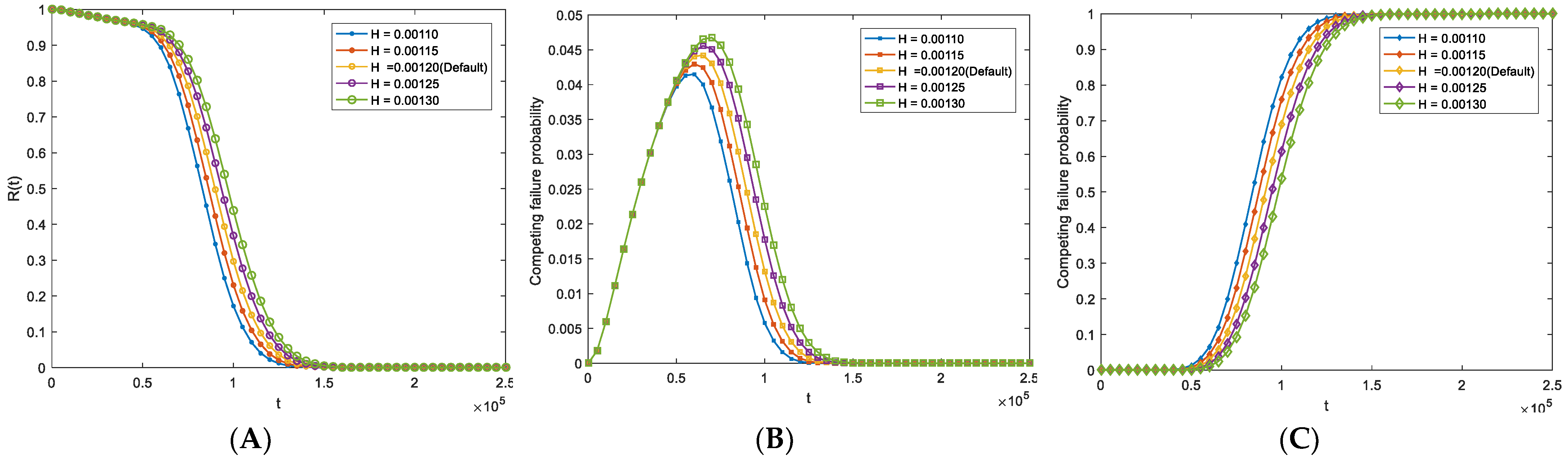
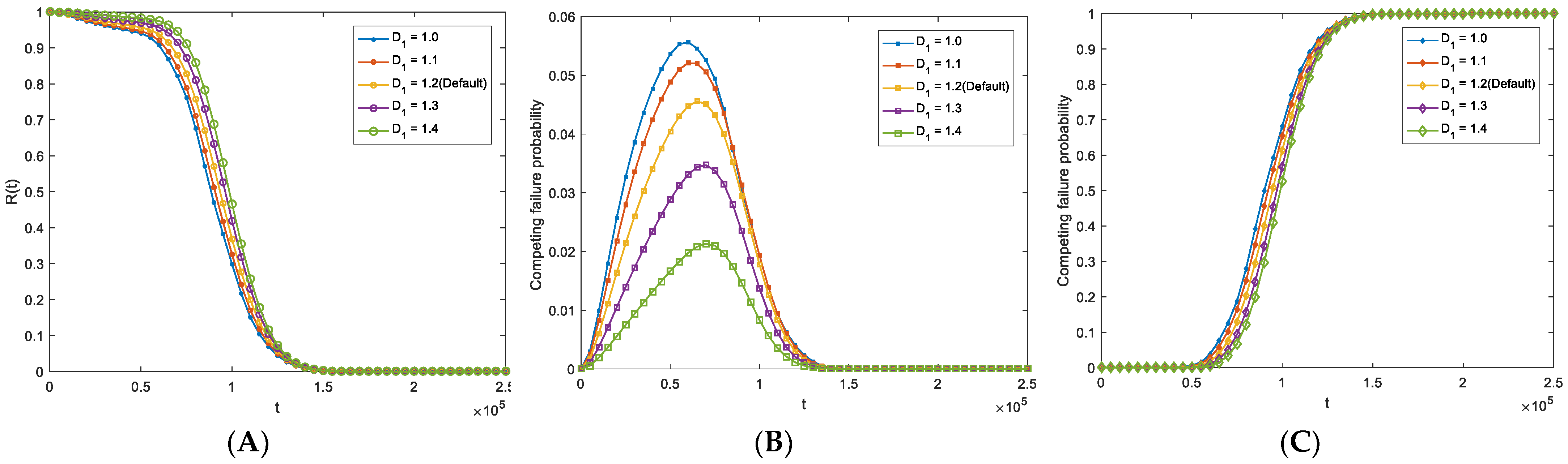
5. Numerical Case: An MEMS Application

The numerical case is a micro-engine consisting of orthogonal linear comb drive actuators mechanically connected to a rotating gear whose data comes from the related literature [4]. MEMS is widely used in industry, specifically in vibration monitoring [25] and micropumps [26]. Due to the working condition and environment, some industry systems with MEMS are always under external shocks and wear processes. Thus, the micro-engine experiences two competing failure processes: soft failure and hard failure. Soft failure is the wear between the gear and the pin joint. The wear volume is caused by the aging degradation process and instantaneous increments due to shock loads [4]. Additionally, different shock loads will lead to different increments. When the total wear volume exceeds the threshold H, the system will fail because of soft failure. Furthermore, the shock loads may cause the fracture of springs, which is regarded as a hard failure. The models presented in this paper are used to study the reliability of the micro-engine. This widely used example is acknowledged to demonstrate the validity of methods or models.

The necessary parameters for calculation are listed in

Table 1. Parameter Values.

Parameters	Values	Sources
H	0.00125	Tanner [27]
D0	1.5	Tanner [27]
D1	1.2	Assumption
D2	1.0	Assumption
φ	0	Tanner [27]
β	~N (μβ, σβ2) μβ = 8.4823 × 10−9 μm3 σβ = 6.0016 × 10−10 μm3	Tanner [2]
Wi	~N (μW, σW2) μW = 1.2 Gpa σW = 0.2 Gpa	Jiang L. [4]
λ	5 × 10 − 5/revolution	Jiang L. [4]
Bi	~N (μB, σB2) μB = 1.2 × 10−4 μm3 σB = 2 × 10−10 μm3	Assumption
Ci	~N (μC, σC2) μC = 1.8×10−4 μm3 σC = 2×10−10 μm3	Assumption

. Wear degradation (soft failure) threshold H, maximum fracture strength D₀, and degradation path parameters φ and β are obtained from Sandia’s experimental results and other references. W_i and λ are normally distributed random variables according to references [27]. The degradation instantaneously increases variables B_i and C_i, which are supposed to be normal distributions.

The ratios calculated by Equation (2) are 0.1586, 0.3413, and 0.4331. General reliability and competing failure probabilities are calculated by Equations (10), (12) and (14), and modified values of system reliability and competing failure probabilities are calculated by Equations (15)–(17), which are illustrated in Figure 3. Figure 3A shows that the modified system reliability value is greater than the general reliability. The reason is that modified reliability eliminates the situation in which both failures occur together, which is impossible. Figure 3B,C show the competing failure and modified competing failure for soft and hard failure. Modified competing failure in Figure 3C indicates that the system certainly fails because of degradation when working circulation is large enough, which is more logical than general competing failure. Thus, the probabilities following are all modified values.

To explore the sensitivity of parameters on reliability and competing failure probability, the results by different parameter values are illustrated. In Figure 4, the system reliability and probability of hard failure while there is no soft failure increases with H at a fixed time. It is easy to understand that the larger the hard threshold H, the less possible for hard failure and system failure. Meanwhile, Figure 4C demonstrates that the competing failure probability 2 decreases with H because of the same reason. After t reaches about 1.5 × 10⁵, the system reliability decreases to 0, as Figure 4A shows. The wastage of the system is so serious after sufficient working circulation that the system will fail because of soft failure definitely. Figure 4B,C demonstrates the inference, too.

In Figure 5, the probabilities with different rates λ are calculated. It can be observed that larger λ will lead to lower system reliability and higher competing failure probability 2. The reason is that larger λ means more frequent shocks, including those that can destroy the system. However, the MCFP 1 increases with λ at the initial working time, while it decreases with λ at the later working period after a critical point.

Figure 6 and Figure 7 show the impacts on MSRP and MCFP of different D₁ and D₂. The impacts on MSRP and MCFP 2 are the same for D₁ and D₂. The increase of D₁ or D₂ will increase MSRP and decrease MCFP 2. By comparison, MCFP 1 decreases with D₁ increasing, while it increases with D₂ increasing. Particularly, the MCFP 1 in Figure 6B is so sensitive to D₁ that the maximum value when D₁ equals 1.0 is almost four times larger than it is at 1.4.

In conclusion, the reliability performance will be different with different parameter values. The threshold H, D₁, and D₂ are properties of the product itself. Higher and more credible threshold values will lead to better system reliability performance, according to our results. The rate λ of the Poisson process indicated the frequency of external shocks. Larger λ means more frequent shocks, which will decrease the system reliability performance. An adaptive working environment with a small enough λ will benefit the reliability.

6. Conclusions and Summary

We develop a reliability model for systems under competing risk modes of soft failure and hard failure. The presented model classifies the random shocks into three types according to their sizes. Besides system reliability, competing failure probabilities are also studied. To make the results more accurate and logical, the modified values of system reliability and competing failure probabilities are obtained.

The hard failures are modeled by the general extreme shock model, while the soft failure is composed of pure degradation and instantaneous degradation caused by extreme shock. The degradation increments caused by random shocks are classified into three types according to their size in this paper, which is more logical. Besides the system reliability, competing failure probability for specific risk modes is derived in this paper. Competing failure probability indicates the failure probability for a certain failure mode (soft failure or hard failure) when the other failure mode is normal. Competing failure probability is significant to find out which risk mode is more likely to occur during the working process. For a system under competing risk modes, it is impossible for both risk modes to occur together. The accurate probabilities need to elide this situation instead of calculating by distribution expression directly. The accurate probabilities include the modified system reliabilities and modified competing failure probabilities for both risk modes. The numerical case indicates the presented model is more reasonable in dealing with the practice problems. Sensitivities of typical parameters with changing values are analyzed.

For further research, the maintenance based on the presented model can be studied. The exact values of thresholds (like D₀, D₁, and D₂) need to be set according to a practice experiment or engineering case.

References

1. Li, W.; Pham, H. Reliability modeling of multi-state degraded systems with multi-competing failures and random shocks. IEEE Trans. Reliab. 2005, 54, 297–303. [Google Scholar] [CrossRef]
2. Peng, H.; Feng, Q.; Coit, D. Reliability and maintenance modeling for systems subject to multiple dependent competing failure processes. IIE Trans. 2011, 43, 12–22. [Google Scholar] [CrossRef]
3. Rafiee, K.; Feng, Q.; Coit, D. Reliability modeling for dependent competing failure processed with changing degradation rate. IIE Trans. 2013, 46, 483–496. [Google Scholar] [CrossRef]
4. Jiang, L.; Feng, Q.; Coit, D. Reliability and Maintenance Modeling for Dependent Competing Failure Processes with Shifting Failure Thresholds. IEEE Trans. Reliab. 2012, 61, 932–948. [Google Scholar] [CrossRef]
5. Pham, H. Safety and Risk Modeling and Its Applications; Springer: London, UK, 2011; pp. 197–218. [Google Scholar]
6. Jiang, L.; Feng, Q.; Coit, D. Reliability assessment of competing risks with generalized mixed shock models. Reliab. Eng. Syst. Saf. 2017, 159, 1–11. [Google Scholar]
7. Nicolai, R.; Dekker, R.; Noortwijk, J. A comparison of models for measurable deterioration: An application to coatings on steel structures. Reliab. Eng. Syst. Saf. 2007, 92, 1635–1650. [Google Scholar] [CrossRef]
8. Si, X.; Zhou, D. A generalized result for degradation model-based reliability estimation. IEEE Trans. Reliab. 2014, 11, 632–637. [Google Scholar] [CrossRef]
9. Xu, D.; Wei, Q.; Chen, Y. Reliability prediction using physics-statistics-based degradation model. IEEE Trans. Compon. 2015, 5, 1573–1581. [Google Scholar]
10. Ma, J.; Yuan, D. Accelerated storage life evaluation of FOG based on drift Brownian movement. J. Chin. Inert. Technol. 2010, 8, 756–760. [Google Scholar]
11. Ren, S.; Zuo, H.; Bai, F. Real-time performance reliability prediction for civil aviation engines based on Brownian motion with drift. J. Aerosp. Power 2009, 24, 2796–2801. [Google Scholar]
12. Cai, J.; Ren, S. Research on Reliability Prediction for Roller-slide Based on Brownian Motion with Drift. China Mech. Eng. 2012, 23, 1408–1412. [Google Scholar]
13. Bai, Z.; Zhao, Y.; Chen, J. Dynamics analysis of planar mechanical system considering revolute clearance joint wear. Tribol. Int. 2013, 64, 85–95. [Google Scholar] [CrossRef]
14. Haneef, M.D.; Randall, R.B.; Smith, W.A.; Peng, Z. Vibration and wear prediction analysis of IC engine bearings by numerical simulation. Wear 2017, 384, 15–27. [Google Scholar] [CrossRef]
15. Jones, N. Slamming damage. J. Ship Res. 1973, 17, 80–86. [Google Scholar] [CrossRef]
16. Nandu, V.; Marimuthu, P. Fracture characteristics of asymmetric high contact ratio spur gear based on strain energy release rate. Eng. Fail. Anal. 2022, 134, 106036. [Google Scholar] [CrossRef]
17. Miyakawa, M. Analysis of incomplete data in competing risks model. IEEE Trans. Reliab. 1984, 33, 293–296. [Google Scholar] [CrossRef]
18. Ye, Z.; Tang, L.; Xu, H. A distribution-based system reliability model under extreme shocks and natural degradation. IEEE Trans. Reliab. 2011, 60, 246–256. [Google Scholar] [CrossRef]
19. Wang, X.; Wang, B.; Niu, Y.; He, Z. Reliability Modeling of Products with Self-Recovery Features for Competing Failure Processes in Whole Life Cycle. Appl. Sci. 2023, 13, 4800. [Google Scholar] [CrossRef]
20. Zheng, M.; Lin, R.; Yu, W. Competing risks data analysis under the accelerated failure time model with missing cause of failure. Ann. Inst. Stat. Math. 2016, 68, 855–876. [Google Scholar] [CrossRef]
21. Luo, W.; Zhang, C.; Chen, X. Accelerated reliability demonstration under competing failure modes. Reliab. Eng. Syst. Saf. 2015, 136, 75–84. [Google Scholar] [CrossRef]
22. Song, S.; Coit, D.; Feng, Q. Reliability for systems of degrading components with distinct component shock sets. Reliab. Eng. Syst. Saf. 2014, 132, 115–124. [Google Scholar] [CrossRef]
23. Song, S.; Coit, D.; Feng, Q. Reliability Analysis for Multi-Component Systems Subject to Multiple Dependent Competing Failure Processes. IEEE Trans. Reliab. 2014, 63, 331–345. [Google Scholar] [CrossRef]
24. Rafiee, K.; Feng, Q.; Coit, D. Condition-based maintenance for repairable deteriorating systems subject to a generalized mixed shock model. IEEE Trans. Reliab. 2015, 64, 1164–1174. [Google Scholar] [CrossRef]
25. Rossi, A.; Bocchetta, G.; Botta, F.; Scorza, A. Accuracy Characterization of a MEMS Accelerometer for Vibration Monitoring in a Rotating Framework. Appl. Sci. 2023, 13, 5070. [Google Scholar] [CrossRef]
26. Chappel, E. Dry Test Methods for Micropumps. Appl. Sci. 2022, 12, 12258. [Google Scholar] [CrossRef]
27. Tanner, D.; Dugger, M. Wear mechanisms in a reliability methodology. Proc. Soc. Photo-Ophical Instrum. Eng. 2003, 4980, 22–40. [Google Scholar]
Figure 1. Competing failure process.
Applsci 13 07490 g001
Figure 2. Risk mode status.
Applsci 13 07490 g002
Figure 3. Comparing probability and modified probability. (A): System Reliability Probability; (B): Competing failure probability 1 (probability of hard failure while there is no soft failure); (C): Competing failure probability 2 (probability of soft failure while there is no hard failure).
Applsci 13 07490 g003
Figure 4. Probability with different H. (A): MSRP; (B): MCFP 1 (Probability of hard failure while there is no soft failure); (C): MCFP 2 (Probability of soft failure while there is no hard failure).
Applsci 13 07490 g004
Figure 5. Probability with different λ. (A): MSRP; (B): MCFP 1 (Probability of hard failure while there is no soft failure); (C): MCFP 2 (Probability of soft failure while there is no hard failure).
Applsci 13 07490 g005
Figure 6. Probability with different D1. (A): MSRP; (B): MCFP 1 (Probability of hard failure while there is no soft failure); (C): MCFP 2 (Probability of soft failure while there is no hard failure).
Applsci 13 07490 g006
Figure 7. Probability with different D2. (A): MSRP; (B): MCFP 1 (Probability of hard failure while there is no soft failure); (C): MCFP 2 (Probability of soft failure while there is no hard failure).
Applsci 13 07490 g007