
LSTM Network for the Oxygen Concentration Modeling of a Wastewater Treatment Plant


Abstract
1. Introduction
2. Related Works
3. Materials and Methods
3.1. Plant Description
3.2. Long Short-Term Memory (LSTM) Network
3.3. AutoRegressive Model with eXogenous Input (ARX) Model
3.3.1. Data Conditioning
3.3.2. Model Structure Estimation
3.3.3. Parameter Estimation
3.4. Description of Datasets
3.5. Performance Indexes
- Index of fitting (): normalized index that indicates how much the prediction matches the real data. For a perfect prediction, it is equal to 100%, and it can also be negative. It is expressed as:
- Pearson correlation coefficient (): measures the linear correlation between two variables and has a value between −1 (total negative correlation) and +1 (total positive correlation).
- Root Mean Squared Error (): shows the Euclidean distance of the predictions from the real data using
4. Results
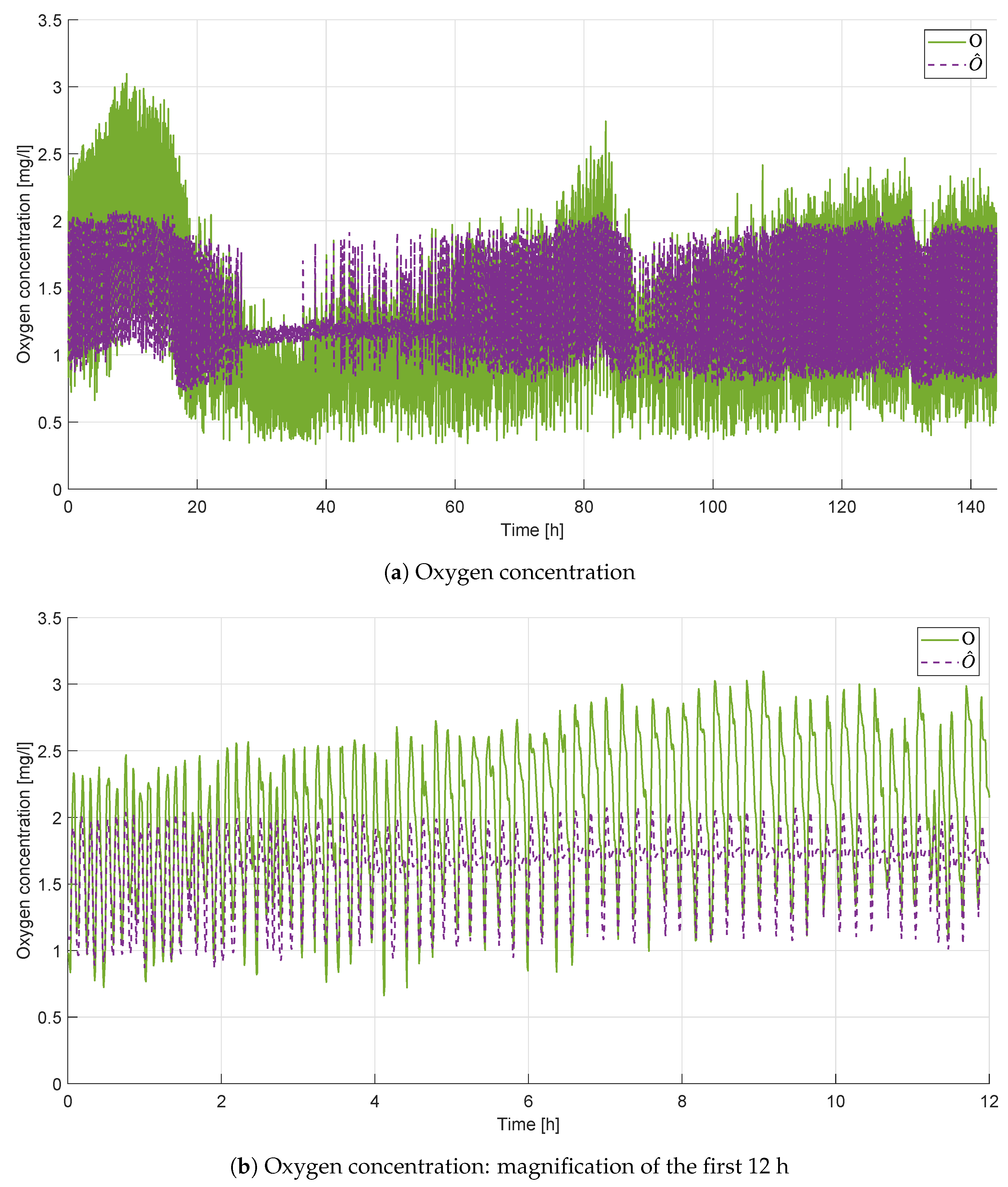
4.1. LSTM Results
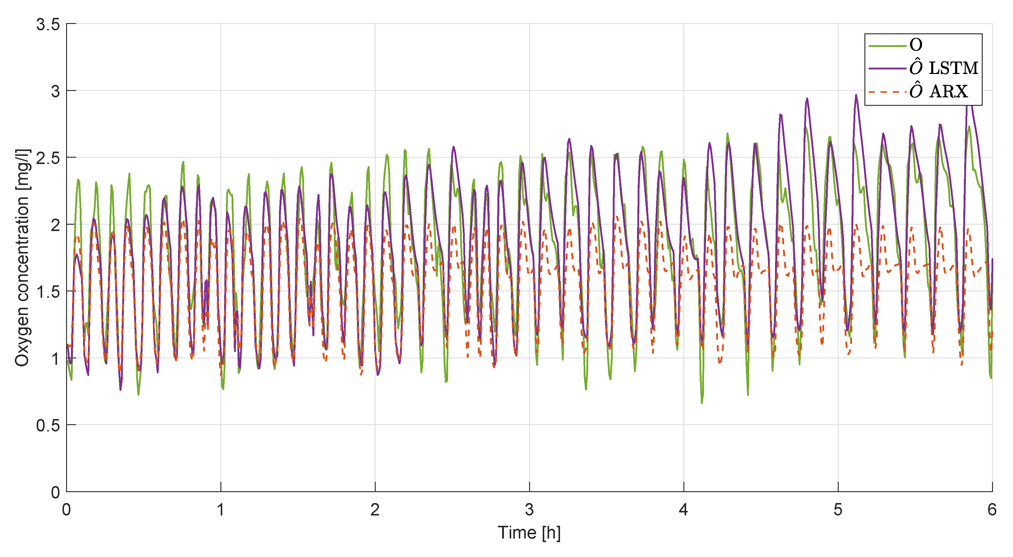
4.2. ARX
4.3. Discussion
5. Conclusions
Supplementary Materials
Author Contributions
Funding
Institutional Review Board Statement
Informed Consent Statement
Data Availability Statement
Conflicts of Interest
Abbreviations
| ASM1 | Activated Sludge Model No. 1 |
| ASM2 | Activated Sludge Model No. 2 |
| ASM3 | Activated Sludge Model No. 3 |
| ARX | Autoregressive exogenous |
| BI-LSTM | BIdirectional-LSTM |
| CAS | Conventional Activated Sludge |
| COD | Chemical Oxygen Demand |
| DEN | Denitrification |
| GRU | Gated Recurrent Unit |
| LSTM | Long Short-Term Memory |
| ML | Machine Learning |
| MSE | Mean Squared Error |
| NN | Neural Network |
| OX-NIT | Oxidation and nitrification |
| RMSE | Root Mean Squared Error |
| RNN | Recurrent Neural Network |
| SCADA | Supervisory Control And Data Acquisition |
| TAMR | Thermophilic Aerobic Membrane Reactor |
| WWTP | WasteWater Treatment Plant |
References
- Hamitlon, R.; Braun, B.; Dare, R.; Koopman, B.; Svoronos, S.A. Control issues and challenges in wastewater treatment plants. IEEE Control Syst. Mag. 2006, 26, 63–69. [Google Scholar]
- Gernaey, K.V.; Van Loosdrecht, M.C.; Henze, M.; Lind, M.; Jørgensen, S.B. Activated sludge wastewater treatment plant modelling and simulation: State of the art. Environ. Model. Softw. 2004, 19, 763–783. [Google Scholar] [CrossRef]
- Henze, M.; Grady, C.L., Jr.; Gujer, W.; Marais, G.; Matsuo, T. A general model for single-sludge wastewater treatment systems. Water Res. 1987, 21, 505–515. [Google Scholar] [CrossRef]
- Gujer, W.; Henze, M.; Mino, T.; Matsuo, T.; Wentzel, M.; Marais, G. The Activated Sludge Model No. 2: Biological phosphorus removal. Water Sci. Technol. 1995, 31, 1–11. [Google Scholar] [CrossRef]
- Gujer, W.; Henze, M.; Mino, T.; Van Loosdrecht, M. Activated sludge model No. 3. Water Sci. Technol. 1999, 39, 183–193. [Google Scholar] [CrossRef]
- Nelson, M.; Sidhu, H.S. Analysis of the activated sludge model (number 1). Appl. Math. Lett. 2009, 22, 629–635. [Google Scholar] [CrossRef]
- Nelson, M.; Sidhu, H.S.; Watt, S.; Hai, F.I. Performance analysis of the activated sludge model (number 1). Food Bioprod. Process. 2019, 116, 41–53. [Google Scholar] [CrossRef]
- Gujer, W. Activated sludge modelling: Past, present and future. Water Sci. Technol. 2006, 53, 111–119. [Google Scholar] [CrossRef]
- Sin, G.; Al, R. Activated sludge models at the crossroad of artificial intelligence—A perspective on advancing process modeling. Npj Clean Water 2021, 4, 1–7. [Google Scholar] [CrossRef]
- Ogunmolu, O.; Gu, X.; Jiang, S.; Gans, N. Nonlinear systems identification using deep dynamic neural networks. arXiv 2016, arXiv:1610.01439. [Google Scholar]
- Siami-Namini, S.; Tavakoli, N.; Namin, A.S. A comparison of ARIMA and LSTM in forecasting time series. In Proceedings of the 2018 17th IEEE International Conference on Machine Learning and Applications (ICMLA), Orlando, FL, USA, 17–20 December 2018; pp. 1394–1401. [Google Scholar]
- Hirose, N.; Tajima, R. Modeling of rolling friction by recurrent neural network using LSTM. In Proceedings of the 2017 IEEE international conference on robotics and automation (ICRA), Singapore, 29 May–3 June 2017; pp. 6471–6478. [Google Scholar]
- Cerna, S.; Guyeux, C.; Arcolezi, H.H.; Couturier, R.; Royer, G. A comparison of LSTM and XGBoost for predicting firemen interventions. In Trends and Innovations in Information Systems and Technologies; Springer: Berlin/Heidelberg, Germany, 2020; Volume 2, pp. 424–434. [Google Scholar]
- Chen, R.; Jin, X.; Laima, S.; Huang, Y.; Li, H. Intelligent modeling of nonlinear dynamical systems by machine learning. Int. J.-Non-Linear Mech. 2022, 142, 103984. [Google Scholar] [CrossRef]
- Song, W.; Gao, C.; Zhao, Y.; Zhao, Y. A time series data filling method based on LSTM—taking the stem moisture as an example. Sensors 2020, 20, 5045. [Google Scholar] [CrossRef] [PubMed]
- Gonzalez, J.; Yu, W. Non-linear system modeling using LSTM neural networks. IFAC-PapersOnLine 2018, 51, 485–489. [Google Scholar] [CrossRef]
- De la Fuente, L.A.; Ehsani, M.R.; Gupta, H.V.; Condon, L.E. Towards Interpretable LSTM-based Modelling of Hydrological Systems. EGUsphere 2023, 2023, 1–29. [Google Scholar]
- Rajendra, P.; Brahmajirao, V. Modeling of dynamical systems through deep learning. Biophys. Rev. 2020, 12, 1311–1320. [Google Scholar] [CrossRef]
- Hreiz, R.; Latifi, M.; Roche, N. Optimal design and operation of activated sludge processes: State-of-the-art. Chem. Eng. J. 2015, 281, 900–920. [Google Scholar] [CrossRef]
- Collivignarelli, M.C.; Abbà, A.; Bertanza, G.; Setti, M.; Barbieri, G.; Frattarola, A. Integrating novel (thermophilic aerobic membrane reactor-TAMR) and conventional (conventional activated sludge-CAS) biological processes for the treatment of high strength aqueous wastes. Bioresour. Technol. 2018, 255, 213–219. [Google Scholar] [CrossRef] [PubMed]
- Collivignarelli, M.; Abbà, A.; Frattarola, A.; Manenti, S.; Todeschini, S.; Bertanza, G.; Pedrazzani, R. Treatment of aqueous wastes by means of Thermophilic Aerobic Membrane Reactor (TAMR) and nanofiltration (NF): Process auditing of a full-scale plant. Environ. Monit. Assess. 2019, 191, 1–17. [Google Scholar] [CrossRef] [PubMed]
- Collivignarelli, M.C.; Abbà, A.; Bertanza, G. Why use a thermophilic aerobic membrane reactor for the treatment of industrial wastewater/liquid waste? Environ. Technol. 2015, 36, 2115–2124. [Google Scholar] [CrossRef]
- Frącz, P. Nonlinear modeling of activated sludge process using the Hammerstein-Wiener structure. In Proceedings of the E3S Web of Conferences; EDP Sciences: Les Ulis, France, 2016; Volume 10, p. 00119. [Google Scholar]
- Hochreiter, S.; Schmidhuber, J. Long short-term memory. Neural Comput. 1997, 9, 1735–1780. [Google Scholar] [CrossRef]
- Gers, F.A.; Schmidhuber, J.; Cummins, F. Learning to forget: Continual prediction with LSTM. Neural Comput. 2000, 12, 2451–2471. [Google Scholar] [CrossRef]
- Llerena Caña, J.P.; García Herrero, J.; Molina López, J.M. Forecasting nonlinear systems with LSTM: Analysis and comparison with EKF. Sensors 2021, 21, 1805. [Google Scholar] [CrossRef]
- Wang, Y. A new concept using LSTM neural networks for dynamic system identification. In Proceedings of the 2017 American control conference (ACC), Seattle, WA, USA, 24–26 May 2017; pp. 5324–5329. [Google Scholar]
- Mohajerin, N.; Waslander, S.L. Multistep prediction of dynamic systems with recurrent neural networks. IEEE Trans. Neural Netw. Learn. Syst. 2019, 30, 3370–3383. [Google Scholar] [CrossRef] [PubMed]
- Gers, F.A.; Schraudolph, N.N.; Schmidhuber, J. Learning precise timing with LSTM recurrent networks. J. Mach. Learn. Res. 2002, 3, 115–143. [Google Scholar]
- Pascanu, R.; Mikolov, T.; Bengio, Y. On the difficulty of training recurrent neural networks. In Proceedings of the International Conference on Machine Learning, PMLR, Singapore, 20–23 February 2013; pp. 1310–1318. [Google Scholar]
- Greff, K.; Srivastava, R.K.; Koutník, J.; Steunebrink, B.R.; Schmidhuber, J. LSTM: A search space odyssey. IEEE Trans. Neural Netw. Learn. Syst. 2016, 28, 2222–2232. [Google Scholar] [CrossRef]
- Pham, V.; Bluche, T.; Kermorvant, C.; Louradour, J. Dropout improves recurrent neural networks for handwriting recognition. In Proceedings of the 2014 14th International Conference on Frontiers in Handwriting Recognition, Hyderabad, India, 4–7 December 2014; pp. 285–290. [Google Scholar]
- Ljung, L. (Ed.) System Identification: Theory for the User, 2nd ed.; Prentice Hall PTR: Upper Saddle River, NJ, USA, 1999. [Google Scholar]
- Söderström, T.; Stoica, P. System Identification; Prentice Hall PTR: Upper Saddle River, NJ, USA, 1989. [Google Scholar]
- Godfrey, K. Correlation methods. Automatica 1980, 16, 527–534. [Google Scholar] [CrossRef]
- O’Malley, T.; Bursztein, E.; Long, J.; Chollet, F.; Jin, H.; Invernizzi, L.; de Marmiesse, G.; Fu, Y.; Podivìn, J.; Schäfer, F.; et al. KerasTuner. 2019. Available online: https://github.com/keras-team/keras-tuner (accessed on 24 March 2021).
- Abadi, M.; Agarwal, A.; Barham, P.; Brevdo, E.; Chen, Z.; Citro, C.; Corrado, G.S.; Davis, A.; Dean, J.; Devin, M.; et al. TensorFlow: Large-Scale Machine Learning on Heterogeneous Systems. In Osdi; USENIX: Savannah, GA, USA, 2016; Volume 16, pp. 265–283. [Google Scholar]
- Chollet, F. Keras. 2015. Available online: https://keras.io (accessed on 12 April 2021).
- System Identification Toolbox Version: 9.16 (R2022a); The MathWorks Inc.: Natick, MA, USA, 2022.
- Taylor, K.E. Summarizing multiple aspects of model performance in a single diagram. J. Geophys. Res. Atmos. 2001, 106, 7183–7192. [Google Scholar] [CrossRef]


| Signal | Component | Range | Selected |
|---|---|---|---|
| order () | 10–17 | 12 | |
| order () | 2–12 | 6 | |
| delay () | 0–5 | 2 | |
| order () | 2–12 | 3 | |
| delay () | 0–10 | 5 | |
| order () | 3–9 | 7 | |
| delay () | 0–10 | 6 |
| Dataset Name | Start Date | End Date |
|---|---|---|
| Dataset 1 | 6 December 2021 | 11 December 2021 |
| Dataset 2 | 15 December 2021 | 20 December 2021 |
| Dataset 3 | 21 December 2021 | 26 December 2021 |
| Dataset 4 | 27 December 2021 | 1 January 2022 |
| Dataset 5 | 1 December 2022 | 6 May 2022 |
| Dataset Name | ||||
|---|---|---|---|---|
| Dataset1 | −0.0054 (0.2724) | −0.4061 (3355) | −0.5910 (25.58) | 0.1471 (2.9851) |
| Dataset2 | −0.3214 (0.1863) | 24.0992 (1608) | −0.7720 (47.79) | −0.3733 (4.5006) |
| Dataset3 | 0.0618 (0.2406) | −14.1781 (3378) | −1.0119 (49.85) | −1.1114 (5.4282) |
| Dataset4 | 0.2023 (0.2633) | −25.0323 (3423) | −1.1772 (46.95) | −1.4870 (4.7857) |
| Dataset5 | 0.1414 (0.3130) | −4.2068 (4826) | 0.8875 (48.54) | 0.8547 (5.9122) |
| Dataset6 | −0.0841 (0.2038) | 19.3180 (3739) | 2.0735 (85.26) | 2.1169 (6.7172) |
| Index | ARX | LSTM |
|---|---|---|
| [%] | 41.20 | 60.56 |
| 0.833 | 0.921 | |
| [mg/L] | 0.307 | 0.206 |
Disclaimer/Publisher’s Note: The statements, opinions and data contained in all publications are solely those of the individual author(s) and contributor(s) and not of MDPI and/or the editor(s). MDPI and/or the editor(s) disclaim responsibility for any injury to people or property resulting from any ideas, methods, instructions or products referred to in the content. |
© 2023 by the authors. Licensee MDPI, Basel, Switzerland. This article is an open access article distributed under the terms and conditions of the Creative Commons Attribution (CC BY) license (https://creativecommons.org/licenses/by/4.0/).
Share and Cite
Toffanin, C.; Di Palma, F.; Iacono, F.; Magni, L. LSTM Network for the Oxygen Concentration Modeling of a Wastewater Treatment Plant. Appl. Sci. 2023, 13, 7461. https://doi.org/10.3390/app13137461
Toffanin C, Di Palma F, Iacono F, Magni L. LSTM Network for the Oxygen Concentration Modeling of a Wastewater Treatment Plant. Applied Sciences. 2023; 13(13):7461. https://doi.org/10.3390/app13137461
Chicago/Turabian StyleToffanin, Chiara, Federico Di Palma, Francesca Iacono, and Lalo Magni. 2023. "LSTM Network for the Oxygen Concentration Modeling of a Wastewater Treatment Plant" Applied Sciences 13, no. 13: 7461. https://doi.org/10.3390/app13137461
APA StyleToffanin, C., Di Palma, F., Iacono, F., & Magni, L. (2023). LSTM Network for the Oxygen Concentration Modeling of a Wastewater Treatment Plant. Applied Sciences, 13(13), 7461. https://doi.org/10.3390/app13137461