Vibration Response Law of Aircraft Taxiing under Random Roughness Excitation

Abstract

Understanding the vibration response patterns of aircraft taxiing under runway roughness excitation is crucial for aircraft design and runway performance evaluation. In this paper, we establish pavement roughness models for both asphalt and concrete surfaces, taking into account their unique structural characteristics. We construct a six-degrees-of-freedom aircraft model using multi-rigid-body system dynamics theory and employ the pseudo-excitation method to examine the influence of pavement roughness types on the steady vibration response of aircraft taxiing at constant speeds. Furthermore, we analyze the non-stationary vibration response patterns of aircraft during takeoff and landing taxiing using the method of instantaneous frequency response function with space frequency. Lastly, we explore the effect of stochastic structural parameters on aircraft vibration response using the Monte Carlo method. Our findings reveal that the roughness power spectrum differs between asphalt and concrete pavements, and the established roughness models in this paper demonstrate a strong fit (R2 > 0.95). The type of pavement roughness has a relatively minor impact on the power spectral density distribution of the aircraft vibration response, suggesting that the same roughness model can be used for both asphalt and concrete pavements when high accuracy is not required. The power spectral density distribution of aircraft vibration response varies across different motion attitudes, with the vibration response during landing being significantly larger than that during takeoff. Among the aircraft structural parameters, the randomness of the sprung mass has the most substantial effect on the aircraft vibration response, potentially causing the variation coefficient of dynamic load on the front landing gear to exceed 0.11. Tire stiffness comes next, which can lead to the variation coefficient of dynamic load on the main landing gear reaching 0.07. The results have a guiding role in optimizing aircraft structure design and ensuring pavement performance.

1. Introduction

The airport runway functions as a crucial support platform for aircraft during taxiing, takeoff, and landing. Owing to a combination of factors such as construction variability, external environment, aircraft loading, and other uncertainties, the pavement exhibits random roughness. Pavement roughness is the vertical deviation of the pavement surface relative to the ideal plane. When subjected to random roughness excitation, high-speed taxiing aircraft experience random vibrations, which can negatively impact passenger comfort, accelerate fatigue damage to aircraft components, cause dynamic damage to runway structures, and even compromise flight safety [1]. As a result, comprehending the vibration response patterns of aircraft under random roughness excitation is vital for optimizing aircraft structural design, ensuring runway structure safety, and maintaining operational safety standards.

Numerous studies have demonstrated that road surface or pavement roughness can be characterized as an ergodic, steady Gaussian stochastic process with zero mean, and its statistical properties can be represented by power spectral density (PSD) [2]. In the field of road research, various roughness models have been developed using PSD through the analysis of measured road roughness data [3,4,5,6,7]. However, runway roughness studies are limited by the available data samples, resulting in few investigations into the power spectrum of runway roughness. For instance, Houbolt proposed a PSD expression for airport pavement roughness based on measuring the relative elevation data of longitudinal sections at only two runways, which lacks representativeness [8]. Most researchers have directly adopted road surface roughness models when studying runway roughness [9,10,11,12]. Nevertheless, this approach can introduce significant deviations in the analysis of runway roughness due to the considerable differences between runways and roads concerning structural forms and service object characteristics [13].

In aircraft vibration response research, the majority of scholars utilize measured or simulated pavement roughness samples for time-domain simulations. For instance, Durán and Júnior calculated aircraft acceleration under measured roughness excitation using ProFAA and evaluated pavement roughness accordingly [14]. Dong et al. simulated the pavement roughness curve with the harmonic superposition method and calculated the taxiing dynamic load of a four-degrees-of-freedom aircraft using the Full method [15]. Cheng et al. and Shi et al. employed the filtered white noise method or harmonic superposition method to generate pavement roughness, and determined the dynamic load coefficient of the six-degrees-of-freedom (6-DOF) model at different speeds using Simulink [16,17]. Liu et al. used the cosine function as the roughness input and analyzed the superposition effect of aircraft vibration with automatic dynamic analysis of mechanical systems (ADAMS) [18]. Qian et al. applied PSD to reconstruct runway roughness and investigated the aircraft taxiing dynamic load using ADAMS [19]. However, measured or simulated single roughness curves only represent pavement roughness excitation at a certain probability level during the runway’s long-term service. Single deterministic time history analysis based on this does not adequately reflect the random vibration characteristics of the aircraft.

To address this limitation, several researchers have conducted frequency domain analyses based on random vibration theory, establishing a direct correlation between the power spectrum input of pavement roughness and the power spectrum output of aircraft vibration response. For instance, Kirk and Perry used the PSD method to analyze the vibration response of a simplified multiple-degrees-of-freedom aircraft under stationary random excitation [20]. Tung solved the single-degree-of-freedom vibration problem of the aircraft using random vibration theory [21]. Nie and Kortum employed the equivalent linearization method to address the nonlinear parameters of the landing gear and examined random vibration during taxiing using the PSD method [22]. Wang applied the pseudo-excitation method (PEM) to compute the dynamic response of unmanned aerial vehicle landing gear under non-stationary random excitation [23]. Liu et al. obtained the vibration response of a two-degrees-of-freedom aircraft–runway coupling system under roughness excitation using the PEM [24]. However, most of these studies employed simplified aircraft models that were unable to capture the characteristics of a large wheelbase and significant spatial vibration of the aircraft.

In this paper, we address the unique structural characteristics of asphalt and concrete pavements by establishing corresponding pavement roughness models using PSD. We derive the motion balance equations of a 6-DOF aircraft under roughness excitation following D’Alembert’s principle. We then use the PEM, the method of instantaneous frequency response function with spatial frequency, and the Monte Carlo method to calculate the PSD distribution of acceleration at the center of gravity (CGA), acceleration at the pilot station (PSA), dynamic load coefficient of the nose landing gear (NGDLC), and dynamic load coefficient of the main landing gear (MGDLC) under various operating conditions. This approach allows us to reveal the vibration response laws of aircraft taxiing under different pavement types, motion attitudes, and stochastic structural parameters. The results can be applied to optimize aircraft design methods and improve the accuracy of pavement roughness evaluation.

2. Random Vibration Models

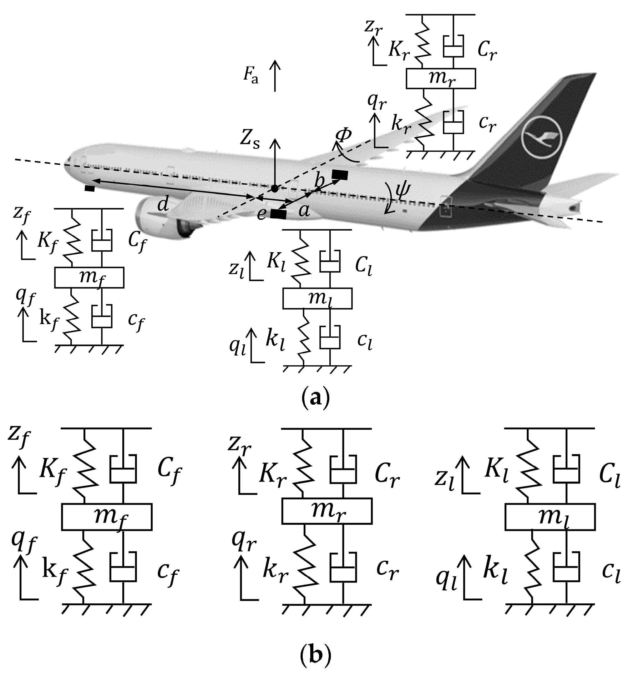
2.1. Aircraft Nonlinear Ground Dynamics Model

Throughout the taxiing process, pavement roughness excitation is transmitted through the tire to the landing gear, which absorbs some of the energy and transfers the vibration to the fuselage. The aircraft is a typical nonlinear model due to the strong nonlinearity of both the tire and the landing gear. In frequency domain dynamic response analysis, nonlinear elements are typically represented by equivalent linear elements. Therefore, in this section, the nonlinear elements are initially represented by equivalent linear letters (with the equivalent linearization process described in the next section), and the nonlinear aircraft model is established.

Initially, based on the theory of multi-rigid-body system dynamics, the aircraft is simplified into two parts: the sprung mass and unsprung mass. Additionally, the mechanical properties of the landing gear buffer and the tire are simulated as a spring-plus-damping model, and the lift, $F_{\mathrm{s}}$, is applied to the center of gravity of the aircraft during takeoff and landing on the runway in a straight line. This yields the ground dynamics model of the 6-DOF aircraft [25], as illustrated in Figure 1.

At any given moment, the aircraft is in a state of dynamic equilibrium. Therefore, the motion balance equations for each degree of freedom of the aircraft ground dynamics model under pavement roughness excitation can be derived using the D’Alembert principle.

The vertical vibration balance equation for the sprung mass is shown as Equation (1).

$$\begin{gathered} M_{\mathrm{s}}{\ddot{Z}}_{\mathrm{s}}+C_{\mathrm{f}}\left({\dot{Z}}_{\mathrm{s}}+d\dot{\Phi }-{\dot{z}}_{\mathrm{f}}\right)+K_{\mathrm{f}}\left(Z_{\mathrm{s}}+d\Phi -z_{\mathrm{f}}\right)+C_{\mathrm{r}}\left({\dot{Z}}_{\mathrm{s}}-e\dot{\Phi }+b\dot{\Psi }-{\dot{z}}_{\mathrm{r}}\right)+K_{\mathrm{r}}(Z_{\mathrm{s}} \\ -e\Phi +b\Psi -z_{\mathrm{r}})+C_{\mathrm{l}}\left({\dot{Z}}_{\mathrm{s}}-e\dot{\Phi }-a\dot{\Psi }-{\dot{z}}_{\mathrm{l}}\right)+K_{\mathrm{l}}\left(Z_{\mathrm{s}}-e\Phi -a\Psi -z_{\mathrm{l}}\right)+F_{\mathrm{a}}=0 \end{gathered}$$

(1)

The pitch rotation balance equation for the sprung mass is shown as Equation (2).

$$\begin{gathered} I_x\ddot{\Phi }+C_{\mathrm{f}}\left({\dot{Z}}_{\mathrm{s}}+d\dot{\Phi }-{\dot{z}}_{\mathrm{f}}\right)d+K_{\mathrm{f}}\left(Z_{\mathrm{s}}+d\Phi -z_{\mathrm{f}}\right)d-C_{\mathrm{r}}\left({\dot{Z}}_{\mathrm{s}}-e\dot{\Phi }+b\dot{\Psi }-{\dot{z}}_{\mathrm{r}}\right)-K_{\mathrm{r}}(Z_{\mathrm{s}} \\ -e\Phi +b\Psi -z_{\mathrm{r}})e-C_{\mathrm{l}}\left({\dot{Z}}_{\mathrm{s}}-e\dot{\Phi }-a\dot{\Psi }-{\dot{z}}_{\mathrm{l}}\right)e-K_{\mathrm{l}}\left(Z_{\mathrm{s}}-e\Phi -a\Psi -z_{\mathrm{l}}\right)e=0 \end{gathered}$$

(2)

The lateral rotation balance equation for the sprung mass is shown as Equation (3).

$$\begin{gathered} I_y\ddot{\Psi }+C_{\mathrm{r}}\left({\dot{Z}}_{\mathrm{s}}-e\dot{\Phi }+b\dot{\Psi }-{\dot{z}}_{\mathrm{r}}\right)b+K_{\mathrm{r}}\left(Z_{\mathrm{s}}-e\Phi +b\Psi -z_{\mathrm{r}}\right)b- \\ {C}_{\mathrm{l}}\left({\dot{Z}}_{\mathrm{s}}-e\dot{\Phi }-a\dot{\Psi }-{\dot{z}}_{\mathrm{l}}\right)a-K_{\mathrm{l}}\left(Z_{\mathrm{s}}-e\Phi -a\Psi -z_{\mathrm{l}}\right)a=0 \end{gathered}$$

(3)

The vertical vibration balance equations for the unsprung mass of the front, right rear, and left rear landing gear are shown as Equations (4)–(6), respectively.

$$m_{\mathrm{f}}{\ddot{z}}_{\mathrm{f}}-C_{\mathrm{f}}\left({\dot{Z}}_{\mathrm{s}}+d\dot{\Phi }-{\dot{z}}_{\mathrm{f}}\right)-K_{\mathrm{f}}\left(Z_{\mathrm{s}}+d\Phi -z_{\mathrm{f}}\right)+c_{\mathrm{f}}{\dot{z}}_{\mathrm{f}}+k_{\mathrm{f}}{z}_{\mathrm{f}}-c_{\mathrm{f}}{\dot{q}}_{\mathrm{f}}-k_{\mathrm{f}}{q}_{\mathrm{f}}=0$$

(4)

$$\begin{gathered} m_{\mathrm{r}}{\ddot{z}}_{\mathrm{r}}-C_{\mathrm{r}}\left({\dot{Z}}_{\mathrm{s}}-e\dot{\Phi }+b\dot{\Psi }-{\dot{z}}_{\mathrm{r}}\right)-K_{\mathrm{r}}\left(Z_{\mathrm{s}}-e\Phi +b\Psi -z_{\mathrm{r}}\right)+c_{\mathrm{r}}{\dot{z}}_{\mathrm{r}}+k_{\mathrm{r}}{z}_{\mathrm{r}}-c_{\mathrm{r}}{\dot{q}}_{\mathrm{r}} \\ -k_{\mathrm{r}}{q}_{\mathrm{r}}=0 \end{gathered}$$

(5)

$$\begin{gathered} m_{\mathrm{l}}{\ddot{z}}_{\mathrm{l}}-C_{\mathrm{l}}\left({\dot{Z}}_{\mathrm{s}}-e\dot{\Phi }-a\dot{\Psi }-{\dot{z}}_{\mathrm{l}}\right)-K_{\mathrm{l}}\left(Z_{\mathrm{s}}-e\Phi -a\Psi -z_{\mathrm{l}}\right)+c_{\mathrm{l}}{\dot{z}}_{\mathrm{l}}+k_{\mathrm{l}}{z}_{\mathrm{l}}-c_{\mathrm{l}}{\dot{q}}_{\mathrm{l}} \\ -k_{\mathrm{l}}{q}_{\mathrm{l}}=0 \end{gathered}$$

(6)

Combining Equations (1)–(6), the matrix equation for the spatial motion of the 6-DOF aircraft ground dynamics model is established as shown in Equation (7).

$$[M_{\mathrm{a}}][\ddot{X]}+[C_{\mathrm{a}}][\dot{X}]+[K_{\mathrm{a}}][X]=[K_{\mathrm{t}}][q]+[C_{\mathrm{t}}][\dot{q}]$$

(7)

where $M_{\mathrm{s}}$ denotes the aircraft sprung mass; $m_{\mathrm{f}}$, $m_{\mathrm{r}}$, and $m_{\mathrm{l}}$ denote the unsprung mass of the front, right rear, and left rear landing gear, respectively; $C_{\mathrm{f}}$, $C_{\mathrm{r}}$, and $C_{\mathrm{l}}$ denote the damping coefficients of the front, right rear, and left rear landing gear buffer, respectively; $K_{\mathrm{f}}$, $K_{\mathrm{r}}$, and $K_{\mathrm{l}}$ denote the stiffness coefficients of the front, right rear, and left rear landing gear buffer, respectively; $c_{\mathrm{f}}$, $c_{\mathrm{r}}$, and $c_{\mathrm{l}}$ denote the damping coefficients of the front, right rear, and left rear landing gear tire, respectively; $k_{\mathrm{f}}$, $k_{\mathrm{r}}$, and $k_{\mathrm{l}}$ denote the stiffness coefficients of the front, right rear, and left rear landing gear tire, respectively; $e$ and $d$ denote the horizontal distances from the rear and front landing gears to the x-axis of the aircraft, respectively; $b$ and $a$ denote the horizontal distances from the right rear and left rear landing gear to the y-axis of the aircraft, respectively; $I_x$ and $I_y$ denote the rotational inertia of the aircraft around the x-axis and y-axis, respectively; $Z_{\mathrm{s}}$, $\Phi$, and $\Psi$ denote the vertical displacement, pitch rotation displacement, and lateral rotation displacement of the sprung mass, respectively; $z_{\mathrm{f}}$, $z_{\mathrm{r}}$, and $z_{\mathrm{l}}$ denote the vertical displacements of the front, right rear, and left rear landing gear unsprung mass, respectively; $q_{\mathrm{f}}$, $q_{\mathrm{r}}$, and $q_{\mathrm{l}}$ denote the roughness excitation of the front, right rear, and left rear landing gear tire, respectively; $F_{\mathrm{a}}$ is the lift force acting on the aircraft; $\left[M_{\mathrm{a}}\right]$ is the mass matrix of the aircraft model, which is a matrix of 6 rows and 6 columns. $\left[M_{\mathrm{a}}\right]$ includes the mass of the six degrees of freedom of the aircraft, that is, $M_{\mathrm{s}}$, $I_x$, $I_y$, $m_{\mathrm{f}}$, $m_{\mathrm{r}}$, and $m_{\mathrm{l}}$. $\left[C_{\mathrm{a}}\right]$ is the damping matrix of the aircraft model, which is a matrix of 6 rows and 6 columns. $\left[C_{\mathrm{a}}\right]$ includes the damping coefficient of the aircraft, that is, $C_{\mathrm{f}}$, $C_{\mathrm{r}}$, $C_{\mathrm{l}}$, $c_{\mathrm{f}}$, $c_{\mathrm{r}}$, and $c_{\mathrm{l}}$. $\left[K_{\mathrm{a}}\right]$ is the stiffness matrix of the aircraft model, which is a matrix of 6 rows and 6 columns. $\left[K_{\mathrm{a}}\right]$ includes the stiffness coefficient of the aircraft, that is, $K_{\mathrm{f}}$, $K_{\mathrm{r}}$, $K_{\mathrm{l}}$, $k_{\mathrm{f}}$, $k_{\mathrm{r}}$, and $k_{\mathrm{l}}$. [$X$] is the matrix of aircraft vibration displacement, which is a matrix of 6 rows and 1 column. [$X$] includes the vibration displacement of the six degrees of freedom of the aircraft, that is, $Z_{\mathrm{s}}$, $\Phi$, $\Psi$, $z_{\mathrm{f}}$, $z_{\mathrm{r}}$, and $z_{\mathrm{l}}$. $\left[\ddot{X}\right]$ and [$\dot{X}]$ represent the matrixes of aircraft vibration acceleration and velocity, respectively. $\left[C_{\mathrm{t}}\right]$ and $\left[K_{\mathrm{t}}\right]$ represent the damping matrix and the stiffness matrix of the tire, respectively. The specific form of the above matrix can be obtained from Equations (1)–(6).

2.2. Statistical Linearization of the Nonlinear System

In the frequency domain, nonlinear systems typically require equivalent linearization, which can be achieved using the statistical linearization method [20,21]. The objective of statistical linearization is to identify an equivalent linear system that has a minimal mean square error when compared to the original nonlinear system. The statistical linearization method can conveniently transform the nonlinear parameters into linear parameters, so the frequency domain analysis of random vibration can be carried out using the existing random vibration method. Therefore, the method is employed to deal with the nonlinear parameters of the aircraft.

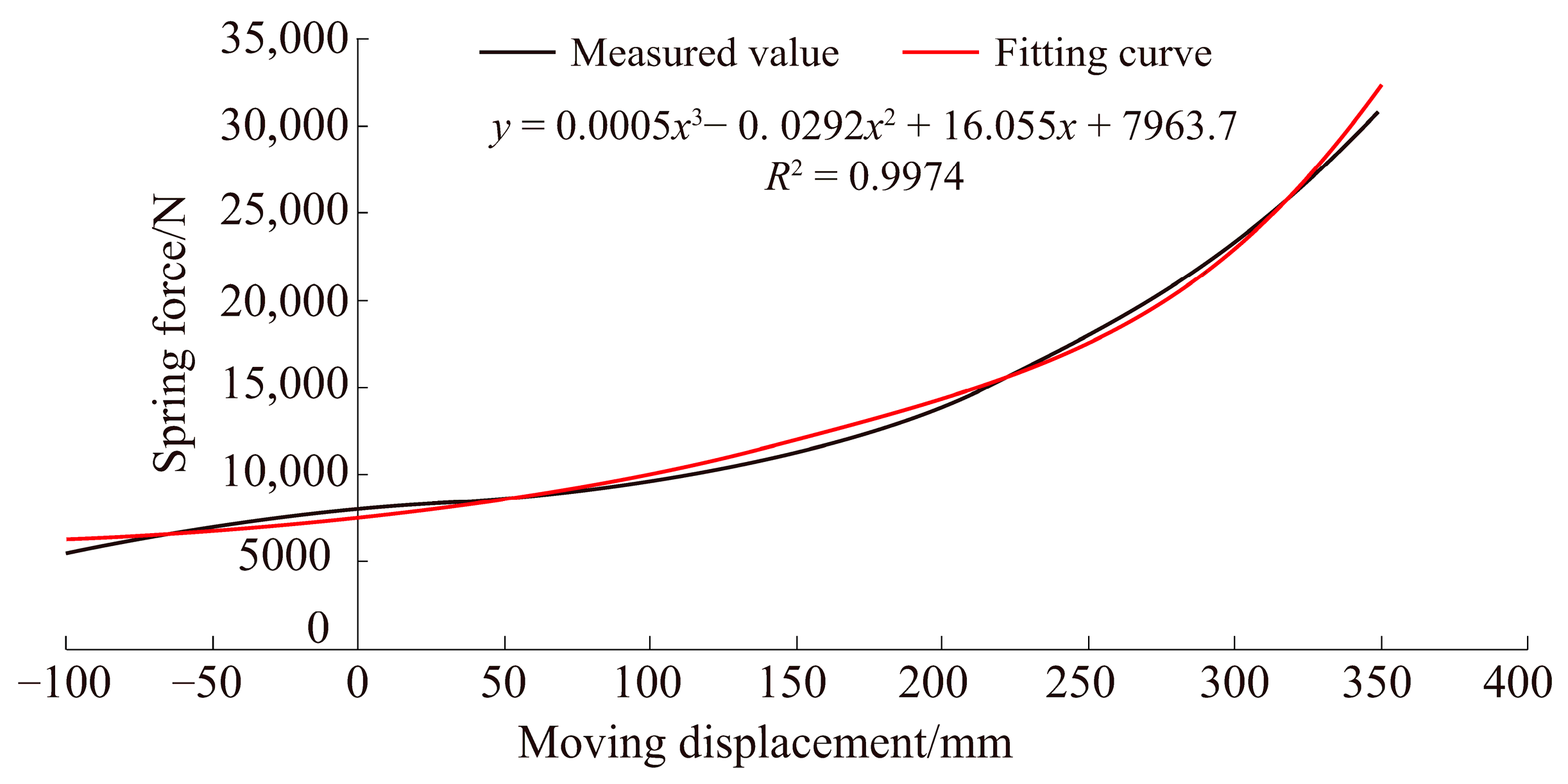
2.2.1. Nonlinear Function Expression

(1)

Nonlinearity of landing gear elastic element

In general, the landing gear spring force increases at an increasing rate as the moving displacement rises, as shown in Figure 2.

Multiple regression analysis is used to examine different fitting models. Considering the fitting effect and the complexity of the formula, a cubic polynomial can be applied to describe the nonlinear characteristics of Figure 2. The fitted formula is shown in Equation (8).

$$F_{\mathrm{s}}=k_{1}x+k_2{x}^2+k_3{x}^3$$

(8)

where $F_{\mathrm{s}}$ is the spring force; $x$ is the moving displacement; and $k_1$, $k_2$, and $k_3$ are fitting parameters.

(2)

Nonlinearity of landing gear damping element

Generally speaking, the damping elements of the landing gear have nonlinear characteristics, which can be expressed by piecewise functions at different velocities, as shown in Equation (9). The relationship curve between the damping force and the moving speed is shown in Figure 3.

$$C\left(x\right)=\{\begin{array}{c}{C}_{3}u\left|u\right|, u<0\\ C_{4}u\left|u\right|, u\ge 0\end{array}$$

(9)

where $C\left(x\right)$ is the damping force; $u$ is the moving speed; and $C_3$ and $C_4$ are fitting parameters.

2.2.2. Calculation of Equivalent Stiffness and Equivalent Damping by Statistical Linearization

In a nonlinear vibration system with n degrees of freedom, the mass of each inertial element is $m_1, m_2,\dots ,m_n$, respectively, and the excitation force $\left\{F\left(t\right)\right\}={\{F_1\left(t\right),F_2\left(t\right),\dots ,F_n\left(t\right)\}}^{\mathrm{T}}$ acting on the system is an n-dimensional joint Gaussian process vector with zero mean. Then, in the inertial coordinate system $y_1,y_2,\dots ,y_n$, the differential equation of motion for this system is shown in Equation (10).

$$\left[M\right]\left\{\ddot{Y}\right\}+\left\{G\left(Y,\dot{Y}\right)\right\}=\left\{F\left(t\right)\right\}$$

(10)

where $\left[M\right]=diag\left[m_i\right]$ is the inertial matrix of the system in the coordinate system $y_1,y_2,\dots ,y_n$; $G\left(Y,\dot{Y}\right)$ is the sum of elastic force and damping force acting on $m_i$; and $F\left(t\right)$ is the exciting force applied to $m_i$.

Suppose the transformation between coordinates $y_1,y_2,\dots ,y_n$ and coordinates $z_1,z_2,\dots ,z_n$ can be expressed as Equation (11).

$$\left\{Y\right\}=\left[A\right]\left\{Z\right\}$$

(11)

Taking Equation (11) into Equation (10), the equation of motion of the system represented by the relative coordinates $z_1,z_2,\dots ,z_n$ is obtained, as shown in Equation (12).

$$\left[M^{\prime }\right]\left\{\ddot{Z}\right\}+\left\{G^{\prime }\left(Z,\dot{Z}\right)\right\}=\left\{F\left(t\right)\right\}$$

(12)

where $\left[M^{\prime }\right]=\left[M\right]\left[A\right]$; and $\left\{G^{\prime }\left(Z,\dot{Z}\right)\right\}=\left\{G^{\prime }\left(Y,\dot{Y}\right)\right\}={[g_1\left(z,\dot{z}\right),g_2\left(z,\dot{z}\right),\dots g_n\left(z,\dot{z}\right)]}^{\mathrm{T}}$.

Assume that the statistically equivalent linear system of the initial nonlinear system satisfies the differential equation shown in Equation (13).

$$\left[M^{\prime }\right]\left\{\ddot{Z}\right\}+\left[C_e\right]\left\{\dot{Z}\right\}+\left[K_e\right]\left\{Z\right\}=\left\{F\left(t\right)\right\}$$

(13)

where $\left[K_e\right]$ and $\left[C_e\right]$ are the equivalent linear stiffness matrix and the equivalent damping matrix, respectively.

$$K_{eij}=E\left[\frac{\partial G_i\left(Z,\dot{Z}\right)}{\partial Z_j}\right], i,j=1,2,\dots ,n$$

(14)

$$C_{eij}=E\left[\frac{\partial G_i\left(Z,\dot{Z}\right)}{\partial {\dot{Z}}_j}\right], i,j=1,2,\dots ,n$$

(15)

Since $f_i\left(Z_i\right)$ is the elastic force of elastic element i, then $d{f}_i\left(Z_i\right)/d{Z}_i$ is the stiffness of elastic element i. Therefore, $E\left[d{f}_i\left(Z_i\right)/d{Z}_i\right]$ should be the statistical equivalent stiffness coefficient $K_{ei}$ of elastic element i, which can be expressed as Equation (15a).

$$K_{ei}=E\left[\frac{d{f}_i\left(Z_i\right)}{d{Z}_i}\right], i=1,2,\dots ,n$$

(15a)

Similarly, the statistically equivalent damping coefficient, $C_{ei}$, of each damping element can be derived as shown in Equation (15b).

$$C_{ei}=E\left[\frac{d{f}_i\left({\dot{Z}}_i\right)}{d{\dot{Z}}_i}\right], i=1,2,\dots ,n$$

(15b)

Consequently, the equivalent stiffness coefficient and the equivalent damping coefficient can be treated as the expected values of Equations (8) and (9) for varying displacement and velocity conditions. In reality, the probability distribution of the vertical vibration displacement of the landing gear and tire during aircraft taxiing becomes relevant. After estimating the probability distribution, Equations (15a) and (15b) can be employed to obtain the statistically equivalent linear coefficient for each element.

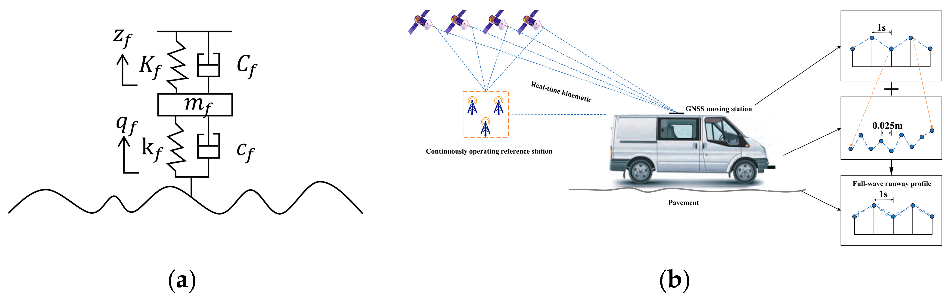
2.3. Pavement Roughness Models

The Federal Aviation Administration (FAA) gathered and published longitudinal profile elevation data for 37 runway centerlines [26]. Our team also collected pavement roughness data for 20 runways in China using a vehicle-mounted laser profile meter and a Beidou high-precision positioning system, which can obtain the true full-wave runway profile [27]. Figure 4 presents the pavement roughness and the data collection system used by our team. The basic information for the 20 Chinese runways collected by our team is presented in

Table 1. Basic information for the 20 Chinese runways.

No.	International Air Transport Association (IATA) Code	Runway Type	Runway Length/m
1	HGH	cement	3560
2	DOY	2/3 asphalt + 1/3 cement	3600
3	WUX	asphalt	3180
4	JGS	cement	2590
5	HYN	cement	2490
6	NGB	cement	3160
7	LCX	cement	2390
8	A military airport	cement	2210
9	A military airport	cement	2280
10	FOC	cement	3580
11	SWA	cement	2480
12	YNZ	cement	2810
13	LFQ	cement	2710
14	A military airport	cement	2990
15	A military airport	cement	2470
16	SHA (runway 1)	cement	3290
17	SHA (runway 2)	asphalt	3290
18	PVG (runway 1)	cement	3410
19	PVG (runway 2)	cement	3770
20	PVG (runway 3)	cement	3390

. Upon analyzing the data, we discovered that asphalt pavement and concrete pavement display distinct digital characteristics in their roughness sequences.

Figure 5 illustrates the power spectrum of measured roughness data for the asphalt pavement (a) at Atlantic City International Airport and the concrete pavement (b) at Taizhou Luqiao Airport. In Figure 5, n is the spatial frequency, and its unit is cycle/m. Dividing n by the unit spatial frequency (1 cycle/m), we can obtain the unitless spatial frequency n_u. Lgn_u is the logarithm of n_u to the base 10. There are notable differences in the power spectrum between asphalt pavement and concrete pavement. The PSD distribution curve of asphalt pavement roughness is relatively smooth, while that of concrete pavement decreases significantly faster at high frequencies. This phenomenon can be attributed to the fact that concrete runways consist of slabs as units, with joints and uneven surfaces between two adjacent slabs, while the surface within a single unit is generally flat. In contrast, asphalt runways are flexible pavements and are relatively more continuous in terms of roughness.

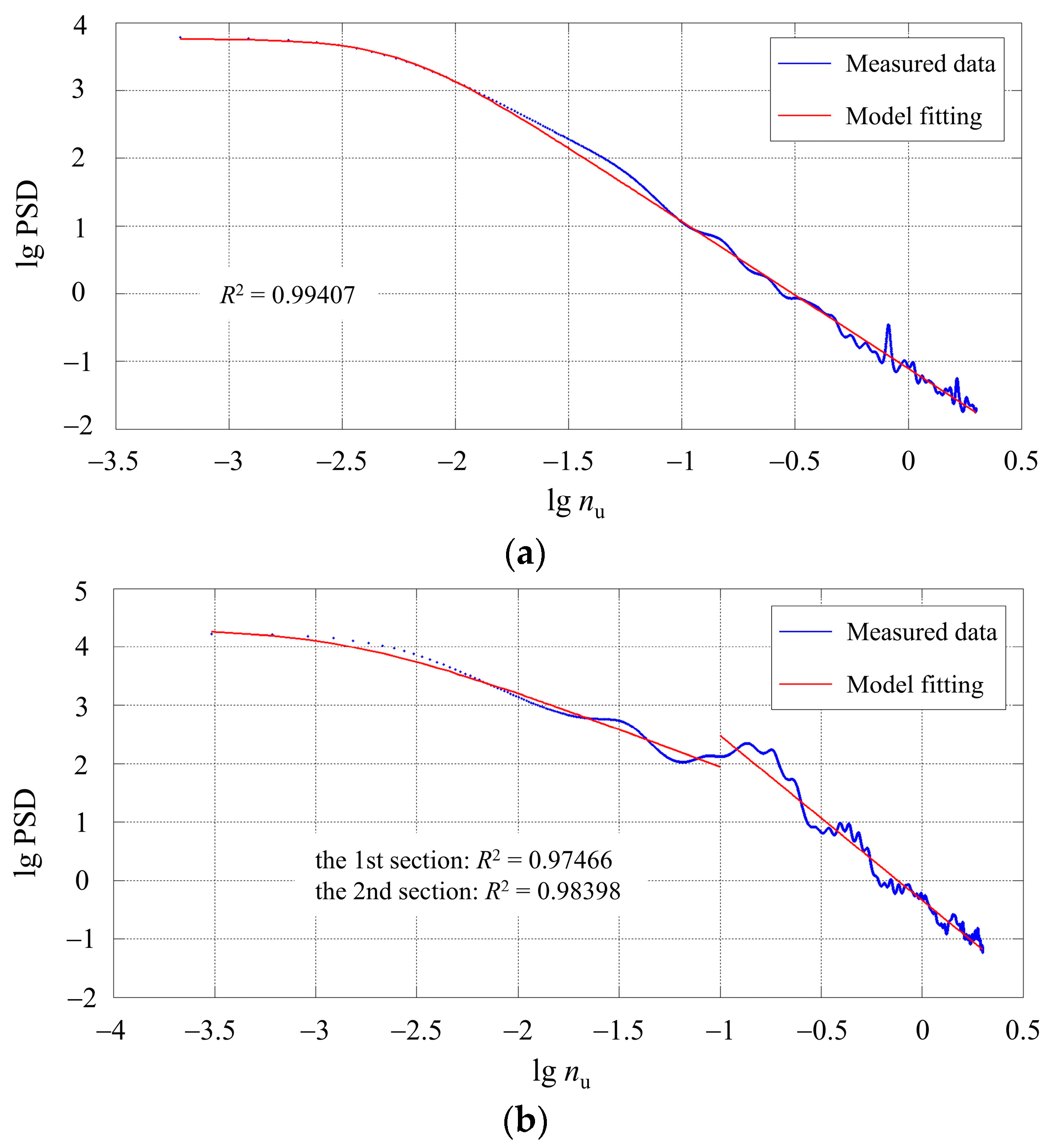
2.3.1. Asphalt Pavement Roughness Model

The roughness power spectrum of 20 asphalt runways, both domestic and international, is analyzed. After repeated comparison, the asphalt pavement roughness model takes reference from the Sussman model [4], as shown in Equation (16).

$$G_{\mathrm{d}}\left(n\right)=\frac{C}{{\alpha }^w+n^w} , 0<n<+\infty$$

(16)

where $G_{\mathrm{d}}\left(n\right)$ is the PSD function of pavement roughness; C is the roughness coefficient, and the larger the C value, the rougher the pavement; w is the frequency index, and the larger w, the more significant the long-wave component; and α is the truncation frequency, and the PSD tends to be smooth as n is less than α.

As Figure 5a shows, the asphalt pavement roughness model established in this paper exhibits a strong fitting effect, with R2 values above 0.95.

2.3.2. Cement Pavement Roughness Model

Since the slab length of concrete runways is generally 5 m, there is an inflection point in the power spectrum curve in Figure 5b around n = 0.1 m⁻¹. By analyzing the roughness power spectrum of 37 concrete runways both domestic and international, this paper utilizes a roughness model with discontinuous segmentation points to represent the concrete pavement, as depicted in Equation (17).

$$G_{\mathrm{d}}\left(n\right)=\{\begin{array}{c}\frac{C_1}{{\alpha }^{w_1}+n^{w_1}} ,n<n_0 \\ \frac{C_2}{n^{w_2}} ,n\ge n_0 \end{array}$$

(17)

where $n_0$ is the segmentation point, $n_0=0.1{ \mathrm{m}}^{-1 }$; $C_1$ and $C_2$ are the roughness coefficients of the first and second sections, respectively; and $w_1$ and $w_2$ are the frequency indexes of the first and second segments, respectively.

As Figure 5b shows, the cement pavement roughness model established in this paper exhibits a strong fitting effect, with R2 values greater than 0.95.

2.3.3. Pavement Roughness Excitation Input

By utilizing the relationship between temporal frequency f, time angular frequency ω, and spatial frequency n (as described in Equations (18a) and (18b)), the pavement roughness model in the spatial domain can be transformed into pavement roughness excitation input in the time domain.

$$f=nv$$

(18a)

$$\omega =2\mathsf{\pi }f$$

(18b)

where v is the aircraft taxiing speed.

The asphalt pavement roughness excitation input in the time domain can be expressed as Equations (19a) and (19b).

$$G_{\mathrm{q}}\left(f\right)=\frac{C}{{\alpha }^{w}v+f^w{v}^{-w+1}} ,0<n<+\infty$$

(19a)

$$G_{\mathrm{q}}\left(\omega \right)=\frac{C}{{\alpha }^{w}2\mathsf{\pi }v+{\omega }^w{(2\mathsf{\pi }v)}^{-w+1}} ,0<n<+\infty$$

(19b)

The cement pavement roughness excitation input in the time domain can be expressed as Equations (20a) and (20b).

$$G_{\mathrm{q}}\left(f\right)=\{\begin{array}{c}\frac{C_1}{{\alpha }^{w_1}v+f^{w_1}{v}^{-w_1+1}} ,n<n_0\\ \frac{C_2}{f^{w_2}{v}^{-w_2+1}} ,n\ge n_0\end{array}$$

(20a)

$$G_{\mathrm{q}}\left(\omega \right)=\{\begin{array}{c}\frac{C_1}{{\alpha }^{w_1}2\mathsf{\pi }v+{\omega }^{w_1}{\left(2\mathsf{\pi }v\right)}^{-w_1+1}} ,n<n_0\\ \frac{C_2}{{\omega }^{w_2}{\left(2\mathsf{\pi }v\right)}^{-w_2+1}} ,n\ge n_0\end{array}$$

(20b)

3. Random Vibration Solution Method

3.1. Solution Method for Steady Random Vibration of Uniform Taxiing Aircraft

Under pavement roughness excitation, the aircraft taxiing at a constant speed generates steady random vibration. To address this, this paper utilizes the PEM to determine the steady vibration response of the aircraft [28]. This method is highly efficient and theoretically accurate, making it widely used in numerous engineering fields [29].

Firstly, the characteristic decomposition of the PSD matrix $\left[S_P\left(f\right)\right]$ of the pavement roughness excitation input is carried out to construct the virtual harmonic excitation, as shown in Equation (21).

$$\left\{{\tilde{P}}_j\left(f,t\right)\right\}=\sqrt{d_j}{\left\{{\phi }_j\right\}}^{*}{e}^{i2\mathsf{\pi }ft}, j=1,2,3.$$

(21)

where $d_j$ is the eigenvalue of matrix $\left[S_p\left(f\right)\right]$; $\left\{{\phi }_j\right\}$ is the eigenvector corresponding to $d_j$; and superscript $*$ represents the conjugate operation.

Secondly, the frequency response function matrix $\left[H\left(f\right)\right]$ of the aircraft system is obtained by the Fourier transform of Equation (7), as shown in Equation (22). Furthermore, the virtual harmonic response ${\tilde{X}}_j\left(f,t\right)$ of the aircraft can be calculated according to Equation (23).

$$\left[H\left(f\right)\right]=\frac{\left[K_{\mathrm{t}}\left]+i2\mathsf{\pi }f\right[C_{\mathrm{t}}\right]}{\left[K_{\mathrm{a}}\right]-4{\mathsf{\pi }}^2{f}^2\left[M_{\mathrm{a}}\left]+i2\mathsf{\pi }f\right[C_{\mathrm{a}}\right]}$$

(22)

$$\left\{{\tilde{X}}_j\left(f,t\right)\right\}=\left[H\left(f\right)\right]\left\{{\tilde{P}}_j\left(f,t\right)\right\}$$

(23)

Finally, the PSD matrix $\left[S_X\left(f\right)\right]$ of the actual aircraft response is solved using Equation (24).

$$\left[S_X\left(f\right)\right]={\displaystyle \sum }_{j=1}^3{\left\{{\tilde{X}}_j\left(f,t\right)\right\}}^{*}{\left\{{\tilde{X}}_j\left(f,t\right)\right\}}^{\mathrm{T}}$$

(24)

where the superscript ^T represents the transpose operation.

Using MATLAB, the vibration response of the aircraft can be solved simply and quickly based on the above steps.

3.2. Solution Method for Non-Stationary Random Vibration of Takeoff and Landing Taxiing Aircraft

In the spatial domain, pavement roughness is steady, but the radial motion of the aircraft during takeoff and landing taxiing is a non-uniform process. As a result, the system differential equation becomes a time-varying differential equation, leading to a non-stationary response of the aircraft system. For a non-stationary random vibration system, the vibration response cannot be calculated directly using the frequency response function H(ω). Therefore, this paper employs the method of instantaneous frequency response function with spatial frequency [30] combined with the PEM to solve the transient power spectrum of the vibration response during aircraft takeoff and landing taxiing.

Lin et al. demonstrated through field measurements and theoretical research that aircraft takeoff and landing taxiing on the runway can be regarded as a uniformly accelerated linear motion process. The corresponding velocity v and displacement s can be expressed as described in Equations (25a) and (25b) [31].

$$v=v_0+at$$

(25a)

$$s=v_{0}t+a{t}^2/2$$

(25b)

where $v_0$ is the initial velocity of uniform variable motion, which is taken as 0 during the aircraft takeoff taxiing, and the landing speed during aircraft landing taxiing; a is the acceleration, which is positive during the aircraft takeoff taxiing and negative during the aircraft landing taxiing.

The time–space frequency relationship of the uniformly varying motion during aircraft takeoff and landing taxiing can be obtained by substituting Equations (25a) and (25b) into Equation (18), as shown in Equation (26).

$$f=nv=n\sqrt{\left(v_0^2+2as\right)}$$

(26)

Based on the characteristic that the frequency response function H(ω) of the aircraft system in non-stationary random vibration is constant at temporal frequency, the instantaneous frequency response function $H\left(n,t\right)$ at spatial frequency can be derived from the relationship between temporal frequency and spatial frequency. Therefore, by substituting Equation (26) into Equation (22), the instantaneous spatial domain frequency response function matrix of the aircraft system can be expressed as Equation (27).

$$H\left(n,t\right)=\frac{\left[K_{\mathrm{t}}\right]+i2\mathsf{\pi }n\sqrt{\left(v_0{}^2+2as\right)}\left[C_{\mathrm{t}}\right]}{\left[K_{\mathrm{a}}\right]-4{\mathsf{\pi }}^2{n}^2\left(v_0{}^2+2as\right)\left[M_{\mathrm{a}}\right]+i2\mathsf{\pi }n\sqrt{\left(v_0{}^2+2as\right)}\left[C_{\mathrm{a}}\right]}$$

(27)

After obtaining Equation (27), the instantaneous spatial PSD of the aircraft vibration response can be calculated following the PEM in Section 3.1.

4. Application Scenarios

4.1. Aircraft Parameters

In this paper, the B737-800 is selected as the representative model. Based on the values given in

Table 2. Parameters of representative aircraft.

Parameter	Unit	Value	Description
Ms (Taxiing)	kg	78,472	sprung mass
Ms (Takeoff)	kg	78,245	sprung mass
Ms (Landing)	kg	65,317	sprung mass
mf	kg	578	unsprung mass of front landing gear
ml	kg	1150	unsprung mass of left rear landing gear
mr	kg	1150	unsprung mass of right rear landing gear
Kf	N/m	58,027	stiffness coefficient of front landing gear buffer
Kl	N/m	996,531	stiffness coefficient of left rear landing gear buffer
Kr	N/m	996,531	stiffness coefficient of right rear landing gear buffer
kf	N/m	1,966,300	stiffness coefficient of front landing gear tire
kl	N/m	2,812,900	stiffness coefficient of left rear landing gear tire
kr	N/m	2,812,900	stiffness coefficient of right rear landing gear tire
Cf	N·s/m	131,500	damping coefficient of front landing gear buffer
Cl	N·s/m	572,500	damping coefficient of left rear landing gear buffer
Cr	N·s/m	572,500	damping coefficient of right rear landing gear buffer
cf	N·s/m	131,500	damping coefficient of front landing gear tire
cl	N·s/m	4066	damping coefficient of left rear landing gear tire
cr	N·s/m	4066	damping coefficient of right rear landing gear tire
Ix	kg·m2	3,394,953	rotational inertia of aircraft around x-axis
Iy	kg·m2	1,866,711	rotational inertia of aircraft around y-axis
a	m	2.86	horizontal distance from left landing gear to y-axis
b	m	2.86	horizontal distance from right landing gear to y-axis
d	m	14.6	horizontal distance from front landing gear to x-axis
e	m	1	horizontal distances from rear landing gear to x-axis

, the equivalent linear stiffness coefficient for the nose landing gear is 58,027 N/m and the equivalent linear damping coefficient is 131,500 N·s/m. The equivalent linear stiffness coefficient for the main landing gear is 996,531 N/m and the equivalent linear damping coefficient is 572,500 N·s/m.

4.2. Pavement Roughness Parameters

The power spectrum of the measured data from the 57 runways is fitted using the asphalt and cement pavement roughness models developed in this paper. The distributions of the fitting parameters for asphalt and cement pavements are presented in

Table 3. Asphalt pavement fitting parameters’ distribution.

Runways	C	$\mathit{\alpha }$	w
2 runways in China	0.0907~0.119 (0.1)	0.00054~0.0014 (0.0009)	2.199~2.285 (2.24)
18 runways abroad	0.0227~1.206 (0.1)	0.00019~0.00178 (0.0005)	2.042~3.162 (2.3)

and

Table 4. Cement pavement fitting parameters’ distribution.

Runways	C1	$\mathit{\alpha }$	w1
18 runways in China	0.0089–0.235 (0.025)	0.00009–0.1503 (0.04)	1.369–3.527 (2.4)
19 runways abroad	0.007–0.147 (0.025)	0.0000152–0.0103 (0.005)	1.21–3.22 (2.5)
Runways	C2	w2
18 runways in China	0.049–0.597 (0.08)	1.813–3.13 (2.5)
19 runways abroad	0.029–0.308 (0.08)	1.59–2.86 (2.2)

, respectively. The values in brackets in the tables are the parameter values at the maximum probability density, i.e., the typical asphalt pavement and cement pavement roughness parameters. In order to increase the representativeness of the study, typical roughness parameters of domestic runways for both asphalt and cement pavements are employed.

5. Results and Discussion

5.1. Vibration Response Analysis of Aircraft Taxiing under Different Pavement Types

The PSD distributions of CGA, PSA, NGDLC, and MGDLC under typical roughness excitations of both asphalt pavement and concrete pavement during a 100 km/h taxiing of a B737-800 aircraft are shown in Figure 6a to Figure 6d, respectively. Overall, the PSD distribution of each vibration response is similar for both pavement types, as shown in Figure 6. The red and black lines show a similar trend of rising and falling, and the sensitivity frequencies corresponding to each peak are almost the same. However, the vibration response corresponding to concrete pavement roughness at around 2.6 Hz decreases dramatically. This is attributed to the segmental characterization of the concrete pavement roughness model, which has few broken slabs or cracks within the concrete slab and high flatness.

5.2. Vibration Response Analysis of Aircraft Taxiing under Different Motion Attitudes

The runway takeoff distance is set at 2500 m, and the B737-800 aircraft takes off from the ground at a speed of 260 km/h with an acceleration of 1.04 m/s² throughout the process. The PSD distributions of CGA, PSA, MGDLC, and NGDLC under typical asphalt pavement roughness excitation during takeoff are shown in Figure 7a–d. The power spectral density distribution of the system response at any instant on the runway is consistent with the uniform steady-state response. As the takeoff distance increases, the taxiing speed of the aircraft increases, and the PSD of the vibration response generally increases, although not monotonically. For example, the PSD of CGA is locally reduced near the airframe resonance frequency within the distance range of 1000–1500 m. The most sensitive frequency of the aircraft remains unchanged in each spatial segment, which is due to the constant natural frequency of the aircraft structure.

The landing speed of the B737-800 is set at 220 km/h, the landing distance is set at 1000 m, and the acceleration is −1.86 m/s². The PSD distributions of CGA, PSA, MGDLC, and NGDLC under typical asphalt pavement roughness excitation during landing are shown in Figure 8a–d. In general, the closer to the landing site, the greater the PSD of the vibration response. Thus, during the landing process, the first half of the runway roughness has a stronger impact on the aircraft vibration. Compared to the takeoff process, the PSD of the aircraft vibration response during landing is greater because the aircraft’s mass decreases due to fuel consumption during the flight, and the aircraft’s acceleration during landing deceleration is larger. Therefore, the roughness of the landing runway should be of greater concern to managers than that of the takeoff runway.

5.3. Vibration Response Analysis of Aircraft Taxiing under Stochastic Structural Parameters

Due to the large number of degrees of freedom in the aircraft model, it is complicated to theoretically derive the effect of stochastic structural parameters on the vibration response. The Monte Carlo method can build a mathematical model of the input and output variables, apply the probability distribution of each variable to random sampling, and calculate the output variables using the randomly generated input variables. By repeating the random simulations, the probability distribution function of a certain output variable can be obtained. Additionally, the accuracy of the output variable’s probability distribution function increases with the number of simulations. With the aid of the MATLAB (R2019a) software and the Monte Carlo method, this paper analyzes the variation in each vibration response when the probability density function of aircraft structural parameters is modeled as a normal distribution.

The variation coefficients of the sprung mass, rotational inertia, stiffness coefficient of the landing gear buffer, damping coefficient of the landing gear buffer, stiffness coefficient of the tire, and damping coefficient of the tire are all set to 0.05. By using the Monte Carlo method to randomly sample 1000 times at a time, the variation coefficient distribution of the variance of CGA, PSA, NGDLC, and MGDLC can be obtained, as shown in Figure 9.

The influence of the sprung mass is the largest, having a significant effect on the four vibration responses, with variation coefficient values exceeding 0.05. Among them, the sprung mass has the greatest impact on NGDLC, reaching 0.113. The rotational inertia mainly affects PSA, with variation coefficients above 0.05, but has little effect on the other three vibration responses. The damping coefficient of the landing gear buffer has a greater impact than the stiffness coefficient of the landing gear buffer. The damping coefficient of the front landing gear affects PSA and NGDLC more, while the damping coefficient of the main landing gear has a greater impact on CGA and MGDLC, as the center of gravity is closer to the main landing gear. The situation with the tire is the opposite of that of the landing gear, with the tire damping coefficient having a much smaller effect than the tire stiffness. The stiffness coefficient of the tire has a great influence on the dynamic load coefficient of the landing gear where it is located, but it has little effect on the other landing gear. At the same time, the stiffness coefficient of the main landing gear tire has a greater impact on the fuselage vibration than the front landing gear, indicating that more attention should be paid to the roughness excitation applied to the main landing gear.

6. Conclusions

In this paper, pavement roughness models for both asphalt and cement pavements are established based on their structural characteristics. The PEM, the method of instantaneous frequency response function with spatial frequency, and the Monte Carlo method are used to comprehensively analyze the influence of different pavement types, different motion attitudes, and stochastic structural parameters on the vibration response of a 6-DOF aircraft model under random roughness excitation in the frequency domain. The results of the study can be adopted for runway roughness evaluation and aircraft structure design. The main conclusions from this study are as follows:

(1)

The power spectra of asphalt pavement and cement pavement roughness are different. The corresponding pavement roughness models were developed in this paper and the measured data demonstrates that the fit is excellent, with R2 values greater than 0.95.

(2)

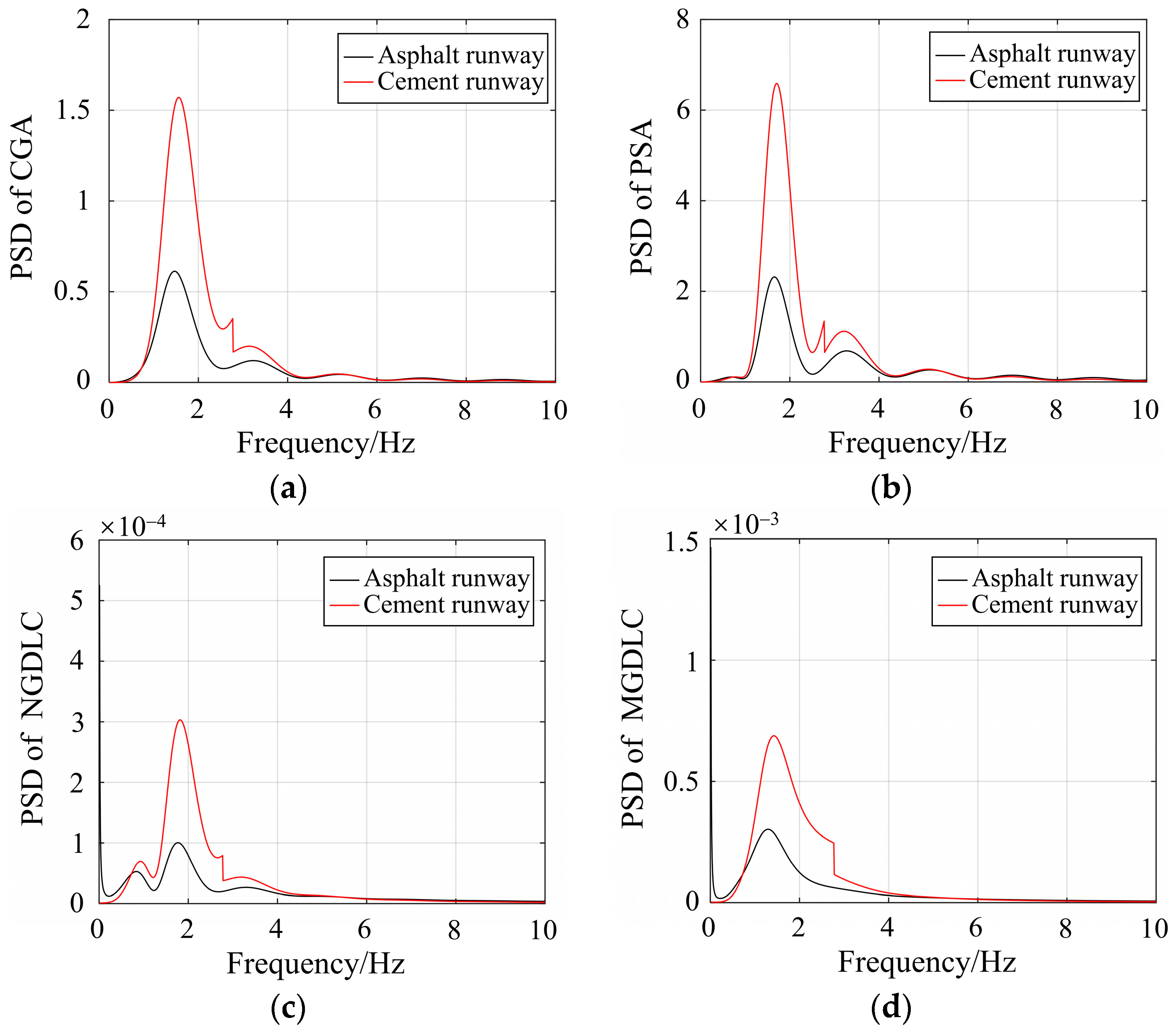
The pavement type has little influence on the PSD distribution of the aircraft vibration response. When the accuracy requirements are not high, the same pavement roughness model can be used for both cement and asphalt pavements.

(3)

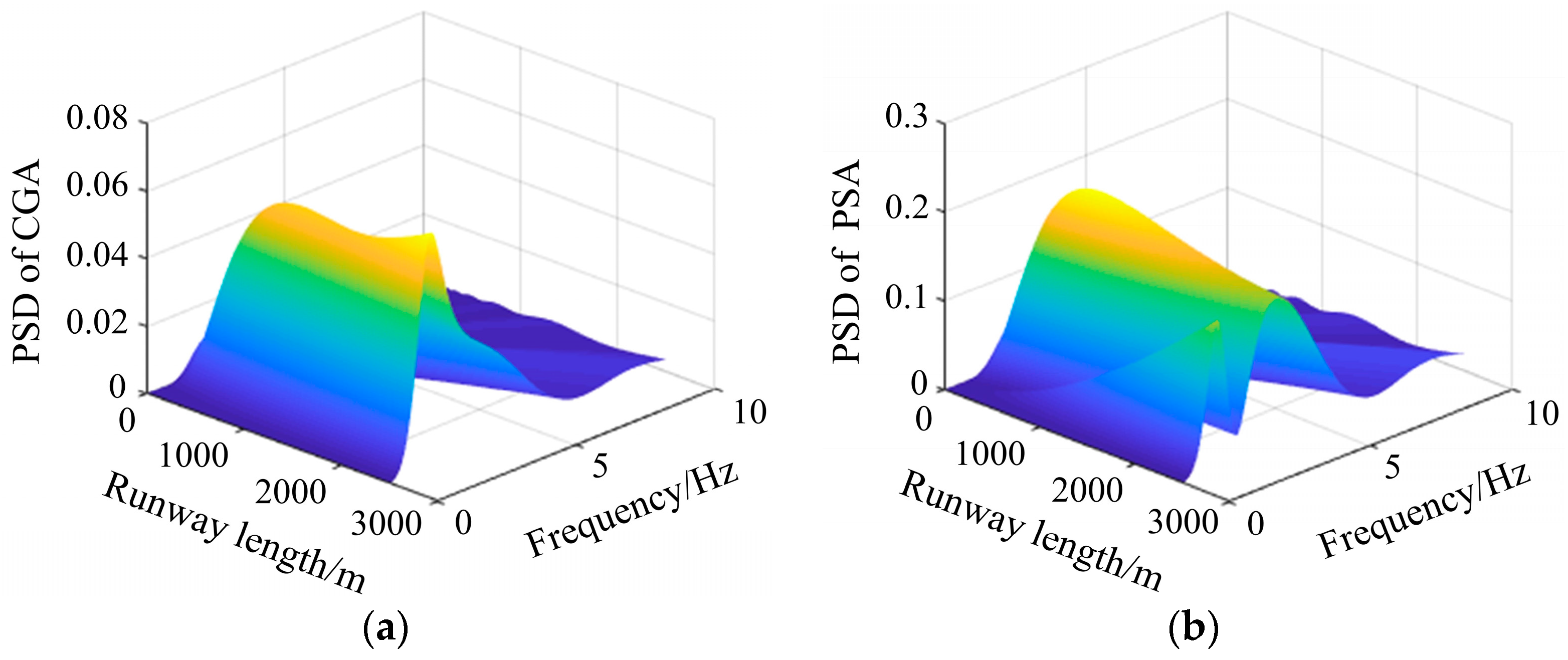
The vibration response of the aircraft during landing is greater than that during takeoff under the same conditions. Managers should therefore pay more attention to the roughness of the landing runway compared to the takeoff runway.

(4)

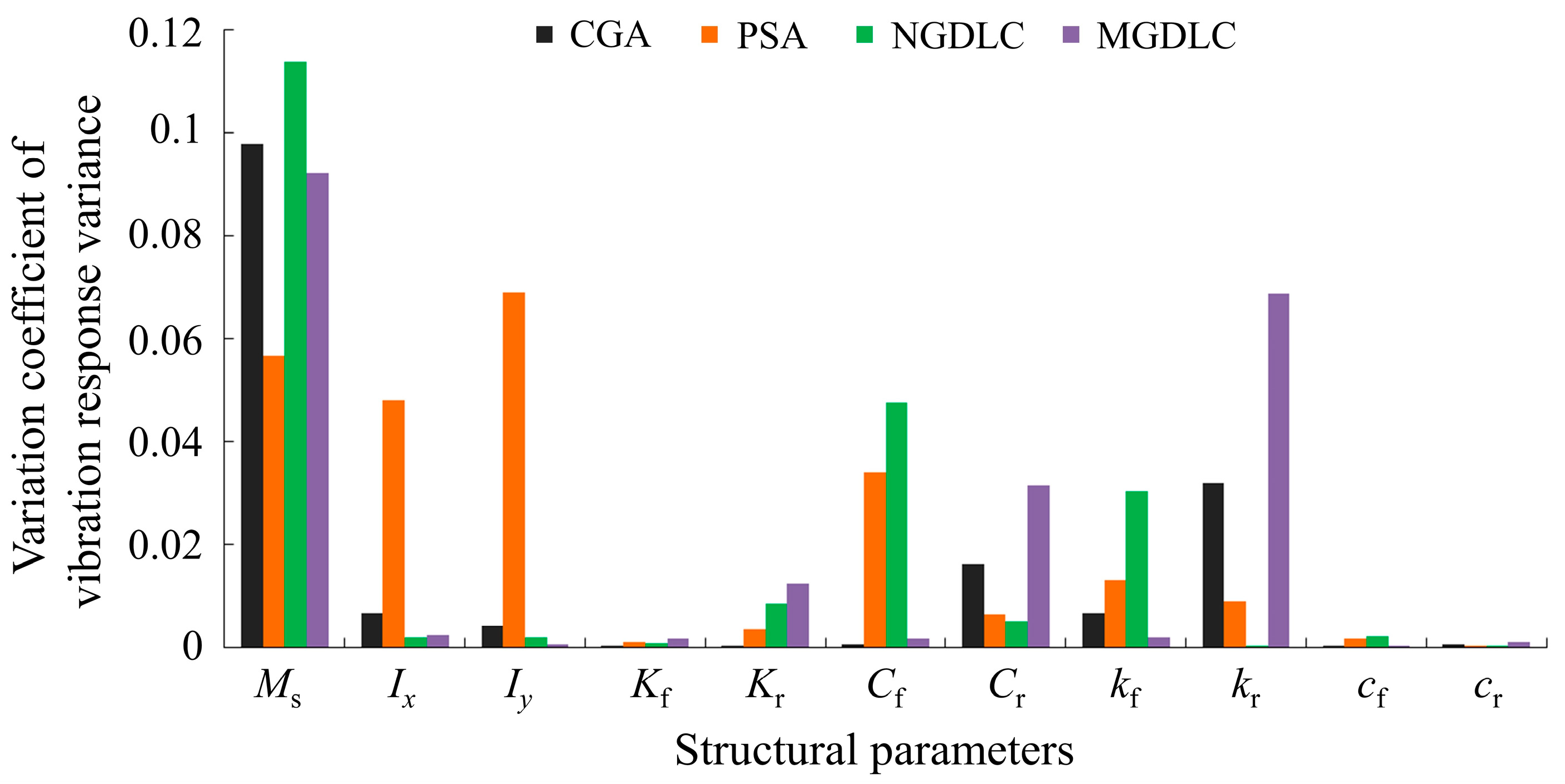
The impact of stochastic structural parameters on the aircraft’s vibration response was analyzed using the Monte Carlo method. It was found that the randomness of the sprung mass has the greatest effect on the vibration response and can result in NGDLC reaching 0.113, followed by the tire stiffness and the aircraft’s rotational inertia.

References

1. Loprencipe, G.; Zoccali, P. Comparison of methods for evaluating airport pavement roughness. Int. J. Pavement Eng. 2019, 20, 782–791. [Google Scholar] [CrossRef]
2. Andren, P. Power spectral density approximations of longitudinal road profiles. Int. J. Veh. Des. 2006, 40, 2–14. [Google Scholar] [CrossRef]
3. Dodds, C.J.; Robson, J.D. The description of road surface roughness. J. Sound Vib. 1973, 31, 175–183. [Google Scholar] [CrossRef]
4. Sussman, N.E. Statistical ground excitation models for high speed vehicle dynamic analysis. High Speed Ground Transp. J. 1974, 8, 145–154. [Google Scholar]
5. Gillespie, T.D. Heavy Truck Ride; Society of Automotive Engineers: Warrendale, PA, USA, 1985. [Google Scholar]
6. Marcondes, J.; Burgess, G.J.; Harichandran, R.; Snyder, M.B. Spectral analysis of highway pavement roughness. J. Transp. Eng. 1991, 117, 540–549. [Google Scholar] [CrossRef]
7. Xu, D.M.; Mohamed, A.M.O.; Yong, R.N.; Caporuscio, F. Development of a criterion for road surface roughness based on power spectral density function. J. Terramech. 1992, 29, 477–486. [Google Scholar] [CrossRef]
8. Houbolt, J.C. Runway roughness studies in the aeronautical field. Am. Soc. Civ. Eng. Trans. 1962, 127, 427–447. [Google Scholar] [CrossRef]
9. Sivakumar, S.; Haran, A.P. Mathematical model and vibration analysis of aircraft with active landing gears. J. Vib. Control 2015, 21, 229–245. [Google Scholar] [CrossRef]
10. Sivakumar, S.; Selvakumaran, T.; Sanjay, B. Investigation of random runway effect on landing of an aircraft with active landing gears using nonlinear mathematical model. J. Vibroengineering 2021, 23, 1785–1799. [Google Scholar] [CrossRef]
11. Ling, D.S.; Sheng, W.J.; Huang, B. Influence of pavement unidirectional constraint on aircraft vibration response. J. Zhejiang Univ. Eng. Sci. 2021, 55, 1684–1693. [Google Scholar]
12. Li, S.; Guo, J. Modeling and dynamic analysis of an aircraft–pavement coupled system. J. Vib. Eng. Technol. 2022, 1–13. [Google Scholar] [CrossRef]
13. Ling, J.M.; Liu, S.F.; Yuan, J.; Lei, X.P. Comprehensive analysis of pavement roughness evaluation for airport and road with different roughness excitation. J. Tongji Univ. Nat. Sci. 2017, 45, 519–526. [Google Scholar]
14. Durán, J.B.C.; Júnior, J.L.F. Airport pavement roughness evaluation based on cockpit and center of gravity vertical accelerations. Transportes 2020, 28, 147–159. [Google Scholar] [CrossRef]
15. Dong, Q.; Wang, J.H.; Zhang, X.M. Vibration response of rigid runway under aircraft-runway coupling. J. Vib. Shock 2021, 40, 64–72. [Google Scholar]
16. Cheng, G.Y.; Hou, D.W.; Huang, X.D. Pavement roughness limit value standard based on aircraft vertical acceleration. J. Vib. Shock 2017, 36, 166–171. [Google Scholar]
17. Shi, X.G.; Cai, L.C.; Wang, G.H.; Liang, L. A new aircraft taxiing model based on filtering white noise method. IEEE Access 2020, 8, 10070–10087. [Google Scholar] [CrossRef]
18. Liu, S.F.; Tian, Y.; Liu, L.; Xiang, P.; Zhang, Z.K. Improvement of Boeing Bump method considering aircraft vibration superposition effect. Appl. Sci. 2021, 11, 2147. [Google Scholar] [CrossRef]
19. Qian, J.S.; Pan, X.W.; Cen, Y.B.; Liu, D.L. Aircraft taxiing dynamic load induced by runway roughness. J. Vib. Shock 2022, 41, 176–184+269. [Google Scholar]
20. Kirk, C.L.; Perry, P.J. Analysis of taxiing induced vibrations in aircraft by the power spectral density method. Aeronaut. J. 1971, 75, 182–194. [Google Scholar] [CrossRef]
21. Tung, C.C. The effects of runway roughness on the dynamic response of airplanes. J. Sound Vib. 1967, 5, 164–172. [Google Scholar] [CrossRef]
22. Nie, H.; Kortum, W. Analysis for aircraft taxiing at variable velocity on unevenness runway by the power spectral density method. Trans. Nanjing Univ. Aeronaut. Astronaut. 2000, 17, 64–70. [Google Scholar]
23. Wang, C.Q. Dynamic response analysis of UAV’s landing gear structure subjected to random excitation. Comput. Simul. 2014, 31, 69–72+460. [Google Scholar]
24. Liu, S.F.; Ling, J.M.; Tian, Y.; Hou, T.X.; Zhao, X.D. Random vibration analysis of a coupled aircraft/runway modeled system for runway evaluation. Sustainability 2022, 14, 2815. [Google Scholar] [CrossRef]
25. Liu, S.F.; Tian, Y.; Yang, G.; Ling, J.M.; Li, P.L. Effect of space for runway roughness evaluation. Int. J. Pavement Eng. 2022, 1–11. [Google Scholar] [CrossRef]
26. Federal Aviation Administration. Surface Roughness Final Study Data Collection Report; Federal Aviation Administration: Washington, DC, USA, 2014.
27. Qian, J.S.; Cen, Y.B.; Liu, D.L.; Li, J.S.; Liu, S.F. Measurement method of all-wave airport runway roughness. J. Traffic Transp. Eng. 2021, 21, 84–93. [Google Scholar]
28. Lin, J.H.; Zhang, Y.H. Pseudo Excitation Method in Random Vibration; Science Press: Beijing, China, 2004. [Google Scholar]
29. Lin, J.H.; Zhang, Y.H.; Zhao, Y. The pseudo-excitation method and its industrial applications in China and abroad. Appl. Math. Mech. 2017, 38, 1–31. [Google Scholar]
30. Zhang, L.J.; He, H.; Wang, Y.S. Analysis on instantaneous spatial spectrum of vehicle response. J. Vib. Shock 2003, 22, 16–20. [Google Scholar]
31. Lin, K.X.; Cen, G.P.; Li, L.; Liu, G. Simulation and analysis for airplanes performance of takeoff and landing. J. Air Force Eng. Univ. Nat. Sci. Ed. 2012, 13, 21–25. [Google Scholar]
Figure 1. Ground dynamics model of a 6-DOF aircraft: (a) The overall diagram of the ground dynamics model of a 6-DOF aircraft; (b) local diagram of the ground dynamics model of a 6-DOF aircraft.
Applsci 13 07386 g001
Figure 2. Variation curve of landing gear spring force with moving displacement.
Applsci 13 07386 g002
Figure 3. Variation curve of landing gear damping force with moving speed.
Applsci 13 07386 g003
Figure 4. Pavement roughness and data collection: (a) Pavement roughness; (b) data collection.
Applsci 13 07386 g004
Figure 5. Power spectrum and roughness model of measured data of asphalt and cement pavement: (a) Atlantic City International Airport (asphalt pavement); (b) Taizhou Luqiao Airport (cement pavement).
Applsci 13 07386 g005
Figure 6. PSD distribution of vibration response under different pavement types: (a) PSD distribution of CGA; (b) PSD distribution of PSA; (c) PSD distribution of NGDLC; (d) PSD distribution of MGDLC.
Applsci 13 07386 g006
Figure 7. PSD distribution of vibration response during takeoff: (a) PSD distribution of CGA; (b) PSD distribution of PSA; (c) PSD distribution of MGDLC; (d) PSD distribution of NGDLC.
Applsci 13 07386 g007aApplsci 13 07386 g007b
Figure 8. PSD distribution of vibration response during landing: (a) PSD distribution of CGA; (b) PSD distribution of PSA; (c) PSD distribution of MGDLC; (d) PSD distribution of NGDLC.
Applsci 13 07386 g008
Figure 9. Variation coefficient of vibration response variance under random structural parameters.
Applsci 13 07386 g009