Article

Dynamic Modeling of Flue Gas Desulfurization Process via Bivariate EMD-Based Temporal Convolutional Network

Faculty of Information Technology, Beijing University of Technology, Beijing 100124, China
*
Author to whom correspondence should be addressed.
Appl. Sci. 2023, 13(13), 7370; https://doi.org/10.3390/app13137370
Submission received: 23 May 2023 / Revised: 14 June 2023 / Accepted: 19 June 2023 / Published: 21 June 2023

Abstract

:
Sulfur dioxide (SO2) can cause detrimental impacts on the ecosystem. It is well known that coal-fired power plants play a dominant role in SO2 emissions, and consequently industrial flue gas desulfurization (IFGD) systems are widely used in coal-fired power plants. To remove SO2 effectively such that ultra-low emission standard can be satisfied, IFGD modeling has become urgently necessary. IFGD is a chemical process with long-term dependencies between time steps, and it typically exhibits strong non-linear behavior. Furthermore, the process is rendered non-stationary due to frequent changes in boiler loads. The above-mentioned properties make IFGD process modeling a truly formidable problem, since the chosen model should have the capability of learning long-term dependencies, non-linear dynamics and non-stationary processes simultaneously. Previous research in this area fails to take all the above points into account at a time, and this calls for a novel modeling approach so that satisfactory modeling performance can be achieved. In this work, a novel bivariate empirical mode decomposition (BEMD)-based temporal convolutional network (TCN) approach is proposed. In our approach, BEMD is employed to generate relatively stationary processes, while TCN, which possesses long-term memory ability and uses dilated causal convolutions, serves to model each subprocess. Our method was validated using the operating data from the desulfurization system of a coal-fired power station in China. Simulation results show that our approach yields desirable performance, which demonstrates its effectiveness in the IFGD dynamic modeling problem.

1. Introduction

It is well known that SO2 present in the flue gas from coal-fired power plants can cause health hazards and have an adverse effect on environment. In coal-fired power plants, the flue gas desulfurization process is set up to remove SO2 in raw boiler flue gas, and hence the study of IFGD modeling is of great significance to environmental protection [1], SO2 emission control [2], and system optimization [3]. However, the IFGD is a non-stationary process with high time delay and highly non-linear dynamics, which makes it rather challenging to model it using traditional modeling techniques. To overcome this difficulty, a novel modeling approach is proposed in our research. The IFGD modeling problem has raised great concern among many countries, such as Sweden [4], China [5,6], Poland [7] and Britain [8].
The ever-increasing demand for power energy naturally calls for significant amounts of coal consumption, which in turn leads to massive flue gas emissions. The high content of SO2 in flue gas brings about an adverse impact on environment and human health, rendering the flue gas desulfurization particularly necessary. In fact, the primary source of SO2 in atmosphere stems from coal combustion in thermal power stations, which accounts for about 70% of China’s total SO2 emissions [9,10]. As a consequence, Chinese government have placed stringent regulation on SO2 emissions and requested that the SO2 concentration of outlet flue gas should be lower than 35 mg/m3 [11]. In response to the above problems, the wet IFGD technique, as the most mature and reliable SO2 removal technology, is widely applied in coal-fired plants power stations worldwide. In view of the above considerations, it is of great significance to fully capture the complex dynamics of an IFGD process, in a way that the resulting identification model can provide precise information on key variables therein.
Over the past few decades, considerable numbers of studies have been conducted on this problem, and modeling approaches can broadly be classified into two categories: first-principles models and data-driven models. For the former, the chemistry and reaction within the overall desulfurization process should be considered, and gas–liquid mass transfer theory is typically utilized to identify the IFGD process. On the basis of the penetration theory, an IFGD model that characterizes instantaneous equilibrium reactions is developed in [4], and have been applied successfully for the calculation of SO2 absorption rate. In [12], the liquid side mass transfer during absorption of SO2 is studied and utilized to build flux equations, based upon which the SO2 absorption rate can be readily calculated. More recently, for a full-scale IFGD system, mass transfer and reaction during the oxidation process is studied in detail in [5], and a mechanism-based model characterized by good interpretability and robustness was developed. The study in [13] combined chemical mechanisms for desulfurization with the Eulerian–Eulerian two-phase/porous media model, and conducted a series of numerical investigations for fluid mechanics in the desulfurization tower. In contrast to first-principles models, data-driven models are developed purely dependent on operating measurements and thus more easily implementable. In spite of this fact, there is a lack of studies on the data-driven approach in this direction, and artificial neural network (ANN) is typically the prime candidate for IFGD process modeling purposes. To find optimum operating ranges of key variables in the IFGD process, multilayer perceptron-based models were first established in [14] to map the non-linear and causal relationships between nine input variables and four output variables, then Monte Carlo experiments along with statistical analysis were performed based on developed models, and corresponding conclusions are drawn. ANNs were employed in [6] to build the mathematical relationship among different IFGD variables, which then serves as the objective function in the formulated optimization problem. With the aid of the function approximation capability of the ANN model, the issue of optimized operation in IFGD is well addressed. Likewise, in [7], neural model was successfully applied to calculate SO2 emissions in an IFGD context; experimental results show its validity by comparing with the simplified first-principle model. Other applications of the ANN in the area of IFGD process modeling can be found in [15,16], where back propagation-based network and extreme learning machine methods are used, respectively. Despite the IFGD process having an inherent nonlinearity, linear parametric models are frequently used for problem simplification purposes. For instance, in [8], based on a standard logistic diffusion equation, a linear regression model was built to describe the evolution of flue gas diffusion over time. Choosing desulfurization as the predicted variable, while slurry flow rate and inlet SO2 concentration as exploratory variables, a quadratic regression model is employed in [17] to establish the mapping between above the variables. According to the results of analysis of variance (ANOVA), the established model performed well in fitting.
Considering the high complexity of chemical reactions in the IFGD process, we focus exclusively on the data-driven modeling approach in this study. It is found that a common characteristic of the above-mentioned linear or non-linear models is that they are all memoryless, namely dynamic characteristics of the process are not taken into account. Lack of dynamics characterization is only one of research gaps in the literature; other gaps include the following: (1) large time delay in IFGD process, and (2) the non-stationary property brought by boiler load fluctuations, which are not considered in the modeling process. This work proposes a novel dynamic modeling approach to fill in the above-mentioned gaps, and the main contribution of this paper can be concluded as follows.
  • For the first time, bivariate EMD is used for process identification purposes, which can lower the non-stationary degree and simplify frequency components of the original process, in such a way that the process is more readily identified.
  • TCN, which has the capability of learning long-term dependencies between time steps, is innovatively employed in the process identification field. In this work, it serves to model each intrinsic mode function (IMF) as well as residue, and the final modeling result is obtained by summing up all the identified subprocesses.
  • Combination of signal processing technique and deep learning model are for the first time used successfully in an IFGD modeling problem.
The FGD process is briefly described and the identification problem is formulated mathematically in Section 2. Thereafter, in Section 3, our proposed method is described in detail. Section 4 deals with simulation studies in a practical desulfurization context, where the performance of our method is compared with commonly used ones, and finally relevant conclusions are drawn in Section 5.

2. Description of IFGD Process and Modeling Problem

In this section, we provide a brief introduction of the IFGD process which is the background of our modeling problem. Then, details of the modeling problem under study are given and discussed.

2.1. Limestone Wet IFGD Process

Limestone wet flue gas desulfurization, with the property of high SO2 removal efficiency, rapid reaction speed and operating reliability, has become the most widely used IFGD technology worldwide [18]. In the limestone wet IFGD process, the SO2-containing flue gas reacts with limestone reagent slurry (CaCO3), along with injected oxygen (O2); the intermediate product is calcium sulfite (CaSO3), and the final product gypsum (CaSO4) is produced. The above procedure can be expressed in a chemical reaction form,
SO 2 + CaCO 3 ( s ) CaSO 3 + CO 2
CaCO 3 + 0.5 O 2 CaSO 4 ( s )
To further explain the IFGD process, Figure 1 shows a schematic of the overall desulfurization process. Having processed by electrostatic precipitator and heat exchanger, the cool and cleaned flue gas enters from the lower part of the spray tower. The entered flue gas is bottom-up, while the slurry is pumped from the reaction tank to spray headers and moves from up to bottom. In such a countercurrent contact, reactions (1) and (2) take place and gypsum is produced as one of reaction products. Then, the gypsum byproduct is transferred to the dehydration system for further processing, which mainly includes gypsum separation and dehydration with hydrocyclone and vacuum dehydrator, respectively. Lastly, the desulfurized flue gas is emitted from the stack after water elimination.
Limestone flow rate, as the input variable of IFGD process in our study, is measured via the flowmeter installed on the duct between the slurry pump and the slurry tank in the absorber (see Figure 1), which can record the flow rate of limestone slurry in real time. On the other hand, pH meter, which is installed on the duct between circulating pump and spray headers, is used to measure the pH value of the circulating slurry (see Figure 1).

2.2. Description of IFGD Process and Modeling Problem

The IFGD process under study is an inherently non-linear dynamic process, and dynamics involved in it is quite complicated even though the overall reaction shown in (1) is simple. The distinct nonlinearity in FGD process stems from the dynamics of thermodynamic relations, chemical reactions, etc. Furthermore, long time delay is often involved in a lot of industrial processes, due to mass transportation, energy exchange and so on [19,20]. As for the IFGD process under study, the time delay mainly arises from slurry flow through pipes. Empirically, it is found that the time delay in our process is approximately half an hour, which makes FGD modeling really a challenging problem in the field of system identification. In an IFGD process, both desulfurization efficiency and gypsum quality are critically dependent upon the pH of absorber slurry; on the other hand, the slurry flow has a direct influence on the pH value. In this sense, the input and output of the process are chosen as slurry flow (m3/h) and pH in absorber slurry, respectively. Let the IFGD process be described by the following single-input single-output (SISO) discrete-time nonlinear dynamical system,
y ( k + 1 ) = Φ [ x ( k ) , , x ( k n + 1 ) ] = Φ [ y ( k ) , , y ( k n + 1 ) , u ( k ) , , u ( k n + 1 ) , θ ]
where,  x ( k ) [ u ( k ) , y ( k ) ] k +  is the time instant, y(k) is the system output and the input is  u ( k ) .   Φ ( )  is some continuous and smooth nonlinearity,  n +  is the system order, and it is assumed that the system (2) is bounded input bounded output (BIBO) stability. Given N observed input/output data pairs  { u ( t ) , y ( t ) } t = 1 N , we use a neural model to define a continuous nonlinear mapping  N N : m 0 m L , where,  m 0  and  m L  denote the network input and output, respectively. Our objective is to properly choice the structure and parameters of network, such that the approximation error  Φ ( ) N N ( )  can be made less than any specified positive constant  ε > 0  over a compact set. In comparison with other processes, the IFGD process has the following notable characteristics: (1) long-term dependencies between time steps due to high time delay and (2) non-stationary property arising from varying load conditions. All the above facts call for a type of powerful modeling technique to deal with the above challenges. In the following section, the proposed BEMD-TCN approach will be described in detail.

3. Proposed Approach

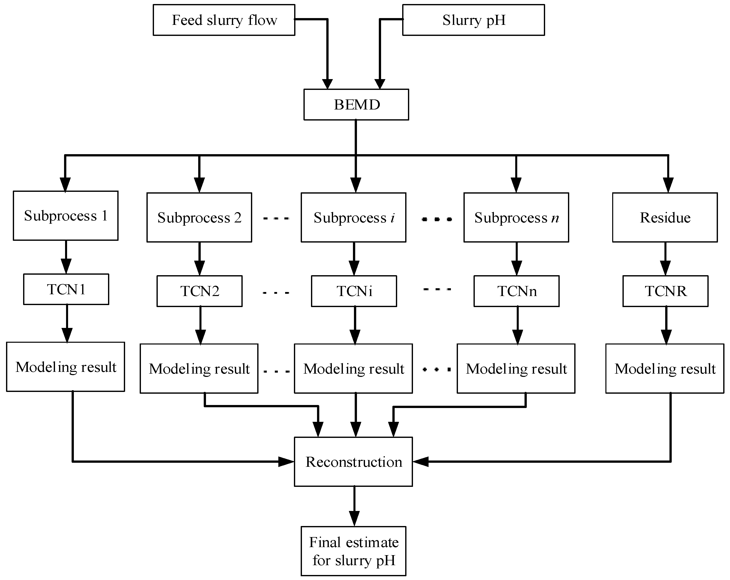
As stated earlier, properties like non-stationary/nonlinearity/long-term dependencies make the modeling of IFGD a truly formidable problem. It is known that the desired modeling performance cannot be achieved by employing traditional modeling methods mentioned above. To overcome this limitation, the BEMD-TCN approach, that hybridizes BEMD and TCN, is proposed to identify the IFGD process. The method mainly involves four steps.
Step 1: Collect measurements of limestone slurry flow and slurry pH in the reaction tank from the Continuous Emission Monitoring System (CEMS), which corresponds to the input and output signal of the IFGD process.
Step 2: A decomposition based on BEMD is conducted with respect to both input and output of the IFGD process; the resulting subprocess that consists of IMF pairs has a less complicated frequency component, and hence are comparatively easy to identify.
Step 3: According to the decomposed result, develop a well-structured TCN model for each subprocess and obtain the identification result.
Step 4: Sum up the identification result for each subprocess, and generate the final identification result for the IFGD process of interest.
Figure 2 schematically shows our approach.

3.1. Multivariate Empirical Mode Decomposition

EMD, as a data-driven and adaptive signal decomposition technique, is well suited to handle non-linear and non-stationary timeseries, with which a number of oscillatory modes (i.e., IMFs) are decomposed [21]. Comparing with the original system response, the degree of non-stationarity is reduced greatly in such oscillatory modes, hence, they are comparatively easy to identify. In this sense, EMD can be regarded as a tool for feature extraction before the process modeling, and the IFGD process modeling problem reduces to identifying each extracted subprocess. The process decomposition puts forward higher requirements for EMD, since both input and output signals are required for processing. The BEMD, which has the ability to handle cross-channel property in multivariate data, is chosen to decompose the multivariate signal that is made up of the process input and output.
Assuming that the reader is sufficiently familiar with the univariable EMD algorithm, its discussions may be found in [22]. In univariable EMD, the upper (lower) envelope is acquired by interpolating between all maxima (minima), then two envelopes are averaged to obtain the local mean. Since the local maxima (minima) cannot be defined in a direct way to overcome this problem, the BEMD algorithm proposed in [23] is introduced. In [23], the multivariate input signal is projected along different directions, then envelopes can be calculated according to the projected signal, and the local mean is approximated by averaging all directional envelopes in a multidimensional space. As the uniformity of direction vectors plays a significant role in approximation accuracy, it is central to choosing a suitable direction vector set. Considering a direction vector in n-dimensional space corresponds to a point on a unit (n − 1) sphere, to ensure the uniformity of direction vectors, a uniform sampling scheme should be adopted. In this work, low-discrepancy sampling approach suggested in [24] is adopted, by which more uniformly distributed points can be obtained. A multivariate IMF should ensure that the mean of the envelope must be equal to zero all the time; the difference with the univariate case is that the equality of extrema and zero crossings is not required [25]. Denoting the n-variate signal by  { v ( t ) } t = 1 T = { v 1 ( t ) , v 2 ( t ) , , v n ( t ) } , and  x θ k = { x 1 k , x 2 k , , x n k }  represents a direction vector which is characterized by angle  θ k = { θ 1 k , θ 2 k , , θ n 1 k }  on an (n − 1) unit sphere. Then, the multivariate EMD can be formulated as,
v ( t ) = i = 1 n f i ( t ) + R n ( t )
where,  f i ( t ) : n  denotes a decomposed IMF, and Rn(t) is the residue signal. The EMD algorithm for an n-variate timeseries is given below (see Algorithm 1).
Algorithm 1 Multivariate unidimensional EMD
  • Sample K points on a (n − 1) unit sphere using the low-discrepancy sampling approach.
  • For an input signal  { v ( t ) } t = 1 T , given a direction vector  x θ k , calculate the corresponding projected signal  { p θ k ( t ) } t = 1 T . Then, for K directions, the projection signal set  { p θ k ( t ) } k = 1 K  (t = 1, 2,…,T) can be obtained.
  • Search for time instants  { t θ k }  where maxima of projected signal  { p θ k ( t ) } k = 1 K  is achieved.
  • Interpolate  [ t i θ k , v ( t θ k ) ]  such that multivariate direction envelope curves  { e θ k ( t ) } k = 1 K  are obtained.
  • Calculate the mean  m ( t )  based upon K direction vectors as,
    m ( t ) = 1 K k = 1 K e θ k ( t )
  • The ‘detail’  d ( t )   is   extracted   as   d ( t ) = v ( t ) m ( t ) . If d(t) is an IMF, then set f(t) = d(t) and replace v(t) with the residue R(t) = v(t) − f(t). Otherwise, use d(t) in place of v(t) and repeat step 2–5.
  • Repeat steps 2–6 until all IMFs are extracted.
In our work, the flow of limestone slurry and slurry pH constitute the bivariate IMF. With the BEMD approach, processes are decomposed into multiple subprocesses that are defined by bivariate IMFs, then the IFGD modeling problem reduces to identify each SISO subprocess and aggregate them together. As can be seen, the originally challenging modeling problem has partitioned into multiple less complicated subproblems, and each of which is addressed separately. Despite the modeling complexity being significantly lowered, modeling IMFs is still by no means an easy task, and the principal difficulty is capturing the long-term dependencies between time steps. To accurately identify each IMF, TCN is chosen as the identification model and will be elucidated in greater detail below.

3.2. Temporal Convolutional Network for IFGD Process Identification

Convolution neural networks (CNNs) were first introduced to deal with problems in the computer vision field. More recently, in [26], a kind of CNN known as TCN was specially designed to deal with timeseries data. It was shown that TCNs outperform recurrent networks in terms of processing speed of timeseries with long-term dependencies, which is due to the parallel computation property of convolution. With most of the proposals over the year, TCNs is established as a timeseries model and used for forecasting purposes (see, e.g., [27,28]). Here, TCNs are introduced to identify an IFGD process, and the structure of TCNs used in our work is first described. In TCNs, 1D causal convolution rather than standard convolution is employed, which suggests the output of convolution operation at time t is solely on the basis past values. To model the IFGD process with long-term dependencies, it is of critical importance to expand the scope of local receptive field. However, for a standard causal convolution, there are two ways of expanding the coverage of model input, namely increasing the depth of layer or kernel size. Evidently, both approaches would impose a heavy computational burden for the network training. A simpler alternative is to introduce dilation convolution; let the input and output of an SISO process be denoted as u and y, respectively, then the output of a dilated convolution layer (denoted by ot) is written as,
o t = i = 0 k 1 a i y t d i + i = 0 k 1 b i u t d i
with d being the dilation factor, k being the size of filter and  a i / b i ( i = 0 , 1 , , k 1 ) being the kernel weight. An illustrative comparison among conventional convolution, causal convolution and dilated causal convolution is presented in Figure 3 below, wherein the layer number corresponding to three types of convolution operations remains the same, yet values of relevant hyperparameters are slightly different.
As shown above, with the same kernel size, the receptive field of causal CNN and dilated causal CNN are three and five, respectively. This implies that the introduction of dilation operation is an effective way to expand the receptive field, and d always increases exponentially with the depth of network. For causality-related CNN structures, the length of each output in hidden layer is made to be identical using zero padding. Another way to increase the receptive field is to deepen TCNs, however, this brings problems related to training deep neural network. Fortunately, the residual learning framework, proposed in [29], is effective in handling such problems, and the central idea of residual structure is to add the input of a layer directly to some layer output, which in the TCNs process modeling context can be formulated as
Y T = γ ( X T , W r ) + W s X T
where, the input multivariate signal  X T { x 1 T , , x n T }  and the component  x i T ( i = 1 , 2 , , n ) is one channel in  X T Y T  denotes a signal of appropriate dimension,  γ ( )  is known as the residual function which is of great flexibility and may consist of more than one layer, and Wr represents all parameters therein. Moreover, the weight matrix  W s  is introduced in the shortcut connection to keep the dimension of  γ ( )  consistent with that of shortcut’s output. Overall, the TCN model used in our work is established by cascading several residue blocks, which takes the form of (6) and  γ ( )  is realized by dilated causal convolution layer followed by a weight normalization layer, a ReLU nonlinearity and a dropout layer. The overall structure of the TCN model used in our IFGD modeling problem is presented in Figure 4.
It should be highlighted in Figure 4 that a unidimensional kernel instead of a two-dimensional one is used to convolve the multivariate input signal, which is marked in a yellow shaded area in the input tensor. The commonly used two-dimensional kernel acts on two-dimensional samples, say images, and the kernel moves along two directions (i.e., the height and width dimension). As for unidimensional kernel used here, it moves only along the time dimension such that information in time sequences can be extracted. In addition, only the input tensor for Residue Block 1 has two channels, while the input signal for other blocks is unichannel. In this case, the linear projection is a convolution kernel of size 2 × 1, while for other residue blocks can either be fixed to an identity matrix or just removed.
In what follows, the feasibility of using TCN for process modeling is illustrated from the system theory perspective. We shall use notations introduced in (2) and attempt to establish a link between the real process and TCN model. Irrespective of the residue architecture, the TCN model presented above can be mathematically expressed as follows.
y ^ ( k + 1 ) = φ ( N ) ( O N 1 ( k ) )
o ( n ) ( k ) = φ ( n ) ( O n 1 ( k ) ) , n = 1 , 2 , , N 1
o ( 0 ) ( k ) = x ( k ) = [ u ( k ) , y ( k ) ]
where, x(k) denotes input vector for the model,  k +  is the time instant, and  u ( k ) , y ( k )  denotes the system input and output, respectively.  φ ( )  is the sigmoidal activation function and  O n 1 ( k )  is defined as,
O n 1 ( k ) = [ o n 1 ( k ) , o n 1 ( k d ) , , o n 1 ( k ( i 1 ) d ) ]
where n is the number of layers and N is a positive constant. For mathematical convenience, both biases and kernel weights in (8) and (9) are omitted.  i , d +  denotes the kernel size and dilation factor, respectively. In comparison with the real process in form of (3), it is found that a complete TCN model can be regarded as the cascade connections of a finite number of models that in a simplified form of (3). In this sense, given a complicated dynamic process with long-term dependencies, from a theoretical point of view it can be well-approximated by increasing the depth or receptive field of a TCN model. In the following section, the performance of proposed BEMD-TCN model will be evaluated in an IFGD context.

4. Case Study and Discussion

4.1. Basic Information for the IFGD Process

To evaluate the identification performance of the developed approach, the mean absolute percentage error (MAPE) and root mean squared error (RMSE) are employed; they are defined as,
MAPE ( t ) = 1 N i = 1 N y ( t ) y ^ ( t ) y ( t )
RMSE ( t ) = 1 N i = 1 N ( y ( t ) y ^ ( t ) ) T ( y ( t ) y ^ ( t ) )
where, N is the total number of observations, and  y ( t )  and  y ^ ( t )  are, respectively, predicted and real process response. As for the experimental setup, all simulations are implemented on a PC computer with a NVIDIA Quadro P620 GPU, a 2.60 GHz Intel i7-10750 processor and 32 GB of memory.
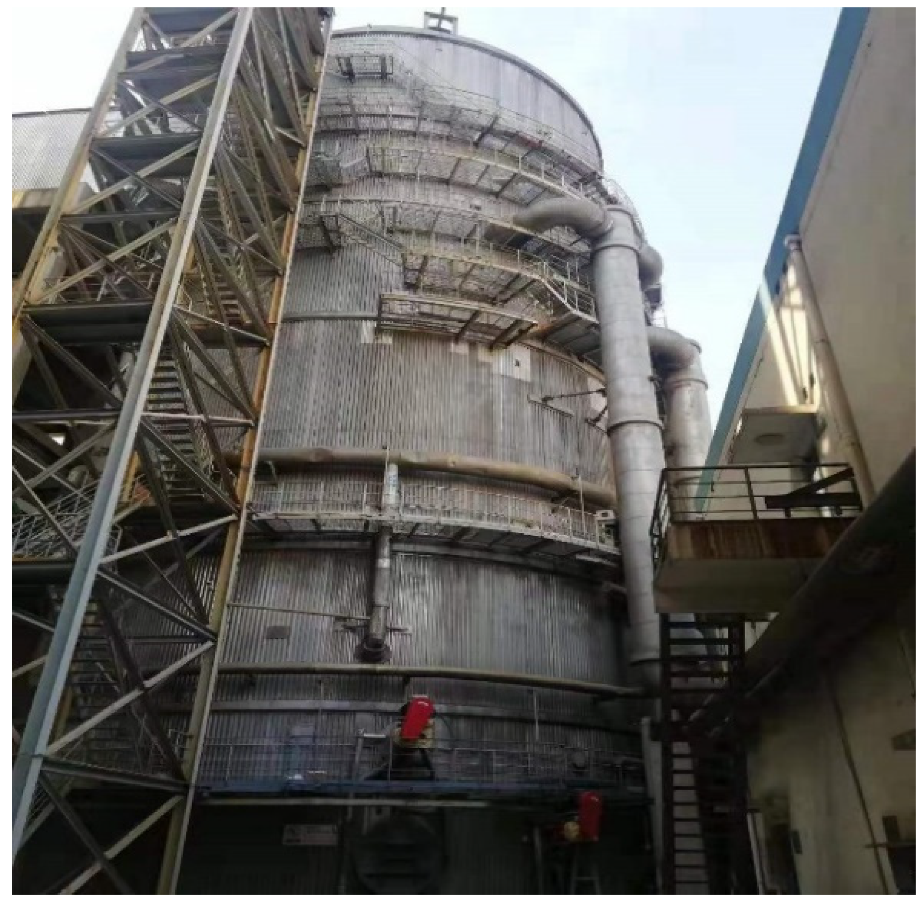
In our case study, we focus on the desulfurization system (see Figure 5) at a coal-fired power station with a 600 MW unit in China, and different modeling approaches are tested based upon collected historical running data. Since variations in electric power loads may necessitate changes in boiler load, the boiler loads and thus the operation mode of the IFGD process in various seasons differs significantly. Furthermore, slight fluctuations of daily boiler load are known to exist. The dataset consists of four parts, and each part encompasses a weekly observed data in a season; they are from 10 March 2021 to 17 March 2021, May 2021 to 28 May 2021, August 2021 to 12 August 2021 and 18 November 2021 to 25 November 2021. All data were sampled every 10 min within a fixed time interval in a day. Every part in dataset is separated into three subsets for training (70%), testing (15%) and validation (15%). Among three subsets, the training set is used for model building; the validation set serves as the early stopping criterion as well as the reference dataset to choose the best combination of hyperparameters, while the testing set plays the role of evaluating the final identification performance of the established model. To better understand the IFGD process under study, Table 1 lists the key statistical characteristics of variable slurry pH and slurry flow for four seasons, and slash is utilized to distinguish between two variables, wherein the former corresponds to process input (limestone slurry flow) while the latter is the output (slurry pH).

4.2. Case Study

In this section, representative data-driven methods for IFGD modeling used in previous research works are compared with the proposed approach. The methods are BP network, which is typically used as a benchmark in the IFGD modeling field (e.g., [6,14]), Hammerstein model in [30] and RNN in [31]. As for the RNN model, the back propagation through time (BPTT) algorithm proposed in [32] is used as the training algorithm; the stochastic gradient descent is employed for the BP network and the TCN with mini-batch size setting as 16, and the learning rate starts from 0.1 and is divided by 10 when the error plateaus. Training terminates after 200 epochs or once there was no improvement on the validation set for over six consecutive epochs. We use grid search to determine a good combination of hyperparameters for BP network and RNN (with the searching scope for hidden layer number {1,2,3,4}, hidden units {5, 20}) over the validation set. The determination of the TCN structure is realized by adjusting the depth of the network n and kernel size k, such that the receptive field covers sufficient input information for identification. To prevent the randomness of result brought about by the initial parameters in network, for each structure we run 20 trials with different initial weights, and the best-preforming one on the validation set is chosen and presented below. Hammerstein is a non-linear identifier with a linear dynamic and static nonlinearity cascading together, and extended least square [33,34] can be used for parameter estimation. Based on the performance on the validation set, the final model structure for above models is summarized in Table 2. It is noteworthy to mention that dilation factor d, kernel size k, layer number i and residue block number n are several most important parameters in TCN. Among them, exponential dilation technique is employed to expand the receptive field through layers, and we have  d = 2 i  for ith layer in the network. By adjusting k, i and n it was ensured that TCN has enough receptive field that is required for our IFGD identification task, and the result is also included in Table 2 below.
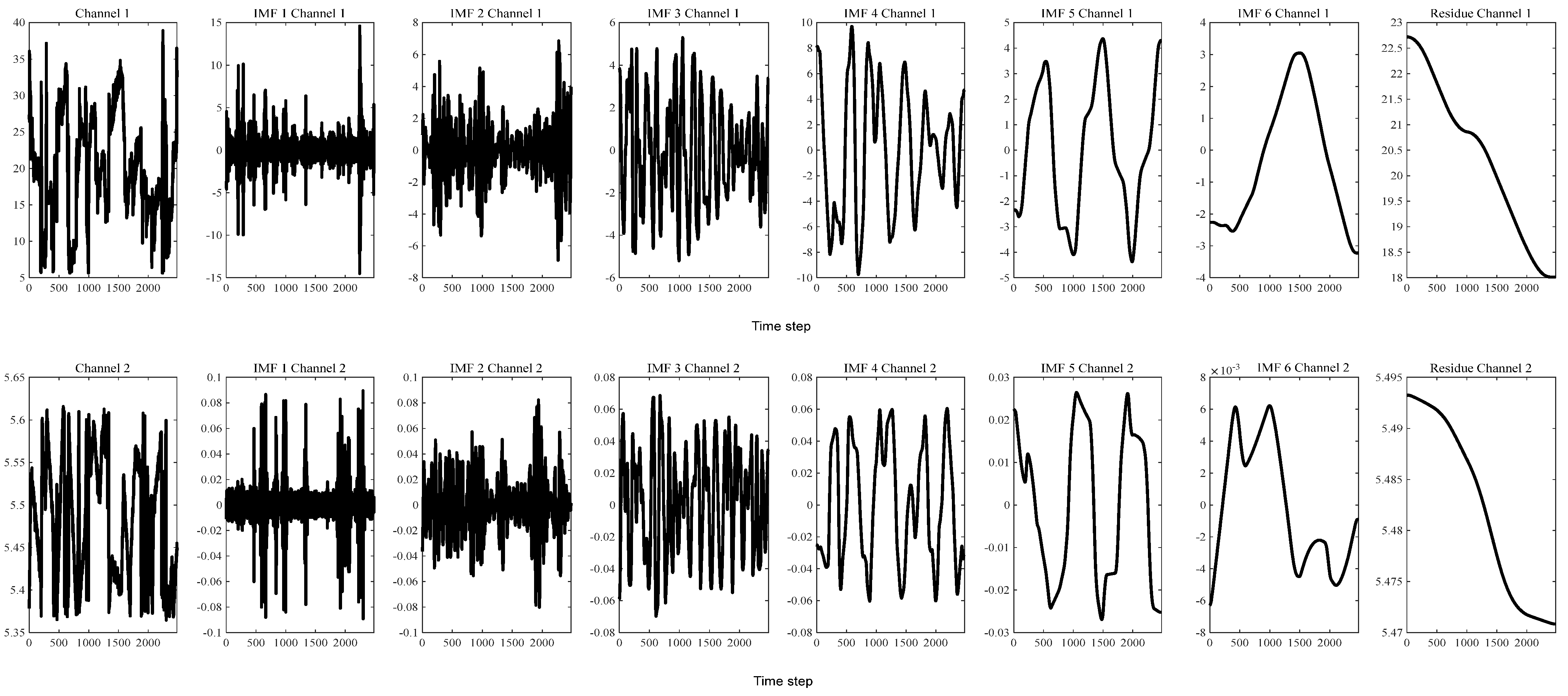
As for the BEMD-TCN approach, BEMD should be first performed to decompose the original IFGD process into several subprocesses, each of which is made up of corresponding IMF in two channels. In our case study, bivariate signal is made up of limestone feed flow and slurry pH and decomposed into six subprocesses (i.e., six groups of IMFs), due to space limitations and results for spring are presented in Figure 6 below.
Since the decomposed IMFs have less complex frequency components, lower amplitude and are relatively stationary, hence, resulting subprocesses are more readily to identify. Likewise, IMF pairs in other seasons can be decomposed by BEMD and are in turn used to constitute subprocesses.
Having decomposed process in each season into several parts, the next step is to use the TCN to identify each of them, and the final identification result is yielded by integrating them together. Keeping the same IMF number as that in spring, process in each season is partitioned into six IMFs and a residue. In BEMD, the signal in relatively high frequency is first extracted using the sifting process, and the residue can be considered as the trend from the point of view of timeseries analysis. The above fact illustrates that first decomposed subprocesses have more complicated dynamic behavior, which naturally calls for identifiers with greater structural complexity and hyperparameters are generally chosen by trial and error. With each decomposed subprocess at hand, corresponding TCN model is set up to identify it, and Table 3 summarizes the training performance for each subprocess with the use of suitably designed TCN models.
At this stage, for each season, a model set that consists of TCN models is established. Using (3) in conjunction with the model set, the final identification result on the test set can be easily obtained; corresponding results for four seasons are presented below. It can be clearly observed in Figure 7 that the proposed identification approach can fully capture complex non-linear effects in IFGD dynamics. The reason for this is twofold: on one hand, the originally highly complex process is decomposed into several subprocesses through BEMD, which have far fewer complicated frequency components and non-stationary properties, and are thus more simpler to identify; on the other hand, TCN has superior capability of representing nonlinearities and long-term dependencies while keeping the number of parameters in a low level. For a proper comparison, identification results of all approaches are listed in Table 4 below.
As shown in Table 4, identifiers of static nonlinearity type are found to perform poorly on the IFGD identification problem. Specifically, the BP network and the Hammerstein model performed similarly in all four seasons. In comparison, dynamic models can achieve better identifying performance. Among static and dynamic models, by choosing the best results for the four seasons separately, it is found that the score of MAPE (RMSE) is reduced from 0.0126 to 0.0041 (0.0801 to 0.0321) in spring, 0.0103 to 0.0039 (0.0761 to 0.0299) in summer, from 0.0109 to 0.0031 (0.0775 to 0.0236) in autumn, and from 0.0102 to 0.0025 (0.0758 to 0.0199) in winter. Overall, in all four seasons, the TCN model outperforms the other three models that appeared in the previous literature on IFGD identification in terms of MAPE and RMSE. Furthermore, with the proposed BEMD-TCN approach, the identification performance can be further improved, which has the minimum performance metrics, consequently, we can draw the conclusion that the BEMD-TCN is effective and can be well applied in the IFGD identification problem.

5. Conclusions

IFGD process identification problem has always been a challenging task in the industrial field. In our work BEMD-TCN approach is proposed to address this problem, where BEMD is used to decrease the non-stationary degree of the IFGD process, while TCN model is modified to model each subprocess. Comparative studies suggest that, among the models that appeared in the previous literature (i.e., RNN, BP network, Hammerstein model and TCN), our approach yields the best modeling performance in terms of MAPE and RMSE in all seasons. To be specific, the score of MAPE/RMSE reaches 0.00058/0.0059 in spring, 0.00089/0.0058 in summer, 0.00091/0.0063 in autumn, and 0.00062/0.0043 in winter. In this sense, the objective of accurate modeling industrial flue gas desulfurization process is achieved with the proposed approach. The proposed modeling approach is easily understandable while still assuring high modeling accuracy, and the authors believe that the method will find wide application in fault detection and intelligent control problems in the future.

Author Contributions

Conceptualization, X.L. and K.W.; methodology, X.L.; software, Q.L.; validation, X.L., Q.L. and K.W.; formal analysis, Q.L.; investigation, X.L.; resources, K.W.; data curation, X.L.; writing—original draft preparation, Q.L.; writing—review and editing, K.W.; visualization, X.L.; supervision, X.L.; project administration, X.L.; funding acquisition, X.L. All authors have read and agreed to the published version of the manuscript.

Funding

This research was funded by the National Natural Science Foundation of China, grant number 61873006; the Beijing Natural Science Foundation grant number 4212040.

Institutional Review Board Statement

Not applicable.

Informed Consent Statement

Not applicable.

Data Availability Statement

Not applicable.

Acknowledgments

The authors would like to thank the Editor-in-Chief for reading the manuscript and providing valuable comments. The authors would also like to thank the anonymous reviewers for their valuable comments and suggestions, which helped improve this paper greatly.

Conflicts of Interest

The authors declare no conflict of interest.

References

  1. Cui, L.; Liu, M.; Yuan, X.; Wang, Q.; Ma, Q.; Wang, P.; Hong, J.; Liu, H. Environmental and economic impact assessment of three sintering flue gas treatment technologies in the iron and steel industry. J. Clean. Prod. 2021, 311, 127703. [Google Scholar] [CrossRef]
  2. Dabadghao, V.; Biegler, L.T.; Bhattacharyya, D. Multiscale modeling and nonlinear model predictive control for flue gas desulfurization. Chem. Eng. Sci. 2022, 252, 117451. [Google Scholar] [CrossRef]
  3. Zhao, Z.; Fan, H.; Li, Q.; Liu, C.; Tan, C.; Chen, Z.; Yu, L.; Zheng, C.; Gao, X. Hybrid Modeling and Real-time Predictive Scheduling of Wet Flue Gas Desulfurization for Energy Saving and Life Extension. Energy Fuels 2023, 37, 5312–5322. [Google Scholar] [CrossRef]
  4. Brogren, C.; Karlsson, H.T. Modeling the absorption of SO2 in a spray scrubber using the penetration theory. Chem. Eng. Sci. 1997, 52, 3085–3099. [Google Scholar] [CrossRef]
  5. Zhao, Z.; Fan, H.; Li, Q.; Liu, C.; Chen, Z.; Li, L.; Zheng, C.; Gao, X. Hybrid modeling and operating optimization method of oxidation process of wet flue gas desulfurization (WFGD) system. Chem. Eng. Res. Des. 2022, 188, 406–416. [Google Scholar] [CrossRef]
  6. Guo, Y.; Xu, Z.; Zheng, C.; Shu, J.; Dong, H.; Zhang, Y.; Weng, W.; Gao, X. Modeling and optimization of wet flue gas desulfurization system based on a hybrid modeling method. J. Air Waste Manag. Assoc. 2019, 69, 565–575. [Google Scholar] [CrossRef]
  7. Krzywanski, J.; Nowak, W. Artificial intelligence treatment of SO2 emissions from CFBC in air and oxygen-enriched conditions. J. Energy Eng. 2016, 142, 04015017. [Google Scholar] [CrossRef]
  8. van Ewijk, S.; McDowall, W. Diffusion of flue gas desulfurization reveals barriers and opportunities for carbon capture and storage. Nat. Commun. 2020, 11, 4298–4308. [Google Scholar] [CrossRef]
  9. Li, X.; Han, J.; Liu, Y.; Dou, Z.; Zhang, T.A. Summary of research progress on industrial flue gas desulfurization technology. Sep. Purif. Technol. 2022, 281, 119849. [Google Scholar] [CrossRef]
  10. Liu, S.; Wu, Y.; Xu, Z.; Lu, S.; Li, X. Study on characteristics of organic components in condensable particulate matter before and after wet flue gas desulfurization system of coal-fired power plants. Chemosphere 2022, 294, 133668. [Google Scholar] [CrossRef] [PubMed]
  11. Grinišin, N.; Bešenić, T.; Kozarac, D.; Živić, M.; Wang, J.; Vujanović, M. Modelling of absorption process by seawater droplets for flue gas desulfurization application. Appl. Therm. Eng. 2022, 215, 118915. [Google Scholar] [CrossRef]
  12. Lancia, A.; Musmarra, D.; Pepe, F.; Volpicelli, G. SO2 absorption in a bubbling reactor using limestone suspensions. Chem. Eng. Sci. 1994, 49, 4523–4532. [Google Scholar] [CrossRef]
  13. Tseng, C.C.; Li, C.J. Numerical Investigations for the Two-Phase Flow Structures and Chemical Reactions within a Tray Flue Gas Desulfurization Tower by Porous Media Model. Appl. Sci. 2022, 12, 2276. [Google Scholar] [CrossRef]
  14. Uddin, G.M.; Arafat, S.M.; Ashraf, W.M.; Asim, M.; Bhutta, M.M.A.; Jatoi, H.U.K.; Niazi, S.G.; Jamil, A.; Farooq, M.; Ghufran, M.; et al. Artificial intelligence-based emission reduction strategy for limestone forced oxidation flue gas desulfurization system. J. Energy Resour. Technol. 2020, 142, 092103–092118. [Google Scholar] [CrossRef]
  15. Wen, J.; Yan, J.; Zhang, D.; Chi, Y.; Ni, M.; Cen, K. SO2 emission characteristics and BP neural networks prediction in MSW/coal co-fired fluidized beds. J. Therm. Sci. 2006, 15, 281–288. [Google Scholar] [CrossRef]
  16. Yu, H.; Gao, M.; Zhang, H.; Chen, Y. Dynamic modeling for SO2-NOx emission concentration of circulating fluidized bed units based on quantum genetic algorithm-Extreme learning machine. J. Clean. Prod. 2021, 324, 129170. [Google Scholar] [CrossRef]
  17. Cai, L.; Xu, Z.; Wang, X.; Bai, H.; Han, L.; Zhou, Y. Numerical simulation and optimization of semi-dry flue gas desulfurization in a CFB based on the two-film theory using response surface methodology. Powder Technol. 2022, 401, 117268. [Google Scholar] [CrossRef]
  18. Kang, Q.; Yuan, Y. Diagnosis and Traceability Analysis of Slurry Foaming of Limestone-Gypsum Wet Flue-Gas Desulfurization (WFGD) System. Water Air Soil Pollut. 2023, 234, 108. [Google Scholar] [CrossRef]
  19. Liu, T.; Garcia, P.; Chen, Y.; Ren, X.; Albertos, P.; Sanz, R. New predictor and 2DOF control scheme for industrial processes with long time delay. IEEE Trans. Ind. Electron. 2017, 65, 4247–4256. [Google Scholar] [CrossRef]
  20. Duan, S.; Zhao, C.; Wu, M. Multiscale partial symbolic transfer entropy for time-delay root cause diagnosis in nonstationary industrial processes. IEEE Trans. Ind. Electron. 2022, 70, 2015–2025. [Google Scholar] [CrossRef]
  21. Zare, M.; Nouri, N.M. A novel hybrid feature extraction approach of marine vessel signal via improved empirical mode decomposition and measuring complexity. Ocean. Eng. 2023, 271, 113727. [Google Scholar] [CrossRef]
  22. Kopsinis, Y.; McLaughlin, S. Development of EMD-based denoising methods inspired by wavelet thresholding. IEEE Trans. Signal Process. 2009, 57, 1351–1362. [Google Scholar] [CrossRef]
  23. Rehman, N.; Mandic, D.P. Multivariate empirical mode decomposition. Proc. R. Soc. A Math. Phys. Eng. Sci. 2010, 466, 1291–1302. [Google Scholar] [CrossRef]
  24. Dai, H.; Wang, W. Application of low-discrepancy sampling method in structural reliability analysis. Struct. Saf. 2009, 31, 55–64. [Google Scholar] [CrossRef]
  25. Mandic, D.P.; Goh, V.S.L. Complex Valued Nonlinear Adaptive Filters: Noncircularity, Widely Linear and Neural Models; John Wiley & Sons: Hoboken, NJ, USA, 2009. [Google Scholar]
  26. Bai, S.; Kolter, J.Z.; Koltun, V. An empirical evaluation of generic convolutional and recurrent networks for sequence modeling. arXiv 2018, arXiv:1803.01271. [Google Scholar]
  27. Sen, R.; Yu, H.F.; Dhillon, I.S. Think globally, act locally: A deep neural network approach to high-dimensional time series forecasting. Adv. Neural Inf. Process. Syst. 2019, 32, 241–251. [Google Scholar]
  28. Wan, R.; Mei, S.; Wang, J.; Liu, M.; Yang, F. Multivariate temporal convolutional network: A deep neural networks approach for multivariate time series forecasting. Electronics 2019, 8, 876. [Google Scholar] [CrossRef] [Green Version]
  29. He, K.; Zhang, X.; Ren, S.; Sun, J. Deep residual learning for image recognition. In Proceedings of the IEEE Conference on Computer Vision and Pattern Recognition, Las Vegas, NV, USA, 27–30 June 2016; pp. 770–778. [Google Scholar]
  30. Li, X.; Dong, J.; Wang, K. Constrained nonlinear model predictive control of pH value in wet flue gas desulfurization process. Optim. Control. Appl. Methods 2023, 44, 1523–1539. [Google Scholar] [CrossRef]
  31. Wu, Y.; Shen, L.; Zhang, L. Study on nonlinear pH control strategy based on external recurrent neural network. Procedia Eng. 2011, 15, 866–871. [Google Scholar] [CrossRef] [Green Version]
  32. Werbos, P.J. Backpropagation through time: What it does and how to do it. Proc. IEEE 1990, 78, 1550–1560. [Google Scholar] [CrossRef] [Green Version]
  33. Zhong, Y.; Yu, C.; Wang, R.; Pei, T.; Lian, L. Adaptive Anti-noise Least-Squares Algorithm for Parameter Identification of Unmanned Marine Vehicles: Theory, Simulation, and Experiment. Int. J. Fuzzy Syst. 2023, 4, 369–381. [Google Scholar] [CrossRef]
  34. Hao, X.; Wang, S.; Fan, Y.; Xie, Y.; Fernandez, C. An improved forgetting factor recursive least square and unscented particle filtering algorithm for accurate lithium-ion battery state of charge estimation. J. Energy Storage 2023, 59, 106478. [Google Scholar] [CrossRef]
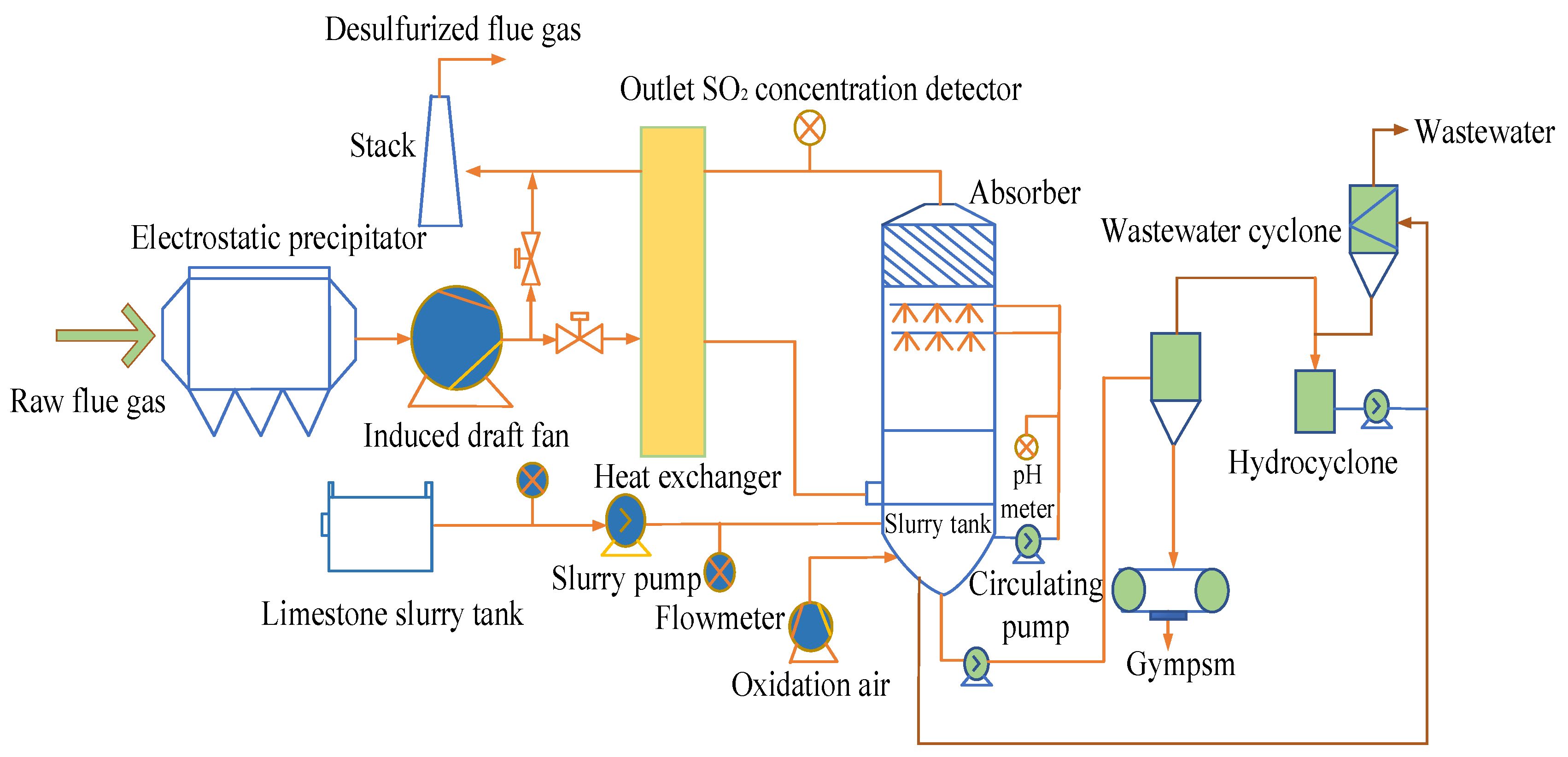
Figure 1. A schematic illustration of an IFGD process.
Applsci 13 07370 g001
Figure 2. Flowchart of BEMD-TCN approach.
Applsci 13 07370 g002
Figure 3. Comparison of different convolution structure. From left to right: conventional CNN with kernel size 3, causal CNN with kernel size 2 and dilated causal CNN with kernel size 2, dilation size 2.
Applsci 13 07370 g003
Figure 4. The overall architecture of TCN-based identification model for IFGD process.
Applsci 13 07370 g004
Figure 5. The photograph of desulfurization tower in the IFGD process.
Applsci 13 07370 g005
Figure 6. BEMD results in spring. (Upper) IMFs and residue for limestone feed flow. (Bottom) IMFs and residue for slurry pH.
Applsci 13 07370 g006
Figure 7. Identification results for IFGD process using BEMD-TCN approach.
Applsci 13 07370 g007
Table 1. Statistical characteristics of measured slurry pH in four different seasons.
SeasonStatistical Index
MinimumMaximumMeanSD 1Median
Spring5.504/5.36240.35/5.61318.84/5.4915.62/0.067518.84/5.499
Summer5.635/5.56337.14/5.82320.61/5.6817.041/0.058220.54/5.672
Autumn5.007/5.44650.53/5.69915.53/5.6325.323/0.043716.92/5.641
Winter5.43/5.52638.22/5.77819.11/5.6417.095/0.053419.17/5.623
1 SD denotes standard deviation.
Table 2. Optimal structure of candidate models.
SeasonModel Structure
BP NetworkRNNTCN (k-i-n)Hammerstein Model
Spring8-10-10-126-11-158-8-4 1.35 z 1 + 0.91 z 2 0.54 z 3 1 1.83 z 1 + 1.19 z 2 0.67 z 3 + 0.46 z 4
Summer12-15-88-164-6-3 0.49 z 1 0.41 z 2 1 2.21 z 1 + z 2 + 0.63 z 3 0.43 z 4
Autumn5-10-179-143-7-3 1 0.95 z 1 1 0.98 z 1 0.05 z 2 + 0.04 z 3
Winter10-16-96-12-108-16-4 0.72 + z 1 0.28 z 2 1 1.78 z 1 + 0.86 z 2 0.28 z 3 + 0.19 z 4
Note: (1) Sigmoid network is chosen as the nonlinearity in the above Hammerstein model, (2) For BP network and RNN network, the number of input and output units are omitted, e.g., 12-15-8 denotes a network that contains three hidden layers with 12, 15 and 8 units, respectively.
Table 3. Identification results for decomposed subprocesses in four different seasons.
SeasonMetricsIdentification Performance for BEMD Results
IMF1 1IMF2IMF3IMF4IMF5IMF6Residue
SpringMAPE0.99700.11300.03620.00670.00720.02680.00015
RMSE0.00230.000780.000240.000130.000860.000630.0011
SummerMAPE1.87310.43750.02010.00800.01520.18860.0016
RMSE0.00410.000660.000210.0000610.000190.00230.00013
AutumnMAPE2.00120.11800.01120.02200.01550.13020.0237
RMSE0.00470.00120.000740.000270.000230.000740.0052
WinterMAPE1.37120.43980.02110.01350.01480.24430.0076
RMSE0.00500.000760.000110.000320.000190.00300.00073
1 Subprocess is conventionally represented as IMF in the above table.
Table 4. Performance comparisons between different modeling methods.
SeasonMetricsApproaches
RNNBP NetworkHammersteinTCNBEMD-TCN
SpringMAPE0.00890.01280.01260.00410.00058
RMSE0.06450.08290.08010.03210.0059
SummerMAPE0.00610.02570.01030.00390.00089
RMSE0.04140.08510.07610.02990.0058
AutumnMAPE0.00510.02740.01090.00310.00091
RMSE0.03480.08600.07750.02360.0063
WinterMAPE0.00580.01250.01020.00250.00062
RMSE0.04040.08260.07580.01990.0043
Disclaimer/Publisher’s Note: The statements, opinions and data contained in all publications are solely those of the individual author(s) and contributor(s) and not of MDPI and/or the editor(s). MDPI and/or the editor(s) disclaim responsibility for any injury to people or property resulting from any ideas, methods, instructions or products referred to in the content.