Article

Predicting Critical Nodes in Temporal Networks by Dynamic Graph Convolutional Networks

1
Big Data Research Center, University of Electronic Science and Technology of China, Chengdu 611731, China
2
School of Information Engineering, Nanjing University of Finance and Economics, Nanjing 210023, China
3
Chengdu Union Big Data Technology Incorporation, Chengdu 610041, China
*
Author to whom correspondence should be addressed.
Appl. Sci. 2023, 13(12), 7272; https://doi.org/10.3390/app13127272
Submission received: 3 May 2023 / Revised: 11 June 2023 / Accepted: 17 June 2023 / Published: 18 June 2023
(This article belongs to the Special Issue Recent Advances in Big Data Analytics)

Abstract

:
Many real-world systems can be expressed in temporal networks with nodes playing different roles in structure and function, and edges representing the relationships between nodes. Identifying critical nodes can help us control the spread of public opinions or epidemics, predict leading figures in academia, conduct advertisements for various commodities and so on. However, it is rather difficult to identify critical nodes, because the network structure changes over time in temporal networks. In this paper, considering the sequence topological information of temporal networks, a novel and effective learning framework based on the combination of special graph convolutional and long short-term memory network (LSTM) is proposed to identify nodes with the best spreading ability. The special graph convolutional network can embed nodes in each sequential weighted snapshot and LSTM is used to predict the future importance of timing-embedded features. The effectiveness of the approach is evaluated by a weighted Susceptible-Infected-Recovered model. Experimental results on four real-world temporal networks demonstrate that the proposed method outperforms both traditional and deep learning benchmark methods in terms of the Kendall τ coefficient and top k hit rate.

1. Introduction

Nowadays, people’s lives are closely related to various complex networks, such as social [1], traffic [2] and email [3] networks. Network science is a vast and interdisciplinary research field and is a hot topic in many branches of sciences. Rich-club [4] shows that only a few critical nodes are needed to effectively affect and control the structure and function of the network. Therefore, to identify important nodes is thus significant, allowing us to find influential spreaders [5], control propagation of rumors [6] or epidemics, predict leading figures in academia, conduct advertisements for various commodities [7] and so on. For a variety of specific networks, key node mining can be targeted. In the power network, the protection of important circuit breakers and generating units can effectively prevent the large-scale blackout caused by successive failures [8]. In the application of a search engine, the search results can be sorted according to their matching and importance and returned to the user [9]. When an infectious disease occurs, the source of infection can be treated and isolated in a targeted way to effectively prevent the spread of the infectious agent [10].
In recent years, many critical nodes identification methods in static networks have been proposed [11,12,13]. Researchers have aimed to find critical nodes by some heuristic algorithms, such as degree centrality [14], betweenness centrality [15] and k-shell [5]. With the development of deep learning, many researchers are beginning to solve problems in their own fields with the help of deep learning. Representation learning-based  [16] methods embed a node as vectors or matrices, then design suitable learning frameworks to learn features of critical nodes, such as RCNN [17], InfGCN [18] and FINDER [19]. All these methods have good performances on various static networks.
However, many networks in the real world change over time. Temporal networks are not just an extension of static networks, which contain more in-depth and detailed information [20,21]. In temporal networks, the identification of critical nodes is not a trivial task. We can easily get the critical nodes in the current network by static methods, but we have no way of knowing whether the current critical nodes are still important in the future. Vital nodes can be identified in static networks, but can only be predicted in temporal networks. At present, there are two main research topics in this area: (1) methods based on structure and propagation dynamics [22]; (2) methods derived from dynamic graph neural networks (DGNNs) [23].
In order to exploit both structured data and temporal information, a new learning framework named the dynamic graph convolutional network (DGCN) is proposed. DGCN converts the problem of finding critical nodes in temporal networks to regression in deep learning. Our approach is based on the special graph convolutional network (GCN) and long short-term memory network (LSTM) [24]. GCN is a type of GNN which has roots in the convolutional neural network (CNN) [25] and is usually used to extract all levels of graph representation and perform graph classification tasks. LSTM is a special type of neural network with a hidden layer that recurs over time and is often used to process sequence data such as stock data. By combining the structural features learned by the special graph convolutional network with the temporal features learned by LSTM, DGCN can predict the node which has might have a strong spreading ability in the future. The performance of DGCN is compared with node2vec [26], struc2vec [27], temporal dynamics-sensitive centrality (TDC) [28] and temporal k-shell (TK) [29], by a weighted SIR model [30] on four real-world temporal networks. Experimental results show that DGCN can effectively predict nodes with the best spreading ability, and significantly outperforms benchmark methods in terms of Kendall τ coefficient and top k hit rate. Moreover, the training time of DGCN is linearly related to the size of networks and can be used for large networks.
The main contributions and novelties of this study are summarized as follows:
  • Convert the problem of finding critical nodes in temporal networks to regression in deep learning.
  • A novel and effective learning framework based on the combination of special GCNs and RNNs is proposed to identify nodes with the best spreading ability.
  • The proposed method is superior to both classical and state-of-the-art methods when applied to four real-world temporal networks.
  • It takes linear time complexity to deal with large networks with thousands of nodes and edges in a short time.
The remaining sections of the paper are as follows. Section 2 is a discussion of related works. Section 3 is the background for temporal networks, RNN and GCN. Section 4 is the detailed description of the proposed method. Section 5 is experimental results with analysis and discussion. Finally, conclusions are drawn in Section 6.

2. Related Works

To deal with the problems of identifying critical nodes in temporal networks, many methods based on structure and propagation dynamics have been proposed, and an intuitive idea is to extend methods in static networks such as degree, closeness and betweenness centrality to temporal networks. By this idea, Kim et al. [31] proposed the time-ordered graph, embedding dynamic networks into directed and static networks. This enables us to extend network properties in a very natural way to the dynamic case. Huang et al. [28] proposed the temporal version of dynamic-sensitive centrality, which extends dynamic-sensitive centrality [32] to temporal networks by the Markov chain for the epidemic model, and the numerical simulation shows that the new centrality performs much better than some topological structural centralities. By coupling centrality matrices in each snapshot into a supracentrality matrix, Taylor et al. [33] proposed an extension framework for static centrality measures such as eigenvector-based centrality and introduced the concepts of marginal and conditional centralities, which facilitate the study of centrality trajectories over time. Huang et al. [34] defined a supra-evolution matrix to describe the structure of temporal networks. with using of the time series analysis, the relationships between different time layers can be learned automatically. Based on the special form of the supra-evolution matrix, the eigenvector centrality calculating problem is turned into the calculation of eigenvectors of several low-dimensional matrices through iteration, which effectively reduces the computational complexity. This type of method can find critical nodes in the current temporal network but can not predict the importance of nodes in the future. To find the most influential nodes, Chandran et al. proposed a method [35] which measures the impact of each node by the triangle property based on 2-hop neighbors. Jiang et al. proposed an attenuation-based supra-adjacency matrix (ASAM) [36] to model temporal networks and evaluated the importance of nodes in temporal network by calculating the eigenvector centrality of the nodes in each time layer. Bi et al. proposed a temporal gravity model [37] which treats basic node properties as the mass and temporal characteristics as the distance to identify important nodes in temporal networks.
In recent years, graph neural networks (GNNs) have become research hotspots and have been used to solve graph-related problems, such as graph [38,39] and node [26,27] classification. Among them, DGNN [40] has recently prevailed deep learning models used to deal with temporal graphs, which often make use of a graph neural network (GNN) [41] and recurrent neural network (RNN) [42]. GCRN-M [43] stacks a spectral GCN [44] and a standard LSTM to predict structured sequences of data. DyGGNN [45] uses a gated graph neural network (GGNN) [46] combined with a standard LSTM to learn the evolution of dynamic graphs. Chen et al. [47] present GC-LSTM, which performs a spectral GCN on the hidden layer of the standard LSTM for dynamic link prediction. At present, DGNNs are mainly aimed at learning representations of entire dynamic graphs, such as DGNN, GCRN-M and DyGGN. The learning framework specific to nodes in temporal networks is still lacking. A novel framework which defined a GNN based model that learns the implicit features of nodes on a representative set is proposed by Munikoti et al. [48], but this representation does not apply to temporal networks. The above works cannot embed the nodes of temporal networks well. In this paper, a novel and effective learning framework DGCN is proposed to embed nodes in temporal networks.

3. Background

In this section, we provide a brief introduction to the required background in temporal networks and graph neural networks.

3.1. Temporal Networks

Temporal networks can be divided into continuous-time representation and discrete-time representation networks.There is a big difference between the discrete-time and continuous-time temporal networks in modeling methods, and the method of identifying key nodes is not universal. In this paper, we only consider the discrete-time temporal networks. A discrete-time temporal network T G with time range [ 0 , T ] can be defined as a set of ordered static networks (snapshots). That is, T G = { G 1 , G 2 , , G L } where L = T / δ represents the number of snapshots, which is determined by the time span T and the time interval δ of each snapshot. G t = { V t , E t } represents the spanning subgraph G t which consists of nodes V t and edges E t appearing in [ δ · ( t 1 ) , δ · t ] .

3.2. Recurrent Neural Network

A recurrent neural network (RNN) [49] is a special type of neural networks with a hidden layer that recur over time and often used to process sequence data such as stock data. Unlike other neural networks, RNN implement the structure which retains a certain memory of past information. Among of all RNNs, Bidirectional RNNs (Bi-RNNs) [50] and long short-term memory networks (LSTM) [51] are widely used. The standard RNN is based on a simple repeating cell. LSTM extends the repeating cell by combining four interacting units.

3.3. Graph Neural Network

A graph neural network (GNN) [52] combines graph data with neural networks, and performs calculations on graph data. A graph convolutional network (GCN) is usually used to extract all levels of graph representation and perform graph classification tasks. A GCN follows the framework of exchanging information with neighbors and the key issue is to aggregate the node features from its neighborhood.

4. Method

4.1. Problem Definition

The problem of predicting important nodes can be converted to a regression problem in deep learning. Suppose temporal network T G = { G 1 , G 2 , , G L } , a function f needs to learn:
S c o r e l = f ( G l s , G l s + 1 , , G l 1 ) , l [ s + 1 , L + 1 ]
where S c o r e l is the predicted score for nodes which have appeared before time l in G l , and s is the number of input snapshots. We know that GCN can effectively deal with static graph data and RNN is good at handling sequence data.
The research is divided into two stages: (1) if the importance of a node in each snapshot can be learned through GCN, then we can get a sequence containing the importance of the node in each snapshot; (2) the importance of the node in the future can be predicted by using the sequence as the input of RNN. Combining GCN and RNN, a new learning framework named dynamic graph convolutional network (DGCN) is proposed to predict critical nodes in temporal networks.

4.2. Dynamic Graph Convolutional Network

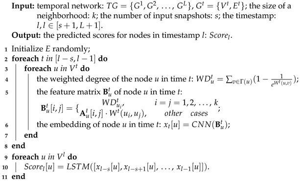
In this subsection, a framework of DGCN for learning representations from arbitrary temporal networks is proposed. The process of DGCN is shown in Figure 1. In DGCN, we replace a standard snapshot with a weighted snapshot to describe the temporal network in a finer granularity and the weighted degree is used to distinguish neighbors of the same hop in determining the node’s neighborhood. The step-weighted snapshot to step the CNN layer can be regarded as a special GCN which implicitly outputs the importance of nodes at time t, essentially, a process of node embedding.
The overall DGCN is shown in Algorithm 1. The input is a temporal network T G and the output is the influence of nodes in timestamp l. DGCN first calculates the embedding of all nodes at each snapshot and then uses LSTM to predict the importance of nodes in the future. The details of each step are explained below:
Algorithm 1: The flow of DGCN.
Applsci 13 07272 i001
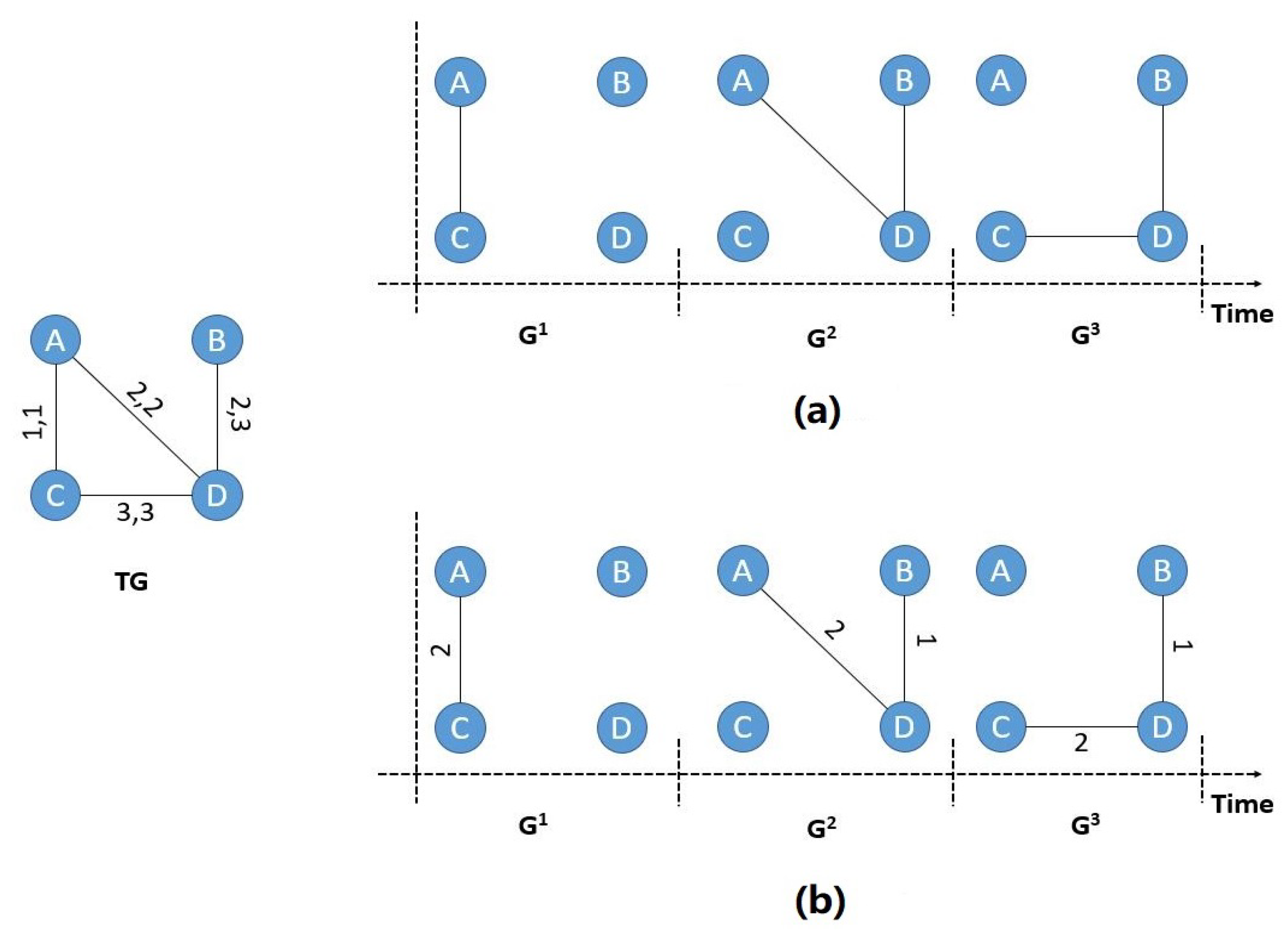
Weighted Snapshots: Divide the temporal network T G into L snapshots according to the time interval δ , T G = { G 1 , G 2 , , G L } where L = T / δ . As shown in Figure 2, in the standard snapshot G t = { V t , E t } , E t contains all edges that appear in the time interval [ δ · ( t 1 ) , δ · t ] . This processing method is coarse-grained, because there may be multiple contacts between nodes in a time interval, but it is only retained once in the snapshot. In order to accurately describe the relationship between a node and its neighbors in a temporal network, weighted snapshots are proposed. In a weighted snapshot G t = { V t , E t , W t } , W t records the number of occurrences of each edge in the time interval [ δ · ( t 1 ) , δ · t ] . W t ( u , v ) = w only if e u , v appears w times in [ δ · ( t 1 ) , δ · t ] . Compared with the standard snapshot, the number of node interactions in the time interval is considered in a fine-grained manner. In addition, in order to ensure data consistency, each snapshot contains all nodes.
Node Neighborhood: Suppose the size of a neighborhood is k, that is, we need to find k 1 neighbors for each node and number neighbors according to order. The strategy for selecting neighbors from a snapshot is as follows; the first priority is the distance between the node and the neighbor. In the same distance, prioritize neighbors with high weighted degree. The weighted degree takes into account the weight of edges in weighted snapshots, and the weighted degree of the node u in time t is defined as:
W D u t = v Γ ( u ) ( 1 1 e W t ( u , v ) ) .
After selecting enough neighbors, for each node, such as node u, generate the subnetwork G u t which contains node u and its k 1 neighbors from the snapshot G t . For example, in Figure 2b, suppose k = 3 , G A 2 contains node A, D and B; G D 3 contains node D, C and B.
Node Feature Matrix: For each subnetwork, such as G u t , A u t is the adjacency matrix of G u t and the feature matrix of node u is defined as:
B u t [ i , j ] = W D u i t , i = j = 1 , 2 , , k A u t [ i , j ] · W t ( u i , u j ) , o t h e r c a s e s
where u 1 , u 2 , . . . , u k are node u and its k 1 neighbors respectively. O u i t is the out degree of node u i in the snapshot G t . In addition, if G t is disconnected, we might not find enough neighbors for node u, and we need expand B u t with dummy node to have same shape matrices. For example, in Figure 2b, if k = 3 , G A 2 contains node A, D and B, A A 2 and B A 2 are shown as follow:
A A 2 = 0 1 0 1 0 1 0 1 0 , B A 2 = 1 2 0 2 2 1 0 1 1
If k = 5 , we need add 2 dummy nodes and B A 2 are shown as:
B A 2 = 1 2 0 0 0 2 2 1 0 0 0 1 1 0 0 0 0 0 0 0 0 0 0 0 0
CNN Layer: The CNN in this layer is the same as the CNN in R C N N [17]. Through the convolution processing of feature matrices, the importance of nodes can be implicitly expressed. There are two reasons why we use the same CNN to train nodes in different snapshots instead of training a separate CNNs for each snapshot: (1) Global training does not change the importance ranking of nodes in the same snapshot, and can effectively reduce training parameters. (2) By increasing the number of input snapshots s, a large number of training nodes can be quickly obtained.
LSTM Layer: A standard LSTM [51] is used in this layer, and the input element in time t is x t = C N N ( B u t ) . In addition, the input size is 1, hidden size is 64 and the number of recurrent layers is 2. Finally, a fully connected layer is used to output the predicted score for nodes.
Weighted SIR Model and Label: The influence of nodes over a period of time is usually measured by SIR spreading model. In this paper, we use weighted SIR model to measure the influence of nodes in discrete-time temporal networks. In the SIR model [30], each node has one of three states, i.e., susceptible, infected or recovered. In time interval [ δ · ( t 1 ) , δ · t ] , infected nodes will infect their susceptible neighbors with a probability β and recover with a probability μ . Particularly, in the weighted SIR model, the susceptible node u will be infected by the infected neighbor v with 1 ( 1 β ) W t ( v , u ) . N u t ( x ) is defined as the number of recovered and infected nodes after x intervals under weighted SIR model from the initial infected node u in snapshot G t . N u t ( x ) can be used to represent the importance of u in snapshot G t in this paper.
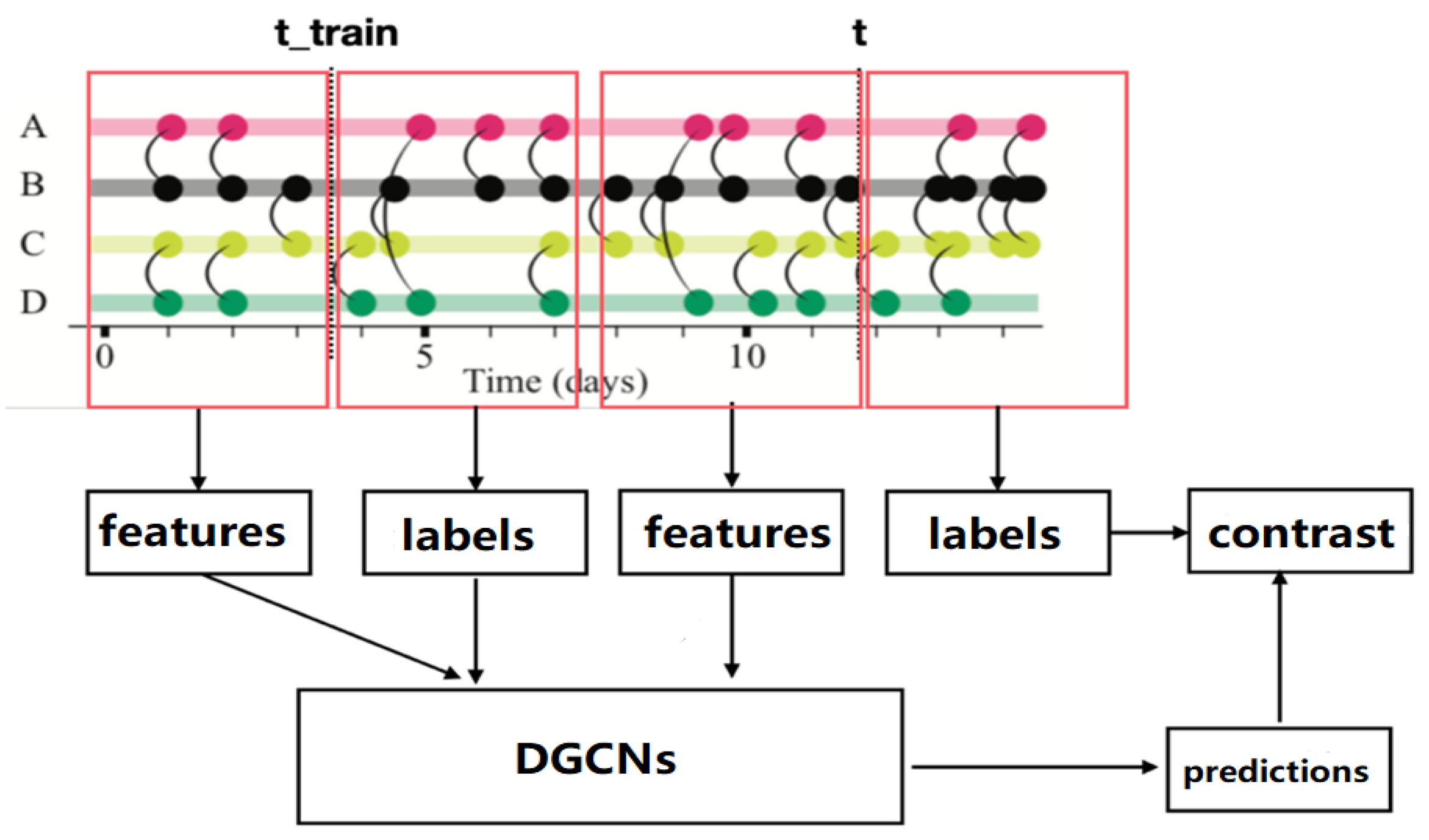
As shown in Figure 3, for a temporal network T G = { G 1 , G 2 , , G L } , the task is to predict the importance of nodes in snapshot G t ( t L 10 ) with training data being { G 1 , G 2 , , G t 1 } . Because ten snapshots are used to generate the label, { G t 11 s , , G t 11 } is used as the training set and N t 10 ( 10 ) as the label in the model, and the number of input snapshots s is also needed to determine by traversing L. The loss function is a squared loss function.

4.3. Complexity Analysis

Let the temporal network be T G = { G 1 , G 2 , , G L } , the size of the neighborhood be k ( k < < N ) and use s snapshots to train DGCN. For each snapshot and node, the time complexity of generating the feature matrix is O ( k 2 ) , the time complexity of CNN is O ( k 2 ) [17] and the time complexity of LSTM is O ( N ) . So the time complexity of DGCN is O ( s 2 · I · k 2 · N ) , where I is the number of training iterations. Actually, when all parameters are fixed, the complexity of DGCN is linearly related to the number of nodes in the temporal network.

5. Experiments

In this section, datasets, experimental settings and results achieved by DGCN are described in detail.

5.1. Datasets

Four real-world temporal networks are selected to evaluate the proposed method. Some basic properties of these networks are listed in Table 1.
  • Email [53]. The directed temporal network is generated by the mail data from a research institution in Europe.
  • Contact [54]. An undirected temporal network contains connections between users using mobile wireless devices. An edge is generated if two people are in contact.
  • DNC [55]. A directed temporal network of emails in the 2016 Democratic National Committee email leak.
  • UCI [56]. A directed temporal network contains sent messages between students at the University of California, Irvine.

5.2. Experimental Settings

In this paper, for each dataset, the training set is { G 31 s , G 31 s + 1 , , G 30 } , s [ 1 , 30 ] with label N 31 ( 10 ) (training infection rate β t = 0.05) and testing set is { G 41 s , G 41 s + 1 , , G 40 } with label N 41 ( 10 ) . That is, for DGCN and all benchmark methods, the snapshot G t ( t > 40 ) is unknown, only G t , t 40 can be used to predict the importance of nodes in G 41 . Finally, compare the prediction results with N 41 ( 10 ) to verify the performance of the methods. In addition, the GPU for all experiments is 1600 MHz with 8G memory. In the field of deep learning, GPU is often used to train models, and subsequent experiments are compared on the same GPU.

5.3. Benchmark Methods

In order to effectively evaluate the performance of DGCN, benchmark methods include two types; one is based on network structure and propagation dynamics, and the other is based on graph neural networks.
The temporal k-shell (TK) [29] is defined as
T K ( v ) = u Γ v t = 1 L m i n k s t ( v ) , k s t ( u )
where k s t ( v ) is the k-shell of node v and Γ v is the neighbors of node v in snapshot t.
Temporal dynamics-sensitive centrality (TDC) [28] is defined as
S = r = 0 L 1 β H * r A r + 1 X
H * t = α = t 1 [ β A α + ( 1 μ ) I ] , H * 0 = 1
where S i is the score of node i and X = ( 1 , 1 , , 1 ) T , μ and β are parameters of the SIR Model.
The core of DGCN is how to embed nodes in no-attribute graphs, and can be replaced by other well-known node-embedding methods, such as node2vec [26] and struc2vec [27]. In this paper, the replaced methods are called N2V-LSTM and S2V-LSTM. These two methods embed nodes of each snapshot and input them into LSTM.

5.4. Results

As we know, for the problem of predicting the importance of nodes in temporal networks, the closer the predicted ranking is to the real ranking (simulated value of the SIR Model), the better the performance of the method. Here, we use the kendall τ correlation coefficients [57] to measure the performance of all methods.
Firstly, we perform a sensitivity analysis of the number of input snapshots s on DGCN. In Figure 4, we show the impact of s on final kendall τ between the real ranking and predicted ranking with the infection rate β = 0.05 . From Figure 4, in the email network, the time interval is 168 h (a week), when s is less than 5, the performance of DGCN improves as s increases, and then it stays in a steady state. This means that the importance of a user in the next 10 weeks can be predicted only by using the data in the past 5 weeks and more data is not necessary for improving the performance. In the contact network, the time interval is 1 h, DGCN is almost unaffected by s while performing extremely well. This also means that only the data of the past 1 h are needed to predict the importance of the user in the next 10 h very accurately. In the DNC network, the time interval is 12 h; it can be seen that the performance of DGCN reaches its peak at s = 4 and then shows a downward trend. This indicates that the data of the past 48 h are sufficient to predict the importance of the user in the next 120 h. However, very old historical data will bring a lot of noise, which will seriously affect the performance of DGCN. Similar to the DNC network, in the UCI network, the time interval is 24 h (1 day), the performance of DGCN reaches its peak at s = 2 and then shows a downward trend. These results show that in different temporal networks, the historical data needed to predict the importance of nodes are not as much as possible. Very old data may even have a negative impact on the prediction results. So far, the optimal value of s for different networks can be selected by an exhaustive search.
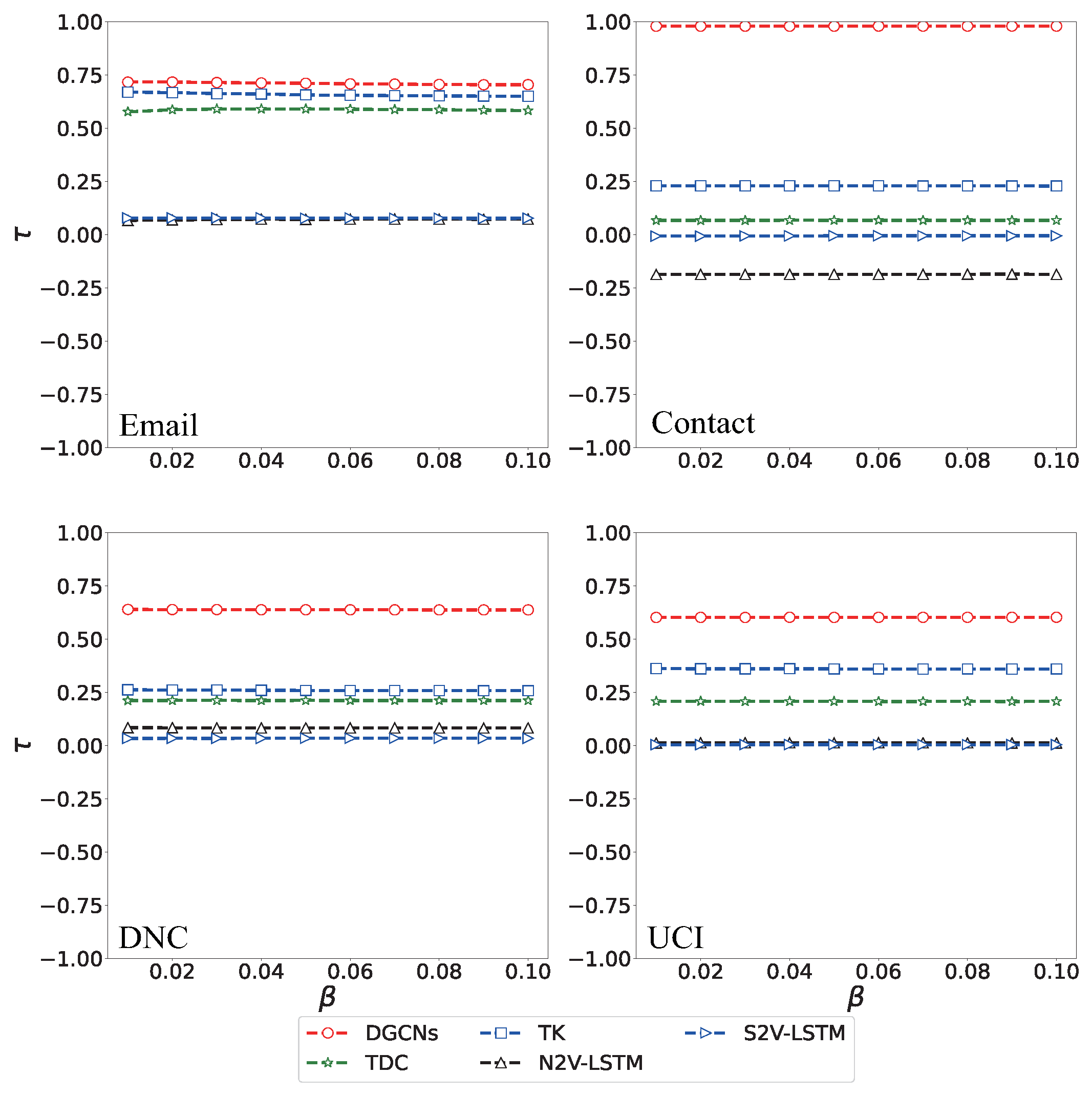
After determining s, from Figure 5, compared with other methods, no matter how the infection rate β changes, DGCN has the highest kendall τ correlation coefficients. This means that among all the methods, the ranking result of DGCN is the closest to the real ranking result. In addition, we can see that the performances of N2V-LSTM and S2V-LSTM are very poor in all networks, especially in the contact network. This shows that a simple combination of deep learning models cannot solve some professional problems in the field of complex networks. An effective and feasible learning framework needs to be designed with more knowledge in related fields. In DGCN, we not only consider the local characteristics of the nodes but also the multiple interactions of the nodes in the same snapshot. These features will significantly affect the information transmission ability of the nodes.
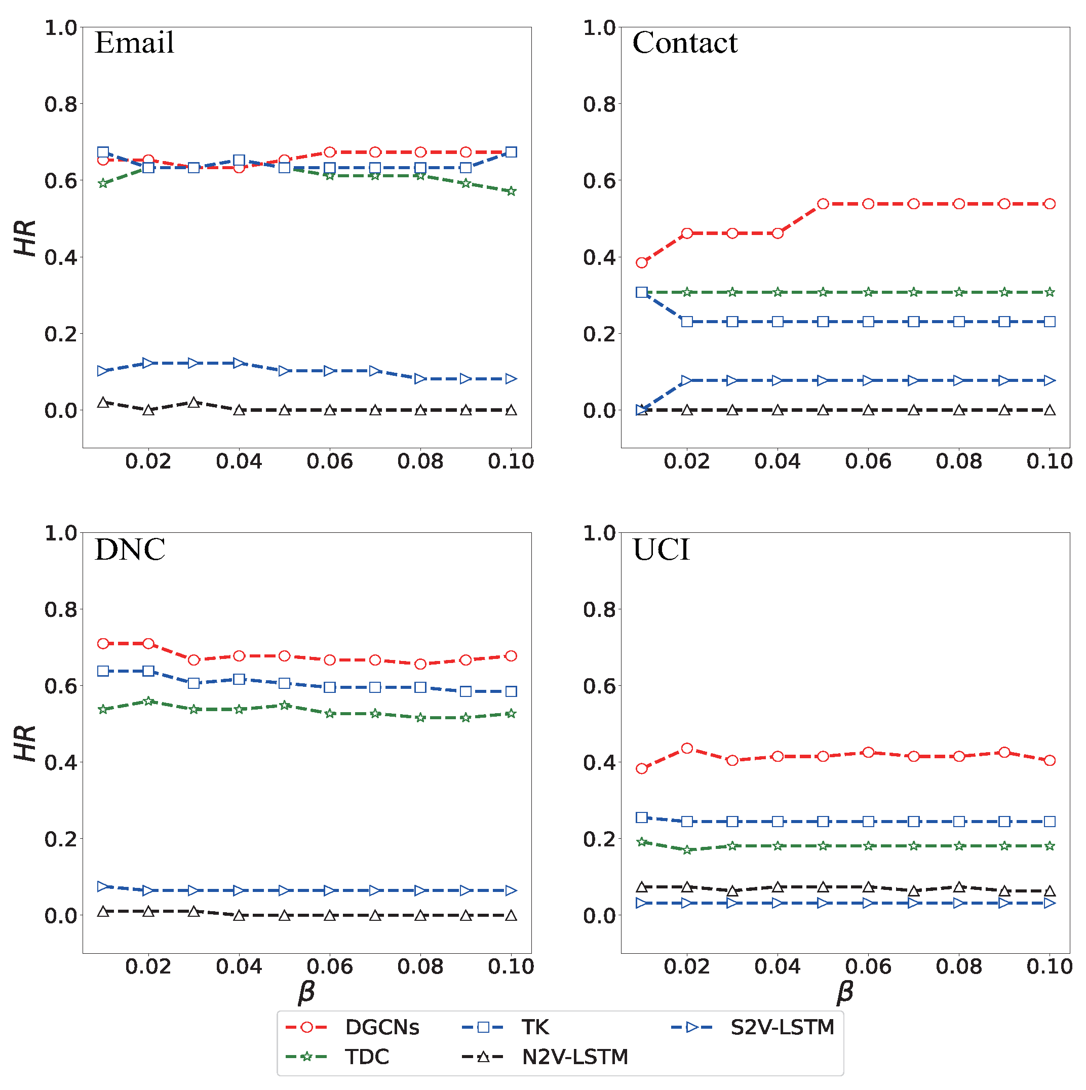
In real life, people usually care more about top k nodes than the ranking of nodes. So we compared the hit rate of top k nodes of all methods. For details, the top k hit rate can be defined as
H R = | P R | | R |
where P is the set of top k nodes in predicted ranking and R is the set of top k nodes in real ranking. Obviously, the best method should have the largest H R . From Figure 6, it can be seen that DGCN outperforms other methods in most cases under a different infection rate β . These results further prove the effectiveness of DGCN.
Finally, The time costs of the above five methods are compared. Table 2 shows the training time of DGCN on four temporal networks with different s. It can be seen that DGCN spends very little training time. Table 3 shows the time cost of ranking nodes by all methods. From Figure 6 and Table 3, although DGCN is not the fastest algorithm, it achieves the best results in an acceptable time and is scalable in linear time complexity.

6. Conclusions

In this work, we introduce a new learning framework, DGCN, which can predict the importance of nodes in temporal networks. The model consists of a special graph convolutional network and a long-short term memory network. We have assessed the performance of DGCN on four real-world networks against some benchmark methods. The results show that the ranking by DGCN is the closest to the real ranking (no matter how the infection rate β changes, DGCN has the highest kendall τ correlation coefficients) and has the highest top k hit rate. Furthermore, the training time of DGCN is linearly related to the number of nodes and can be used for large-scale networks. Like most current models, DGCN relies on snapshots, which are relatively crude temporal representations. Continuous time methods can often capture more in-depth and detailed information. Hence, how to extend DGCN to continuous-time temporal networks is one of the main tasks in the future, and another interesting extension of our work is critical edges prediction in temporal networks.

Author Contributions

Conceptualization, E.Y. and D.C.; methodology, E.Y.; validation, E.Y., Y.F. and J.Z.; formal analysis, E.Y., H.S. and D.C.; investigation, E.Y.; data curation, E.Y.; writing—original draft preparation, E.Y.; writing—review and editing, D.C., Y.F., J.Z. and H.S.; supervision, Y.F.; funding acquisition, D.C. and H.S. All authors have read and agreed to the published version of the manuscript.

Funding

This work is jointly supported by the National Natural Science Foundation of China under Grant Nos. 61673085 and 71901115, by the Science Strength Promotion Programme of UESTC under Grant No. Y03111023901014006, by the International Cooperation Programme of JiangSu Province under Grant No BZ2020008, by the Young Scholar Programme from NUFE under Grant No SHLXW19001 and by the National Key R&D Program of China under Grant No. 2017YFC1601005.

Institutional Review Board Statement

Not applicable.

Informed Consent Statement

Not applicable.

Data Availability Statement

The data presented in this study are available on request from the corresponding author. The data are not publicly available due to the original URL of the data can’t achieve now.

Conflicts of Interest

The authors declare no conflict of interest.

References

  1. Weng, J.; Lim, E.P.; Jiang, J.; He, Q. TwitterRank: Finding topic-sensitive influential twitterers. In Proceedings of the WSDM 2010-Proceedings of the 3rd ACM International Conference on Web Search and Data Mining, New York, NY, USA, 3–6 February 2010; pp. 261–270. [Google Scholar]
  2. Ghosh, S.; Banerjee, A.; Sharma, N.; Agarwal, S.; Ganguly, N.; Bhattacharya, S.; Mukherjee, A. Statistical analysis of the Indian Railway Network: A complex network approach. Acta Phys. Pol. B Proc. Suppl. 2011, 4, 123–137. [Google Scholar] [CrossRef]
  3. Guimerà, R.; Danon, L.; Díaz-Guilera, A.; Giralt, F.; Arenas, A. Self-similar community structure in a network of human interactions. Phys. Rev. E-Stat. Phys. Plasmas Fluids Relat. Interdiscip. Top. 2003, 68, 065103. [Google Scholar] [CrossRef] [Green Version]
  4. Colizza, V.; Flammini, A.; Serrano, M.A.; Vespignani, A. Detecting rich-club ordering in complex networks. Nat. Phys. 2006, 2, 110–115. [Google Scholar] [CrossRef] [Green Version]
  5. Gallos, L.; Havlin, S.; Kitsak, M.; Liljeros, F.; Makse, H.; Muchnik, L.; Stanley, H. Identification of influential spreaders in complex networks. Nat. Phys. 2010, 6, 888–893. [Google Scholar]
  6. Zhou, F.; Lü, L.; Mariani, M.S. Fast influencers in complex networks. Commun. Nonlinear Sci. Numer. Simul. 2019, 74, 69–83. [Google Scholar] [CrossRef] [Green Version]
  7. Zhang, T.; Li, P.; Yang, L.X.; Yang, X.; Tang, Y.Y.; Wu, Y. A discount strategy in word-of-mouth marketing. Commun. Nonlinear Sci. Numer. Simul. 2019, 74, 167–179. [Google Scholar] [CrossRef]
  8. Wang, S.; Lv, W.; Zhang, J.; Luan, S.; Chen, C.; Gu, X. Method of power network critical nodes identification and robustness enhancement based on a cooperative framework. Reliab. Eng. Syst. Saf. 2021, 207, 107313. [Google Scholar] [CrossRef]
  9. Joodaki, M.; Dowlatshahi, M.B.; Joodaki, N.Z. An ensemble feature selection algorithm based on PageRank centrality and fuzzy logic. Knowl.-Based Syst. 2021, 233, 107538. [Google Scholar] [CrossRef]
  10. Wei, X.; Zhao, J.; Liu, S.; Wang, Y. Identifying influential spreaders in complex networks for disease spread and control. Sci. Rep. 2022, 12, 5550. [Google Scholar] [CrossRef]
  11. Lü, L.; Chen, D.; Ren, X.L.; Zhang, Q.M.; Zhang, Y.C.; Zhou, T. Vital nodes identification in complex networks. Phys. Rep. 2016, 650, 1–63. [Google Scholar] [CrossRef] [Green Version]
  12. Guo, C.; Yang, L.; Chen, X.; Chen, D.; Gao, H.; Ma, J. Influential nodes identification in complex networks via information entropy. Entropy 2020, 22, 242. [Google Scholar] [CrossRef] [Green Version]
  13. Chen, D.B.; Sun, H.L.; Tang, Q.; Tian, S.Z.; Xie, M. Identifying influential spreaders in complex networks by propagation probability dynamics. Chaos 2019, 29, 030120. [Google Scholar] [CrossRef]
  14. Bonacich, P. Factoring and weighting approaches to status scores and clique identification. J. Math. Sociol. 1972, 2, 113–130. [Google Scholar] [CrossRef]
  15. Freeman, L.C. A set of measures of centrality based on betweenness. Sociometry 1977, 40, 35–41. [Google Scholar] [CrossRef]
  16. Cui, P.; Wang, X.; Pei, J.; Zhu, W. A Survey on Network Embedding. IEEE Trans. Knowl. Data Eng. 2019, 31, 833–852. [Google Scholar] [CrossRef] [Green Version]
  17. Yu, E.Y.; Wang, Y.P.; Fu, Y.; Chen, D.B.; Xie, M. Identifying critical nodes in complex networks via graph convolutional networks. Knowl.-Based Syst. 2020, 198, 105893. [Google Scholar] [CrossRef]
  18. Zhao, G.; Jia, P.; Zhou, A.; Zhang, B. InfGCN: Identifying influential nodes in complex networks with graph convolutional networks. Neurocomputing 2020, 414, 18–26. [Google Scholar] [CrossRef]
  19. Fan, C.; Zeng, L.; Sun, Y.; Liu, Y.Y. Finding key players in complex networks through deep reinforcement learning. Nat. Mach. Intell. 2020, 2, 317–324. [Google Scholar] [CrossRef]
  20. Holme, P.; Saramäki, J. Temporal networks. Phys. Rep. 2012, 519, 97–125. [Google Scholar] [CrossRef] [Green Version]
  21. Michail, O.; Spirakis, P. Elements of the theory of dynamic networks. Commun. ACM 2018, 61, 72. [Google Scholar] [CrossRef]
  22. Pan, R.K.; Saramäki, J. Path lengths, correlations, and centrality in temporal networks. Phys. Rev. E-Stat. Nonlinear Soft Matter Phys. 2011, 84, 1577–1589. [Google Scholar] [CrossRef] [PubMed] [Green Version]
  23. Skarding, J.; Gabrys, B.; Musial, K. Foundations and modelling of dynamic networks using Dynamic Graph Neural Networks: A survey. arXiv 2020, arXiv:2005.07496. [Google Scholar]
  24. Gers, F.A.; Schraudolph, N.N.; Schmidhuber, J. Learning precise timing with LSTM recurrent networks. J. Mach. Learn. Res. 2003, 3, 115–143. [Google Scholar]
  25. LeCun, Y.; Bottou, L.; Bengio, Y.; Haffner, P. Gradient-based learning applied to document recognition. Proc. IEEE 1998, 86, 2278–2323. [Google Scholar] [CrossRef] [Green Version]
  26. Grover, A.; Leskovec, J. Node2vec: Scalable feature learning for networks. In Proceedings of the ACM SIGKDD International Conference on Knowledge Discovery and Data Mining, San Francisco, CA, USA, 13–17 August 2016; pp. 855–864. [Google Scholar]
  27. Ribeiro, L.F.; Saverese, P.H.; Figueiredo, D.R. Struc2vec: Learning Node Representations from Structural Identity. In Proceedings of the 23rd ACM SIGKDD International Conference on Knowledge Discovery and Data Mining, Halifax, NS, Canada, 13–17 August 2017; pp. 13–17. [Google Scholar]
  28. Huang, D.W.; Yu, Z.G. Dynamic-Sensitive centrality of nodes in temporal networks. Sci. Rep. 2017, 7, 41454. [Google Scholar] [CrossRef] [Green Version]
  29. Ye, Z.; Zhan, X.; Zhou, Y.; Liu, C.; Zhang, Z.K. Identifying vital nodes on temporal networks: An edge-based K-shell decomposition. In Proceedings of the Chinese Control Conference, CCC, Dalian, China, 26–28 July 2017; pp. 1402–1407. [Google Scholar]
  30. Kimura, M.; Saito, K.; Motoda, H. Blocking links to minimize contamination spread in a social network. ACM Trans. Knowl. Discov. Data 2009, 3, 1–23. [Google Scholar] [CrossRef]
  31. Kim, H.; Anderson, R. Temporal node centrality in complex networks. Phys. Rev. E-Stat. Nonlinear Soft Matter Phys. 2012, 85, 026107. [Google Scholar] [CrossRef] [Green Version]
  32. Liu, J.G.; Lin, J.H.; Guo, Q.; Zhou, T. Locating influential nodes via dynamics-sensitive centrality. Sci. Rep. 2016, 6, 21380. [Google Scholar] [CrossRef] [PubMed] [Green Version]
  33. Taylor, D.; Myers, S.A.; Clauset, A.; Porter, M.A.; Mucha, P.J. Eigenvector-based centrality measures for temporal networks. Multiscale Model. Simul. 2017, 15, 537–574. [Google Scholar] [CrossRef] [Green Version]
  34. Huang, Q.; Zhao, C.; Zhang, X.; Wang, X.; Yi, D. Centrality measures in temporal networks with time series analysis. Epl 2017, 118, 36001. [Google Scholar] [CrossRef]
  35. Chandran, J.; Viswanatham, V.M. Dynamic node influence tracking based influence maximization on dynamic social networks. Microprocess. Microsyst. 2022, 95, 104689. [Google Scholar] [CrossRef]
  36. Jiang, J.L.; Fang, H.; Li, S.Q.; Li, W.M. Identifying important nodes for temporal networks based on the ASAM model. Phys. A Stat. Mech. Its Appl. 2022, 586, 126455. [Google Scholar] [CrossRef]
  37. Bi, J.; Jin, J.; Qu, C.; Zhan, X.; Wang, G.; Yan, G. Temporal gravity model for important node identification in temporal networks. Chaos Solitons Fractals 2021, 147, 110934. [Google Scholar] [CrossRef]
  38. Niepert, M.; Ahmad, M.; Kutzkov, K. Learning convolutional neural networks for graphs. In Proceedings of the 33rd International Conference on Machine Learning, ICML 2016, New York, NY, USA, 19–24 June 2016; Volume 4, pp. 2958–2967. [Google Scholar]
  39. Kipf, T.N.; Welling, M. Semi-supervised classification with graph convolutional networks. In Proceedings of the 5th International Conference on Learning Representations, ICLR 2017-Conference Track Proceedings, Toulon, France, 24–26 April 2017. [Google Scholar]
  40. Kazemi, S.M.; Kobyzev, I.; Forsyth, P.; Goel, R.; Jain, K.; Kobyzev, I.; Sethi, A.; Forsyth, P.; Poupart, P.; Goel, R.; et al. Representation Learning for Dynamic Graphs: A Survey. J. Mach. Learn. Res. 2020, 21, 2648–2720. [Google Scholar]
  41. Wu, Z.; Pan, S.; Chen, F.; Long, G.; Zhang, C.; Yu, P.S. A Comprehensive Survey on Graph Neural Networks. IEEE Trans. Neural Netw. Learn. Syst. 2021, 32, 4–24. [Google Scholar] [CrossRef] [Green Version]
  42. Medsker, L.R.; Jain, L.C. Recurrent Neural Networks Design and Applications. J. Chem. Inf. Model. 2013, 53, 1689–1699. [Google Scholar]
  43. Seo, Y.; Defferrard, M.; Vandergheynst, P.; Bresson, X. Structured sequence modeling with graph convolutional recurrent networks. In Lecture Notes in Computer Science (Including Subseries Lecture Notes in Artificial Intelligence and Lecture Notes in Bioinformatics); LNCS; Springer: Berlin/Heidelberg, Germany, 2018; Volume 11301, pp. 362–373. [Google Scholar]
  44. Defferrard, M.; Bresson, X.; Vandergheynst, P. Convolutional Neural Networks on Graphs with Fast Localized Spectral Filtering. Adv. Neural Inf. Process. Syst. 2016, 59, 395–398. [Google Scholar]
  45. Taheri, A.; Gimpel, K.; Berger-Wolf, T. Learning to represent the evolution of dynamic graphs with recurrent models. In Proceedings of the Web Conference 2019-Companion of the World Wide Web Conference, WWW 2019, San Francisco, CA, USA, 13–17 May 2019; pp. 301–307. [Google Scholar]
  46. Li, Y.; Tarlow, D.; Brockschmidt, M.; Zemel, R. Gated Graph Sequence Neural Networks. arXiv 2015, arXiv:1511.05493. [Google Scholar]
  47. Chen, J.; Xu, X.; Wu, Y.; Zheng, H. GC-LSTM: Graph convolution embedded LSTM for dynamic link prediction. arXiv 2018, arXiv:1812.04206. [Google Scholar] [CrossRef]
  48. Munikoti, S.; Das, L.; Natarajan, B. Scalable graph neural network-based framework for identifying critical nodes and links in complex networks. Neurocomputing 2022, 468, 211–221. [Google Scholar] [CrossRef]
  49. Schmidhuber, J. Deep Learning in neural networks: An overview. Neural Netw. 2015, 61, 85–117. [Google Scholar] [CrossRef] [PubMed] [Green Version]
  50. Schuster, M.; Paliwal, K.K. Bidirectional recurrent neural networks. IEEE Trans. Signal Process. 1997, 45, 2673–2681. [Google Scholar] [CrossRef] [Green Version]
  51. Hochreiter, S.; Urgen Schmidhuber, J. Long Shortterm Memory. Neural Comput. 1997, 9, 1735–1780. [Google Scholar] [CrossRef]
  52. Zhang, Z.; Cui, P.; Zhu, W. Deep Learning on Graphs: A Survey. IEEE Trans. Knowl. Data Eng. 2020, 34, 249–270. [Google Scholar] [CrossRef] [Green Version]
  53. Paranjape, A.; Benson, A.R.; Leskovec, J. Motifs in temporal networks. In Proceedings of the WSDM 2017-Proceedings of the 10th ACM International Conference on Web Search and Data Mining, Cambridge, UK, 6–10 February 2017; pp. 601–610. [Google Scholar]
  54. Chaintreau, A.; Hui, P.; Crowcroft, J.; Diot, C.; Gass, R.; Scott, J. Impact of human mobility on opportunistic forwarding algorithms. IEEE Trans. Mob. Comput. 2007, 6, 606–620. [Google Scholar] [CrossRef]
  55. Yu, E.Y.; Fu, Y.; Chen, X.; Xie, M.; Chen, D.B. Identifying critical nodes in temporal networks by network embedding. Sci. Rep. 2020, 10, 12494. [Google Scholar] [CrossRef]
  56. Opsahl, T.; Panzarasa, P. Clustering in weighted networks. Soc. Netw. 2009, 31, 155–163. [Google Scholar] [CrossRef]
  57. Knight, W.R. A Computer Method for Calculating Kendall’s Tau with Ungrouped Data. J. Am. Stat. Assoc. 1966, 61, 436. [Google Scholar] [CrossRef]
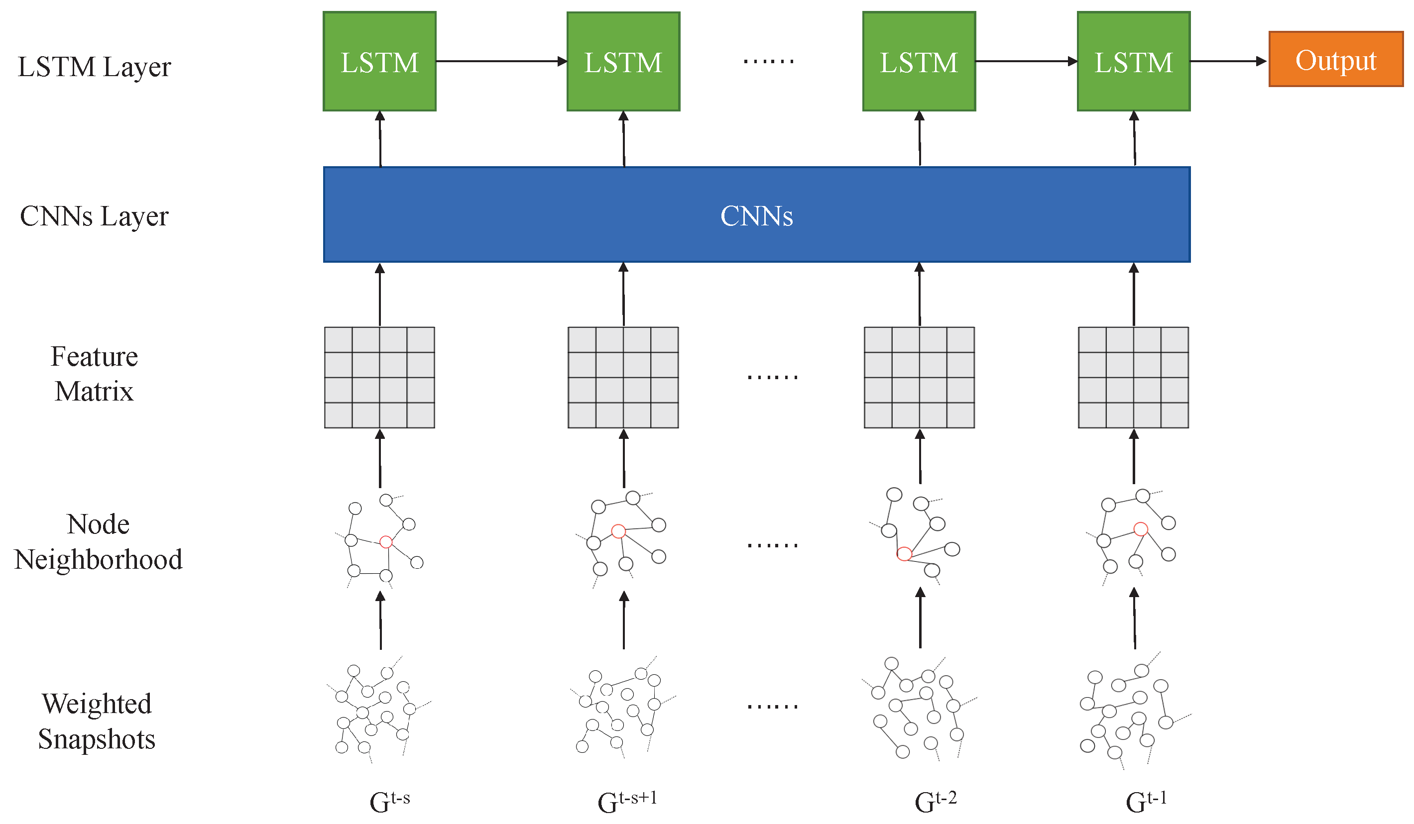
Figure 1. An illustration of DGCN.
Applsci 13 07272 g001
Figure 2. Unweighted snapshots and weighted snapshots: (a) Unweighted snapshots; (b) weighted snapshots, δ = 1 .
Applsci 13 07272 g002
Figure 3. A schematic diagram of training and predicting by DGCNs.
Applsci 13 07272 g003
Figure 4. The impact of the number of input snapshots s on final kendall τ .
Applsci 13 07272 g004
Figure 5. The impact of infection rate β on final kendall τ .
Applsci 13 07272 g005
Figure 6. The top 5% H R under different infection rate β .
Applsci 13 07272 g006
Table 1. Statistical properties of four real-world networks. N and M are the total number of nodes and edges, respectively. δ is the time interval (hours) used to divide networks and L is the number of snapshots.
NetworksNM δ L
Email986332,33416875
Contact27428,244169
DNC186539,6231256
UCI189959,8352458
Table 2. The training time (seconds) of four temporal networks with different s.
Networks s = 1 s = 2 s = 4 s = 8 s = 15 s = 30
Email69.1777.4594.46132.30195.10341.90
Contact21.5422.7328.0638.8758.55106.61
DNC128.01147.25175.50247.95362.78643.84
UCI126.32142.78176.30261.63385.58752.10
Table 3. The time cost of ranking nodes (seconds) on different networks.
NetworksDGCNN2V-LSTMS2V-LSTMTDCTK
Email2.460.080.0726.670.32
Contact0.090.040.041.200.06
DNC0.450.160.14132.710.37
UCI0.230.170.13140.740.36
Disclaimer/Publisher’s Note: The statements, opinions and data contained in all publications are solely those of the individual author(s) and contributor(s) and not of MDPI and/or the editor(s). MDPI and/or the editor(s) disclaim responsibility for any injury to people or property resulting from any ideas, methods, instructions or products referred to in the content.