Abstract
Direct-drive electro-hydraulic servo valves are widely used in the aerospace industry, in the military, and in remote sensing control, but there is little research and discussion on their performance degradation and service life prediction. Based on previous research, erosion wear is the primary physical failure form of direct-drive electro-hydraulic servo valves, and parameters such as opening, oil contamination, and pressure difference are used as influencing factors of direct-drive electro-hydraulic servo valves. Pressure gain and leakage are used as performance degradation indicators of servo valves, and multiple types of sensors are used for data monitoring. Experimental benches are arranged and verified through experiments. Based on the data and laws obtained from the experiments, the exponential smoothing algorithm and the ARIMA model algorithm were used to establish a prediction model for the servo valve, and the dynamic prediction of the performance indexes was carried out. The error calculation and analysis of the prediction results and the experimental results were then carried out using the Copula function and other mathematical knowledge to verify the accuracy and applicability of this prediction model. This study provides theoretical support and practical guidance for applying and designing direct-drive electro-hydraulic servo valves in industrial applications such as aerospace, sensor experiments, and remote sensing control.
1. Introduction
Direct-drive electro-hydraulic servo valves are an essential control element in both aerospace and remote control. In modern industrial control, fluid-hydraulic control or pneumatic control occupies the primary control strategy market, so the study and application of one of its essential control components, the direct-drive electro-hydraulic servo valve, is also a major research point.
For example, in the field of remote sensing, for the design of monitoring mobile scanning systems in thermal systems [1], control valves such as servo valves, as the leading equipment for the thermal components of the thermal system, have a non-negligible impact on the accuracy of the final scanning system. The Spanish scholar Freddy et al. [2] evaluated the performance of an urban park irrigation system where water consumption was used as the main argument factor. In contrast, water consumption was related to the control of the valve element of the servo valve, another great application of their research in conjunction with the evaluation system. In thermal power plants [3,4], servo valves, as the main components of their digital electro-hydraulic control systems, leak, and other failures are also one of the main causes of control system failure in thermal power plants. Saha et al. [5] have also studied servo valves used in fighter jet wing and robot control systems, combining simulations and experiments to verify their internal flow in such industrial applications. In aerospace and aircraft or missile control [6], where servo valves are widely used, their internal fluid conditions and pressure characteristics are also important influencing factors in such areas.
In addition, life prediction is closely related to the physical failure and degradation of components and is a significant focus of attention in both the aerospace and remote control sectors. For electro-hydraulic servo valve life prediction, most of them are applied to the Bayesian tracking method and others [7,8] for diagnosis and prediction. However, this relies mainly on models, mechanical components, or wear experience for analysis and does not lead to a regular diagnosis and projection method. The accuracy of the results has too large an upper and lower accuracy limit for routine use in the modern control industry. In recent years, more life prediction methods have been devised. Rommel et al. [9] proposed a load-based prediction method that combines multiple forces such as load, structural properties, and material properties through the specific use and industrial conditions of the system to which the part is subjected, which is then monitored to form a set of life prediction parameters. Scholars Aghajani Sepideh [10] and others have also proposed a new fatigue damage model for the life prediction of wind turbine blades that cascades and expands the various loss behaviors of the components. The process is also available in the ABAQUS software user material subroutine. Thelen Adam et al. [11] updated and extrapolated a novel mathematical model for the lifetime prediction of rechargeable battery cells, allowing the model to describe the evolution of the battery capacity decay trend while retaining its desirable characteristics such as uncertainty quantification. Doremus et al. [12] describe a method for life prediction from static fatigue measurements for life prediction from the plastic material of the part itself and suggest that its most critical factor is the assumed dependence of the time to failure on stress, and then validated the validity of their method. Kong Yu Sik et al. [13] in Korea combined the initial strain parameter method and the Larsen–Miller parameter method to study the remaining service life of automotive engine components made from the metallic material Alloy 718 at high temperatures. They experimentally verified the validity of such practices under high temperatures and continuous pressure at 550 °C to 700 °C. In addition, Yuan Li et al. [14] used computational fluid dynamics (CFD) and combined turbulence theory and microerosion principles to develop a physical model of the erosion suffered by a novel linear electro-hydrostatic actuator (LEHA) under high-frequency turbulent flow conditions, and explored the effect of the concentration of contaminated solids on erosion. Similarly, scholars Kun Zhang et al. [15] established a mathematical model of erosion wear for a conventional electro-hydraulic servo valve, using its structural wear combined with CFD theory, and discussed the effect of each structure of this electro-hydraulic servo valve on erosion wear and servo valve performance. However, the above methods are too dependent on the material properties of the components and the influence of the forces to which they are subjected and are analyzed purely from a physical or mechanical point of view. Such influences are not fully controllable in practical industrial applications, and the structural requirements for servo valves are limited and less universal, and therefore cannot be fully and universally applied in industry.
With the rise of the information age, there has been considerable development in intelligent data-driven processes and big data, and in particular an increase in the research and application of neural networks as a core strategy for machine learning and artificial intelligence, for example, which has led to an increase in the accuracy and precision of prediction results in terms of lifespan prediction. Scholars R. Talebitooti et al. [16,17] used a combination of non-dominated sorting genetic algorithms and first-order shear deformation theory to model the frequency-based acoustic properties of an elastic material core and its shell as a means of determining the loss of the object of study. Hongmei Liu et al. [18] of Beijing University of Aeronautics and Astronautics (BUAA) established fault and health observations, as well as performance degradation predictions for hydraulic servo systems based on Elman network observer and support vector regression (SVR). However, this algorithmic model is suitable for highly non-linear and non-stationary conditions and is less effective in the analysis and forecasting of time-series seasonal and even non-seasonal regularity data. In this research project, support vector machine algorithms have been used to predict the life of direct-drive electro-hydraulic servo valves, but the results are less effective than other algorithmic models, and the errors are greater. Others, such as Xingyan Yao [19], designed a system for monitoring and testing the service life of hydraulic shock absorbers in vehicles using various sensors, data acquisition cards, and Labview as a PC. However, such algorithms are good for fault diagnosis and monitoring, but how effective they are for predicting future trends is open to question. Siahpour Shahin et al. [20] from the University of Cincinnati, USA, proposed a migration learning method for lifespan prediction using consistency-based regularisation, which avoids the effect of missing data and finally validates its effectiveness experimentally. Wang Hang et al. [21] from Harbin Engineering University proposed a method that can be applied to the life prediction of electric valves in nuclear power systems by combining the advantages of convolutional encoders and long- and short-term memory neural networks in terms of depth and time breadth, respectively. This method allows for a parallel structure with neural network characteristics to be built between the input and output of the initial data. Sweta Bhattacharya et al. [22] used a deep-neural-network-based optimization model to predict the battery life of an IoT system and then implemented the moth flame optimization (MFO) algorithm to select the optimal data features before feeding this feature into the neural network model for life prediction. Ferreira Carlos et al. [23] also specifically address the relationship between lifespan prediction and neural networks and machine learning. Condition-based maintenance is proposed to perform daily maintenance according to the needs of machines and components, as well as predictive and health management using metrics to monitor the evolution of component wear. However, most of this series of neural networks combined with life prediction methods are based on the application of bearings, batteries, and so on. The combination of direct-drive electro-hydraulic servo valves is rarely applied, and the influence of different influencing factors, such as temperature and differential pressure, on their service life still needs to be better understood.
As can be seen from the above literature, there needs to be more research in the current industry on the performance degradation and life prediction of the spool sleeve of direct-drive electro-hydraulic servo valves, especially in combination with information age neural networks for their life prediction. In addition, it is unclear how the performance degradation and life prediction pattern of the direct-drive servo valve spool sleeve changes under different parameters such as differential pressure, flow rate, and opening degree. Since direct-drive electro-hydraulic servo valves are one of the core control elements in aerospace or remote control, further performance degradation and life prediction of the spool valve sleeve for direct-drive electro-hydraulic servo valves is of great significance in the whole field of electro-hydraulic industrial management, based on a previous study of the erosion and wear pattern of direct-drive electro-hydraulic servo valves [24]. This paper starts from a direct-drive electro-hydraulic servo valve, uses the performance degradation law obtained from the predecessor for experimental verification, then combines the experimental data to design a prediction model for the dynamic prediction of its performance degradation index, and finally obtains its law.
2. Development of a Servo Valve Prediction Model
2.1. Servo Valve Erosion and Wear Distribution
The residual particle impurities in the special oil will cause damage to the servo valve components, resulting in the servo valve mouth and other parts of the physical properties of change forming the erosion and wear phenomenon; it is effortless to reduce the primary function of the servo valve, resulting in the servo valve, because it cannot reach the designed performance indicator work mechanism severe attenuation. Therefore, the mathematical model of the erosion and wear characteristics of the servo valve was established directly in this paper using the mass and momentum conservation theorems of the previous study [24].
The medium oil flow through the servo valve orifice position encounters narrowing of the valve orifice structure, resulting in rapid attenuation of the flow beam, and oil flow speed in the approved period increases significantly, the result of the collision with the wall of solid particles in the region of the precipitation aggregation phenomenon, in comparison with other areas of granular impurities where the density is much larger, due to the narrowing of the valve orifice structure leading to the quick movement of the region of granular impurities, making the control surface of the valve orifice area sharp edge wear be pronounced, so the servo valve processing and production process needs to be optimized for the control surface of the valve orifice area in order to increase its ability to resist impact, usually on its surface to deal with physical methods. The wear on the sharp edge of the countersunk face and the sharp edge of the flank of the raised shoulder differed considerably and was relatively severe, with the angle of the jet as the oil passes through the valve opening being the main factor in this wear.
The expression for the relationship between the jet angle α and the valve opening x and the fit clearance Cr is as follows [25]:
As shown in Figure 1, the value of x is greater than Cr during regular operation of the servo valve, and the value of α for this operating condition lies between 60° and 70°. The trajectory of the granular impurities in the oil is consistent with the trajectory of the medium oil, so the geometric principle calculates the electro-hydraulic servo valve reliability change curve, and the impact angle of the granular impurities on the end face of the sink groove is basically fixed. Generally, the value is controlled between 20°and 30°, and the impact angle of the granular impurities on the side of the convex shoulder is also basically set, generally controlled between 60° and 70°. We used θ as a proxy for the angle of impact between the trajectory of solid contamination particles and the wall of the spool sleeve. According to the range of impact angle values listed in the literature [18], it is shown that when the value of the impact angle θ of the particle against the wall is fixed between 20° and 30°, the corresponding value of the impact angle function f(θ) ranges between 0.8 and 1; when the value of θ is fixed between 60°and 70°, the corresponding value of f(θ) ranges between 0.4 and 0.5 in the region. According to the erosion rate calculation formula [18], the erosion wear rate Re is proportional to f(θ) at constant working conditions. The calculation results show that the wear rate of the sharp edge of the control surface of the sinker is very different from the wear rate of the sharp edge of the control surface of the convex shoulder.
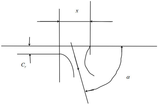
Figure 1.
Jet angle of the fluid flow at the valve port.
In summary, numerous factors, such as the physical characteristics of the particulate impurities and the valve opening, are the main causal factors for the erosion and wear of the slide valve. These causal factors affecting the erosion and wear of slide valves are examined separately in the primary research literature [24], with each causal factor being specifically analyzed for its formation.
2.2. Rationale for Expectancy Projections
2.2.1. Theoretical Foundations of Exponential Smoothing Forecasting and Fusion Prediction
Exponential smoothing is a time series forecasting method for univariate data with a wide range of applications for the predictive analysis of data with systematic genera and with seasonal components and is one of the oldest and most studied time series forecasting methods. It is most effective when the time series values follow an asymptotic trend and show seasonal behavior (i.e., when the values follow a repeating periodic pattern over a given number of time steps).
Exponential smoothing uses an exponential window function to smooth time series data. In a simple moving average, past observations have the same weight, whereas the exponential function is used to specify weights that are exponentially decreasing over time.
In the exponential smoothing process, past observations are proportionally weighted to the data obtained geometrically decreasingly. The prediction result is based on the weighted average produced by the exponential smoothing method, with an exponentially decaying trend in the weights obtained based on the difference in time between the data obtained immediately and the current value. That is, the closer the observation time, the higher the relevant weight. Exponential smoothing methods are equivalent to peer-to-peer methods and are applied interchangeably with ARIMA (autoregressive integrated moving average model) methods for time series forecasting. These forecasting methods provide error, trend, and seasonal characteristics to construct models.
There are three main types of exponential smoothing time series forecasting methods: simple methods that assume no systematic structure, extensions that deal explicitly with trends, and state-of-the-art methods that support seasonality.
The primary use of single exponential smoothing (SES), also known as simple exponential smoothing, is a method for time series forecasting of univariate data. Set the smoothing factor to a. This smoothing factor constrains the observations for the previous time step and can have an effect on the rate of exponential decay. a is usually set to a value between [0, 1]. The range of values implies whether the model is primarily concerned with recent past observations or whether it will take more history into account when making predictions.
Exponential smoothing is a simple but powerful method for predicting time series. Exponential smoothing is also used as a building block by many other models. Compared to simpler forecasting models such as simple or moving averages, exponential smoothing models have two advantages: one is that the weight of each observation decreases exponentially over time. This compares favorably with a moving average model that assigns the same weight to all relevant historical months. In addition, the effect of outliers and noise is less than that of using the plain method.
The basic idea of the exponential smoothing model is that in each period, the model learns a little from the most recent demand observation and remembers the last forecast it made. The final forecast populated by the model already contains part of the previous demand observation and part of the previous forecast. Therefore, this previous forecast includes everything the model has learned so far based on the demand history. The smoothing parameter (or learning rate) a will determine the importance of the most recent demand observation. It is expressed as follows:
where a is the ratio (or percentage) of importance that the model will assign to the most recent observation of the historical importance of demand. adt−1 denotes the previous demand observation multiplied by the learning rate. It can also be expressed that the model attaches a certain weight a to the last demand occurrence. (1 − a)ft−1 indicates how much the model has remembered from previous predictions. This is where the recursive magic happens, and ft−1 itself is defined as part of dt−2 and ft−2. In the experimental data sample of this article, the observed value ft represents the predicted value of our servo valve performance parameter—pressure gain or leakage at time t. dt represents the experimental data value of the performance parameter at time t.
There is a trade-off between learning and memory and between reactivity and stability. If a is high, the model will place more emphasis on recent demand observations (i.e., the model will learn quickly) and will respond to changes in demand levels. However, it can also be sensitive to outliers and noise. On the other hand, if a is low, the model will not notice rapid changes in levels, but will also not overreact to noise and outliers.
Once the historical period has been left, forecasts for future periods must be populated, and the final projections (those based on recent demand observations) are extrapolated into the future. If f{t*} is defined as the last forecast that can be made on the basis of demand history, just ft≥t* = ft*, this simple exponential smoothing model is more flexible than the moving average model because it is more intelligent in its weighting of historical demand observations.
For the exponential smoothing algorithm, its exponential smoothing statistic lies mainly in the α-value. Moreover, for the value of α, we can turn to the planning solution of the Excel software. Excel is used to record the servo valve pressure gain and leakage performance parameter data obtained from the next chapter of the experiment and combined in the same data table, and then the predicted value of the data for exponential smoothing calculation, the predicted value by ft = α * dt−1 + (1 − α) * ft−1, is obtained, where d indicates the actual data value and f indicates the predicted value, and then dt − ft is used to get the error value. Then, the error is squared and the average of the whole set of working conditions data is sought to obtain the mean squared error MSE; a smaller MSE means that the value of α is more appropriate at this time, and thus there is a higher accuracy of the exponential smoothing model. Finally, the data column of the Excel software is used to simulate the analysis option in the planning solution, the target solution goal is set to the minimum value of the MSE, the variable cell is set to the value of α, the requirement is set to make 0 < α < 1, and then the solution is clicked on. After several calculations of pressure gain and leakage, we found that at α = 0.812, the relative MSE of each data point was 0.001070273, so we took the weight parameter α of 0.812 as the parameter requirement in the exponential smoothing model.
Fusion forecasting refers to the technique of combining the results of multiple forecasting models to generate more accurate and stable forecasts. In practice, we often use several different forecasting models to make predictions, such as models based on different algorithms, models with other parameters, and so on. Each of these models has its own strengths and weaknesses, so combining their results can compensate for the shortcomings of individual models and improve prediction accuracy and robustness.
2.2.2. ARIMA Theoretical Foundations
The promising ARIMA model, also known as the Box–Jenkins methodology, consists of a series of activities for identifying time series data, as well as estimating and diagnosing ARIMA models. In an ARIMA model, the future value of a variable can be understood as being the correlated property of past values and past errors, expressed by the following equation [26]:
where Yt is the actual value; t and δ are the random errors at t; b is the coefficient; and p and q are integers, often referred to as the autoregressive and moving average, respectively. Building an ARIMA predictive model includes model identification, parameter estimation, and diagnostic checks.
The main advantage of ARIMA forecasting is that it only requires data on time series. This function is suitable if a large number of time series are to be predicted, in addition to avoiding some of the problems that tend to arise in multivariate models, for which the timeliness of the data is also essential. If a large structural model is constructed containing variables that are only released over a long period, forecasts using this model are conditional forecasts based on the prediction of unavailable observations, thus increasing the potential for forecast uncertainty.
The ARIMA(p,d,q) model is a linear model suitable for dealing with random series. It originates from the autoregressive model AR(p), the moving average model MA(q) and the association of AR(p) and MA(q), and the ARMA(p,q) model. ARIMA(p,d,q) models are usually organized in the following form:
where p,q is the order of the AR and MA models and d is the number of serial differences. p, d, q are all integers. is the estimated residual for each time period. If the model is optimal, it should be independent and distributed as a normal random variable with a mean of 0. is the variance of the residuals.
where and are polynomials of degree p and q in B. B is the back-shift operator.
The data prediction of the experimental data obtained in Section 3 was carried out by means of exponential smoothing algorithm models and ARIMA algorithm models, among others. The data for each performance parameter under each set of operating conditions was divided into two parts, the training set and the test set, by time before and after, e.g., the first 70% of a certain data was classified as the training set and the last 30% was classified as the test set. We then used the prediction model to make subsequent predictions, compare the predicted results with the remaining 30% of the test set data, and perform error calculations for model validation.
2.2.3. Supervised Machine Learning
Sliding Time Window
Sliding time window analysis of time series models is often used to assess the stability of the model over time. When statistical models are used to analyze inter-series data, the model’s parameters are usually set to be constant and do not change over time. However, the environment often changes so much that it is impossible to assume that the model’s parameters are constant. A common technique for assessing the stability of model parameters is to calculate parameter estimates over a rolling window of fixed size in the sample. If the parameters are constant throughout the sample, then the forecast on the rolling window should be similar. If the parameters change at some point during the sample, then the rolling estimates should capture this instability.
Historical data are used to assess stability and forecast accuracy. Backtesting typically works in the following way: the recorded data are initially divided into an estimation sample and a forecast sample. The model is then fitted using the estimation sample, and an h-step ahead forecast is made for the forecast sample. The h-step ahead prediction error can be formed as the data for which the prediction is made is observed. A given increment then slides forward the estimation sample, and the estimation and prediction exercise is repeated until no more h-step predictions can be made. The statistical properties of the set of h-step ahead prediction errors are then summarized and used to assess the adequacy of the statistical model.
Feature Selection
A common problem in machine learning is identifying a set of relevant features to build a classification model. The most crucial feature selection task is eliminating inappropriate and redundant data, which helps improve the performance of learning algorithms. Feature selection (FS) is crucial in machine learning; it is the primary method for collecting and categorizing data and it occupies an extremely important place in research areas such as computer pattern recognition. Four main benefits of FS are the elimination of inappropriate and unnecessary features, making data mining tasks easier, improving accuracy, and simplifying and making conditional models easier to understand.
The simple variable importance metric used in the tree-based integration approach is to count only the number of times each variable is selected by all individual trees in the integration. A more refined variable importance metric consists of the improved (weighted) average of the splitting criteria generated by individual trees for each variable. An example of such a classification metric is the “Gini importance” available in random forest implementations. “Gini importance” describes an improvement in the “Gini gain” splitting criterion.
The most advanced variable importance measure available in random forests is the “permutation accuracy importance” measure. The basic principle is as follows: by randomly ranking the predictor variable Xj, its original association with the response Y is broken. When the Xj replacement variable is used with the remaining un-replaced predictor variables to predict the response, the prediction accuracy (i.e., the number of correctly classified observations) is significantly reduced if the original variable Xj is associated with the answer. Thus, a reasonable measure of variable importance is the difference in prediction accuracy before and after the replacement of Xj.
For variable selection purposes, the advantage of the random forest ranking accuracy importance measure over univariate screening methods is that it covers the effects of each predictor variable individually as well as multivariate interactions with other predictor variables.
Feature selection is selecting relevant features in a dataset based on a subset of features obtained from the initial set of features according to specific feature selection criteria. The main function of this process is to compress the data and analyze them accordingly, removing certain features from the data that have little relevance and semantic overlap. Feature selection techniques can pre-process learning algorithms, and good feature selection can achieve more accurate purposeful learning, improve learning efficiency, and maximize learning outcomes. Therefore, the dimensionality reduction method can be performed by first completing the feature selection link and then extracting the obtained features. Unlike feature selection, feature extraction usually requires transforming the original data into parts with strong pattern recognition capability. The original data can be regarded as features with weak recognition capability.
Support Vector Machines (SVM)
The basis for support vector machines (SVMs) was developed by Vapnik (1995) and they are widely used due to their many advantageous features and empirical nature. The method has structural risk minimization (SRM) properties that are more advanced than the traditional empirical risk minimization (ERM) principles used in neural networks. SRM minimizes the upper bound on the expected risk, while ERM minimizes the error in the training data. The differences give the SVM more excellent generalization capability, which is the goal of statistical learning. Support vector machines were developed for solving classification problems, but recently they have been extended to the field of regression problems. In the literature, the terminology of SVMs can be confusing. The term SVM allows for a concise classification of support vector methods, and support vector regression covers the regression of support vector methods. Throughout this paper the term SVM will refer to classification and regression methods. Support vector classification (SVC) and Support vector regression (SVR) will be used to specify the minimization principle. By definition, support vector machines are divided into support vector classification machines and support vector regression machines. Support vector classifier is used to study the quantitative relationship between input variables and dichotomous variables and classification prediction. It takes the training set as the data object, analyzes the quantitative relationship between input variables and dichotomous output variables, and implements the prediction of the output variable class for new data. Support vector regression machines are used to study the quantitative relationship between input variables and numerical output variables and regression prediction. It also takes the training set as the data object and finds the maximum bounded regression plane by analyzing the quantitative relationship between input variables and numerical output variables to achieve a robust prediction of the value of the newly observed output variables. Support vector machines are an extension of algorithms based on the statistical learning theory that includes the VC dimensional theory and structural risk minimization principles and is a supervised learning method. Compared to other neural network regressions, the use of support vector machines to estimate regression functions has three distinct features. Firstly, the SVM estimates the regression using a linear part of special attributes in a high-dimensional space. Secondly, the SVM completes the regression estimation by risk reduction, wherein the risk is evaluated using Vapnik’s insensitive loss function. Thirdly, the principle of the set of functions used by support vector machines is that the composition of regularization terms derived from empirical error and structural risk minimization must be followed.
Support vector machines (SVMs) overcome the inherent flaws of neural networks, such as local minima, over-learning and architectural selection, and over-reliance on experience for types. In its simplest and most linear form, an SVM is a hyperplane that divides a set of positive samples from a collection of negative samples with maximum margins. In the attribute-deterministic case, the margin is defined by the distance from the hyperplane to the nearest positive and negative sample.
Decision Tree
A decision tree is a binary tree with two types of nodes. Some nodes are leaf nodes; they contain class labels or predictions. Other nodes are internal; they have functions for splitting the original sample. In internal nodes, attributes are often compared to a specific value, which implies using simple threshold rules. However, this does not exclude the possibility of using complex multidimensional functions. These functions help to construct complex partition surfaces, but they are rarely used in practice because they make decision trees relearn more quickly. Machine learning algorithms always have some parameters and settings on which the efficiency of these methods depends. Decision tree learning algorithms have their own set of settings and parameters, which determine the nature of the algorithm. This means that we get a different algorithm to learn the decision tree by changing these parameters.
Random Forest
Over the past two decades, random forest (RF) classifiers have received increasing attention due to the excellent classification results and processing speed achieved. RF classifier uses predictions from a collection of decision trees to produce reliable classifications. Furthermore, the classifier can successfully select and rank the variables with the greatest ability to distinguish between target categories. This is an essential asset as the high dimensionality of remotely sensed data makes the selection of the most relevant variables a time-consuming, error-prone, and subjective task. Many studies have systematically investigated the use of RF classifiers for hyperspectral data classification and enhanced thematic map (ETM+) or multispectral scanner (MSS) land cover (LC) classification and digital elevation model (DEM) data. However, publications have yet to specifically summarize the use of such versatile and efficient classifiers in different application scenarios.
A random forest (RF) classifier is an integrated classifier of a decision tree, which is generated from a randomly selected subset of training samples and variables. This classifier has become popular in remote sensing due to its classification accuracy. The overall objective of this work is to review the use of RF classifiers in remote sensing, which are superior in dealing with high-dimensional data and multicollinearity problems, avoiding the sensitive problem of overfitting and enabling fast classification. However, it is susceptible to sampling design. The variable importance (VI) measure provided by the RF classifier has been widely used in different scenarios, such as reducing the dimensionality of hyperspectral data, identifying the most relevant multi-source remote sensing and geographic data, and selecting the most appropriate season to classify a specific target class. Less common uses of the classifier need to be further investigated, such as for sample proximity analysis to detect and remove outliers from training samples.
Xgboost
Xgboost is an acronym for the eXtreme Gradient Boosting package. It is an efficient and scalable implementation of the gradient boosting framework. The package includes efficient linear model solvers and tree-learning algorithms. It supports the learning of a wide range of objective functions. The box is scalable and allows the program developer to determine the objective function independently.
Xgboost is a supervised learning algorithm that implements a process called boosting to produce accurate models. Supervised learning is inferring a predictive model from a set of labelled training examples. This predictive model can then be applied to new unseen examples. Supervised learning can be used to solve classification or regression problems.
2.2.4. Copula Function Theory
Copulas is a tool for modeling the dependencies of several random variables. The primary purpose of copulas is to describe the interrelationship of several random variables. This paper is dedicated to the use of the Copula function, the joint probability density distribution, to describe the relationship between the two variables, the predicted values and the test set data. The theory of Copula functions has been rapidly developed in statistics and has provided the theoretical basis for evaluating system reliability problems.
All functions satisfying a particular condition are Copula functions [27]. The density function of the multivariate joint distribution is decomposed, and the value is obtained by multiplying the decomposed n-edge distributions with the Copula function.
The multivariate Copula function C(u1,……,un) is a function that satisfies the following conditions:
- A.
- The domain of definition of the function C(u1,……,un) is [0, 1]n;
- B.
- The function C(u1,…,un) is zero-based and n-dimensionally increasing;
- C.
- Any ui∈[0,1], i = 1,2,……,n, satisfies:C(1,…,1,ui,1,…,1) = ui;C(u1,…,ui−1,0,ui+1,…,un) = 0;
- D.
- If u1,…, un are independent, then: C(u1,…, un) = u1…un.
Construct the joint distribution from Sklar’s theorem for multivariate Copula functions, defined for Sklar’s theorem as assume that F1(x1),F2(x2),…,Fn(xn) is a one-dimensional continuous distribution function and let u1 = F1(x1), u2 = F2(x2),…, un = Fn(xn), then u1,u2,…,un are uniformly distributed obeying [0, 1], i.e., C(u1,……,un) belongs to the marginal distribution and obeys the joint distribution function of [0, 1]. Let F(x1,x2,…,xn) be a joint distribution function with an edge distribution function F1(x1),F2(x2),…,Fn(xn), then there exists a multi-dimensional Copula function C(u1,……,un) that can connect the starting edge distribution function F1(x1),F2(x2),…,Fn(xn) to the joint distribution function F(x1,x2,…,xn), as expressed by the following equation:
In summary, the Sklar theorem for multivariate Copula functions is a combination of multiple random variables, i.e., they can be associated by their respective marginal distributions. Copula functions complete the proof of the association between the variables, different Copula functions prove the corresponding association, and the relevant parameters of the Copula function prove the data on the degree of association.
Servo Valve Reliability Model Based on Copula Function
The construction of the copula model in this paper is divided into the selection of the copula and the construction of the model:
- A.
- copula selection
In this paper, the principle of copula selection based on non-parametric kernel density estimation is used, which means that the non-parametric kernel density method is used to evaluate the edge distribution of the sample. The copula functions that can describe the correlation between failure modes are obtained from the copula functions after screening. The parameter determination values in the copula are calculated based on the copulafit function. Then, the Euclidean squared distance between these copula functions and the empirical copula functions is filtered to finally select the optimal copula function.
- B.
- Computational model construction
Let Fxi−1 denote the inverse function of Fxi(1,2,…,n). Then, Equation (10) can also be expressed as
where ui = Fxi(1,2,…,n); u = (u1,……,un).
According to what Equation (11) deduces when the edge distribution is determined, the copula function can be formulated to construct the joint distribution function. Let the number of failure modes of the system be k. The process can be expressed as
where Ej = |Zj(X1,X2,…,Xn) ≤ 0| denotes that there is a jth failure mode, and then the probability of failure can be expressed as
The form of direct-drive electro-hydraulic servo valve failure studied in this paper can be further expressed as follows:
Reliability Analysis of Degraded Systems Based on Copula Functions
The probability density function f(x) captures the probability that a random distribution sample is equal to x. For example, the formula for the probability density function of a standard normal distribution is as follows:
where the probability density function returns not probability but “relative likelihood” and can take values in the interval [0,∞); however, the integral of the probability density function from −∞ to ∞ must be equal to 1. The integral of the probability density function F(x) is a cumulative distribution function and is expressed as follows:
where probabilistic integral transformations are an essential part of Copula with respect to supposing a random variable, x, comes from a distribution with a cumulative density function, F(x). Then, a lucky variable, Y, can be defined with the following expression:
This formula proves that Y follows a uniform distribution over the interval [0.0,1.0]. The integral probability transformation shows that for X, if a continuous random variable F(x) with a cumulative distribution function, then the random variable Y = F(x) obeys a uniform distribution over the interval [0.0,1.0]. The formula for its proof is as follows:
Let the random variable Y be Y = F(X), where X is another random variable, then
where there is a cumulative distribution function of a random variable, so that Y = F(X) follows a uniform distribution over the interval [0.0,1.0].
If {x1,x2,…,xn} is a random sample from X, then the value {Fx1,Fx2,…,Fxn} is a random sample obeying a uniform distribution. The key to the copula function is that the edge distribution can be modeled independently of the joint distribution. The copula-based modeling approach can be, in turn:
- a.
- Independently modeled based on servo valve pressure gain (Mpa/mm), internal leakage (L/min) data;
- b.
- Converted them to a uniform distribution using the integral probability transformation described above;
- c.
- Modeled the relationship between the transformed variables using the copula function.
2.2.5. Joint Probability Density Distribution
This paper uses the two-dimensional joint probability density distribution as the study sample, and its calculation method is divided according to the different correlation coefficients used. The construction method based on the Pearson correlation coefficient is called the approximate method P; the other one is based on the Spearman correlation coefficient, called the approximate method S.
Approximate Method P
Suppose the Pearson’s correlation coefficient between variables Y1 and Y2 is rPY, then the joint probability density functions of variables Y1 and Y2 are f1(y1) and f2(y2), respectively. The joint probability density function of the variables Y1 and Y2 can be found using the Nataf model, which is expressed by the following equation:
where Φ(x)is denoted as the probability density function of a one-dimensional standard normal variable, and Φ2(x1,x2:rPP,x) is the probability density function of a two-dimensional standard normal distribution with a Pearson correlation coefficient of rPP,x.
Approximate Method S
Suppose the Spearman correlation coefficient between variables Y1 and Y2 is rS,Y, and the Spearman correlation coefficient between variables X1 and X2 is rS,X; according to the definition, we can get
The joint probability density function of the variables Y1 and Y2 constructed by the approximation method S can be expressed as
where Φ2(x1,x2:rPP,x) is the probability density function of a two-dimensional standard normal distribution with a Pearson correlation coefficient of rPP,x. The Pearson correlation coefficient between variables X1 and X2 is rPP,x. The equation for the relationship between rPP,x and Spearman correlation coefficient rS,Y is expressed as
Using both approximation methods, the reliability of the life prediction system can be effectively calculated to a reasonable level of accuracy. If the probabilistic information associated with a lifetime prediction system needs to be more comprehensive, it is more convenient to use an approximation to evaluate its accuracy. On the other hand, if the relevant probabilistic information is more complete, it is preferable to construct joint probability distribution functions for the variables using simpler approximations. In theory, these methods can ignore the dependence of probabilistic data and allow accurate evaluation of the lifetime prediction system, albeit with a slightly different computational procedure.
3. Dynamic Prediction of Servo Valve Performance Degradation
3.1. Servo Valve Erosion and Wear Test
The specific test design includes five parts: test hardware configuration, environmental condition setting, test typical operation, test data acquisition design, and data post-processing.
3.1.1. Test Hardware Configuration
A schematic diagram of the servo valve spool erosion and wear test system is shown in Figure 2 below. The hydraulic pump 2 is the main pump for the entire flow control system and supplies the working medium or hydraulic oil. Thermometer 3 monitors the initial temperature of the hydraulic fluid and allows changes in the fluid temperature to be monitored at any time during the experiment. Two filters, 4 (1) and 4 (2), are used to filter large-diameter solid particles from the oil circuit. The main function of relief valve 5 is to regulate and maintain a constant pressure throughout the hydraulic system, so its main object of work is the source of the supplied fluid—the hydraulic pump 2. In addition, the four pressure gauges 6 (1)–6 (4) are used to check the pressure at the four oil ports of the servo valve and are connected to a pressure sensor that transmits the pressure signal to the computer. The throttle 8 regulates the system oil flow according to the experimental situation and can also be seen as a specific load acting on the servo valve of the measured flow. Finally, the two shut-off valves 9 can assume the on–off status of the servo valve’s return port for the measured flow. When 9 (1) pathway and 9 (2) disconnect, representing the normal working fluid state of the experiment, that is, the measured flow servo valve erosion and wear experiments are constantly carried out. When the flow servo valve 7 is in the neutral position, 9 (1) is disconnected and 9 (2) is open, the flow meter 10 can be used to detect the zero leakage of the flow servo valve, and the flow meter can be connected to the flow sensor so that the leakage signal can be input to the computer.
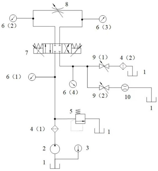
Figure 2.
Schematic diagram of the servo valve erosion and wear test system: 1—oil tank; 2—hydraulic pump; 3—thermometer; 4—filter; 5—relief valve; 6—pressure gauge; 7—direct-drive electro-hydraulic flow servo valve under test; 8—throttle valve; 9—shut-off valve; 10—flow meter.
Figure 3 below shows the spool sleeve wear test rig, which includes a pump source, servo valve, flow meter, throttle valve, globe valve, heat exchanger, pressure gauge, thermometer, and associated piping system.
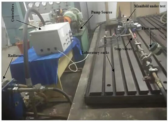
Figure 3.
Spool valve sleeve wear test rig.
(1) Hydraulic pump source: the hydraulic pump source used in this test has a rated pressure of 20.6 MPa and a rated flow rate of 100 L/min.
(2) Servo valve under test: the servo valve used in this experiment has a maximum flow rate of 30 L/min.
(3) Flowmeter: according to the rated flow rate of the system and the requirements of the pipeline system, this experiment used the model LWGYB-25 turbine flowmeter, with a range of 1 to 30 m3/h and an accuracy level of ±0.5.
(4) Throttle valve: in this experiment, throttle valve is equivalent to a flow control valve, and its requirements are low, so this experiment used the Shandong Taifeng hydraulic production model DVP-12 throttle valve.
(5) Globe valve: according to the function of the globe valve in this experiment and the requirements of the pipeline system, we chose the model CJZQ-H20L ball core globe valve, whose nominal pressure is 20.6 MPa and nominal diameter is 20 mm.
(6) Cooler: the test system was used in the BR005 type plate radiator; its design pressure is 1.3 MPa, and the design temperature is 150 °C, with heat transfer area of 6 m2.
(7) Pressure gauge: The pressure gauge used in this experiment is a shock-resistant pressure gauge, and the accuracy level of the pressure gauge is 1.6, where the range of the pressure gauge at the P, A, and B ports is 0 to 30 MPa and the range of the pressure gauge at the T port is 0 to 2.5 MPa. The pressure sensor was placed and connected in the pressure gauge.
This test considered that the pressure gain and leakage changes are caused by the erosion and wear of particles on it, so this experiment adopted the method of real-time recording of pressure gain and leakage changes by the sensor incoming signal computer. The aim of this experiment was to test and record the changes in the performance parameters of direct-drive electro-hydraulic servo valves as the operating time increased. The performance parameters are the characteristics of an instrument and the device itself. For example, in the case of an air conditioner, its heating, cooling, power consumption, etc., are its performance. With this in mind, we selected the pressure gain and leakage of the servo valve performance as our experimental test parameters.
3.1.2. Design of Experimental Conditions
- Oil contamination level
According to GJB 420B-2015 “Classification of solid contamination in aviation working fluids” [28], the classification was based on the size, particle number, and distribution of solid contaminants in the fluid, as well as the content of solid contaminants per unit volume of working fluid. The standard denotes specific particle size ranges by the letters A, B, C, D, E, and F. The solid contamination is classified into 15 classes according to the maximum limiting number of particles in these six size ranges contained in 100 mL of working fluid.
In this test, the physical failure model was simplified and the diameter of the maximum number of solid particles in the fluid was used to reflect the different fluid contamination levels. Considering the actual application environment of DDV, four different contamination levels of hydraulic fluid were proposed in this test: GJB420B-6, GJB420B-7, GJB420B-8, and GJB420B-9.
- 2.
- Opening degree
The simulation data showed four different openings of 0.1 mm, 0.2 mm, 0.3 mm, and 0.4 mm, which were selected.
- 3.
- Differential pressure
As the opening and differential pressure together affect the flow rate of the valve and the flow rate of the inlet, the differential pressure also needs to be taken into account. In view of the limitations of the experimental conditions, four different differential pressure conditions of 14 MPa, 16 MPa, 18 MPa, and 20 MPa were selected.
The entire orthogonal experimental working conditions are shown in Table 1 below. According to GJB3370-1998 “aircraft electro-hydraulic flow servo valve general specifications” [29], the total life of the servo valve needed to have 600 Fh for its high pollution test, so for each sample test for 500 h, every 50 h between the disassembly of the spool valve sleeve, there was cleaning and debridement treatment. Because the liquid oil temperature is difficult to control during the experiment, the oil temperature was not used as one of the experimental conditions for the time being. The initial oil temperature was set at 35 °C, which is commonly used in the industry.

Table 1.
Table of orthogonal experimental conditions.
3.1.3. Basic Test Procedure
Based on the test system built for this test and the purpose of the test, the specific test procedures are listed below:
(1) Check whether the hardness and size of the sleeve spool of the servo valve meet the requirements and install the valve into the test bench if the conditions are met.
(2) Install the servo valve under test in the test system, throttle valve 8 is completely closed, stop valve 9 (2) is closed, and stop valve 9 (1) is opened; start hydraulic pump 2, adjust the pressure of relief valve 5 to the rated pressure of the servo valve; test whether the leakage amount inside the valve under test meets the requirements; after the test is completed, stop the hydraulic pump.
(3) Throttle valve 8 is fully open, stop valve 9 (2) is available, stop valve 9 (1) is closed, and the servo valve port under test is fully open; start hydraulic pump 2 and adjust relief valve 5 and throttle valve 8 until the flow meter is at the specified flow rate under the test profile.
(4) Apply control signal and change the direction of the servo valve every 1 h interval so that the wear on both sides of the spool is balanced and remove the spool valve sleeve for the cleaning and drying process every 50 h of operation.
(5) Repeat step 4 until the test time reaches 500 h, then stop the test of the sample. Replace the sample and start the next stress profile test.
3.1.4. Experimental Data Collection Design
(1) Collection interval and test time
The sampling interval is 50 h per cycle, and the data signal is monitored by the computer every 500 s weekly.
(2) Data collection content
(1) Recording of test environment conditions
Before each test, the test environment conditions include test environment temperature and humidity, test temperature, oil contamination, flow rate, test operator, etc. Test time includes test start time, a sampling interval of each test, etc.
(2) Determination of the initial value of the experimental material performance parameters
In this test, the change in pressure gain and leakage volume is used to express the change in erosion and wear during the work of the spool valve sleeve, which in turn characterizes the performance degradation process of the spool valve sleeve, so the pressure gain and leakage volume values at the initial moment of the spool valve sleeve need to be measured.
(3) Data recording during the test
The spool valve sleeve is dismantled at certain intervals, cleaned, and dried and then tested and measured again, as well as the sampling time, test conditions, and other parameters, and then the spool valve sleeve is installed and tested again as required.
3.1.5. Experimental Data Collection Design
The leading cause of failure of the spool sleeve is erosion and wear; therefore, the pressure gain and leakage of the spool sleeve will gradually change during the degradation process due to friction and wear, so the pressure gain and leakage were chosen as the performance degradation indicators for erosion and wear of the spool sleeve in this test. To obtain the degradation curve throughout the test, pressure and flow sensors need to be connected so that the computer can always monitor the parameter signals.
3.2. Preliminary Analysis of Data
Pressure gain is an important concept that is often used to describe the responsiveness of a particular system under different operating conditions. In some cases, pressure gain can vary with time and therefore needs to be monitored and analyzed. This article provides details on the variation of pressure gain with time under different operating conditions.
Firstly, we needed to understand the definition and meaning of pressure gain. Pressure gain is the rate of change of pressure at the output of a system for a given input signal. In some cases, the pressure gain of a system may change over time due to different operating conditions. This means that the system may have different response capabilities at different points in time. It is therefore important to understand the pattern of pressure gain over time under different operating conditions to optimize the performance and stability of the system.
In practical applications, it is important to monitor the trend of pressure gain under different operating conditions. By monitoring and analyzing the pressure gain, we can better understand the performance and stability of the system and make adjustments and optimizations accordingly. For example, in some cases, we may need to increase the responsiveness of the system to accommodate changes in external loads. In this case, we can increase the pressure gain by adjusting the system parameters to increase system responsiveness.
In summary, the pattern of pressure gain over time under different operating conditions has an important impact on the performance and stability of the system. Understanding these patterns and monitoring and analyzing them accordingly can help us optimize the system’s performance and stability and thus better suit the application’s requirements. The variation of pressure gain with time for different operating conditions is shown in Figure 4 below:
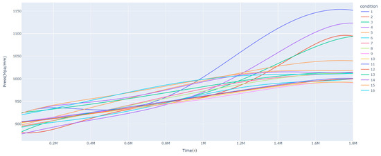
Figure 4.
Pressure gain variation graph.
As shown in Figure 4, we can see the trend of pressure gain over time for different operating conditions. As can be seen from the graph, the trend of pressure gain changed differently under other operating conditions. For example, the pressure gain for condition 1 showed a clear upward trend in the entire cycle, while the pressure gain for condition 10 did not show a clear upward trend. This indicates that the servo valve aged faster in condition 1 and slower in condition 2 during this period. The reasons for these trends may have been due to dynamic changes within the system caused by different operating conditions, such as oil contamination, differential pressure, or openness; changes in external loads; or changes in other factors.
In addition, because servo valves are a commonly used control element, they are widely used in hydraulic systems. During use, leaks may occur inside the servo valve, resulting in reduced performance and increased system energy consumption. Therefore, it is important to monitor and analyze the variation pattern of the internal leakage of servo valves under different operating conditions over time. In this paper, we introduced in detail the internal leakage of servo valves under different working conditions with time. The internal leakage of a servo valve is the amount of leakage between the spool and the valve seat, which is usually used to describe the sealing performance of a servo valve. The internal servo valve leakage amount may change over time under different operating conditions. This may be due to factors such as wear of the servo valve’s internal oil seal, the material’s aging, etc. Therefore, it is important to understand how the internal leakage of servo valves varies with time under different working conditions to ensure the performance and stability of the system. As shown in the figure below, we can see the trend of the internal leakage of the servo valve under different working conditions with time. From the graph, we can see that the trend of the internal leakage of the servo valve was different under different working conditions. The variation of servo valve internal leakage over time under 16 sets of experimental conditions is shown in Figure 5 below:
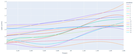
Figure 5.
Leakage variation graph.
As shown in Figure 5, we can see that some of the conditions had a faster increase in leakage, indicating that they were more affected by erosion and wear. For example, the groups of conditions with greater oil contamination showed more dramatic changes in leakage than other conditions with the same or similar conditions, but lower oil contamination. Combined with the above pressure gain and leakage data analysis graph, it is easy to see that, according to the different working conditions of the servo valve, the impact of changes in pressure gain and leakage was also different. The most noteworthy of these was that with little difference in other influencing factors, the influence of oil contamination had the greatest impact on the change in servo valve performance, followed by differential pressure and then openness. In terms of the overall trend of servo valve performance, pressure gain and leakage were generally slow to increase as the work progressed. The reason for this is that as the servo valve work is continually affected by erosion and wear, especially for the servo valve itself, the sharp edges and square holes of such structures are worn, so the internal leakage of the servo valve will increase and the pressure will be easier to build up, resulting in an increase in pressure gain.
Table 2 below lists the statistics relating to internal leakage and pressure gain.
Table 2.
Leakage and pressure gain statistics table.
3.3. Dynamic Prediction of Performance Indicators
In Section 2.2.1, we explained the theory of the exponential smoothing model, and in this section, we use the pressure gain or internal leakage of the servo valve as a one-dimensional time series for dynamic prediction, wherein the main process is as follows:
Step 1: Confirmation of primary time points
As described in dynamic prediction, the time nodes to be confirmed include the training set start time, the first training set end time, the first test set end time, and the last test set end time.
For example, in this study, the training and prediction selected the pressure gain from 30,000 s to 1,400,000 s of working condition 1 as the training set, and for the prediction of the servo valve pressure gain after 1,400,000 s, the training set start time was 1,400,500 s, the first training set end time was 1,400,500 s, and the first test set end time was 1,401,000 s.
Step 2: Slice and dice the training set and test set
The data set was split according to the training set start time, the training set end time, and the test set end time.
For example, in this study, the first training and prediction in the training set start time was 30,000th s, the training set end time was 1,400,000th s, and the test set end time was 1,401,000th s. Then, the pressure gain from the 30,000th to the 1,400,000th s of condition 1 was intercepted as the training set, and the 1,400,500th s pressure gain was intercepted as the test set.
It should be noted that the time series method training set and test set are one-dimensional data because the pressure gain or and internal leakage units do not coincide.
Step 3: Parameter estimation
Based on the training set data, parameters such as the smoothing index and damping trend were estimated. Depending on the model being selected, the parameters being predicted in this step varied. For example, when simple exponential smoothing was chosen, only the smoothing index was estimated; when double exponential smoothing was chosen, only the smoothing index and the damping trend were estimated; when triple exponential smoothing was chosen, the smoothing index, the damping trend, and the seasonal parameters needed to be estimated.
Step 4: Prediction
Prediction values for the specified prediction length were calculated from the estimates of the smoothed parameters and initial values in the training set from step 2 the end values of the training set, as well as the parameter estimates obtained in step 3.
Step 5: Advancing the sliding time window
After completing a single parameter estimation and prediction, the sliding time window needs to be pushed for the next training and prediction to achieve the effect of dynamic prediction. In this study, the prediction length was fixed at 500 s, so each time, the end time of the training set and the end time of the test set were pushed forward by 500 s. At the same time, the training set start time was kept constant in the time series model.
For example, in this study, the training set started at 30,000th s, the first training set ended at 1400,000th s, and the first test set ended at 1400,500th s. After the first parameter estimation and prediction, the training set start time was kept constant, the training set end time was advanced by 500 s to 1,400,500 s, and the test set end time was also advanced by 500 s to 1,401,000 s.
Step 6: Loop
Loop through steps 2 to 5 until the end time of the test set advances to the end time of the last test set, which was 1,800,000 s at the end of the time series for this data set.
In this study, the ExponentialSmoothingPredictor class was created for the training/test set interception of exponential smoothing methods, training and prediction of simple exponential smoothing, double exponential smoothing, triple exponential smoothing, and other models, as well as for visualizing predicted/true value comparisons and calculating evaluation metrics.
The getTrainTest function was created to intercept the training set, the test set, and the training set. The main input to this function is a data frame containing the time and pressure gain/leakage data for each condition. Other parameters include condition, indexTrainStart, indexTrainEnd, and predictLen. This function calls the .loc method in the pandas module and the subTsDf (subsequence time series dataframe) function in the ExponentialSmoothingPredictor class, which intercepts the input data frame with the condition Dai, corresponding well to the training set start time and training set end time. The variable name yA (y train) is the training set, the variable name yA (y train) is the training set index, and the variable name timeA (time train) is the training set index; the test set start time is the same as the training set end time, and the test set end time is the product of the test set start time and the prediction. The amount of time to start the test set is the same as the amount of time to end the training set; the amount of time to end the test set is the sum of the product of the length of the test set and the frequency of data collection; the amount of initial velocity of emission or bore ablation between the test set start time and the test set end time in the intercepted input data frame and the condition code corresponding to the condition test set is the test set, the variable name yE (y test), the amount of time between the test set start time, and the test set end time in the intercepted input data frame, and the condition code corresponding to the condition test set is the test set index, the variable name timeE (time test). The function defaults to A, the training set start time defaults to 0, the training set end time defaults to 3000, and the prediction length defaults to 1. The final output of the function is the training set data, the training set index, the test set data, and the test assigned index.
In this study, the SimpleES (SimpleExponentialSmoothing) function and the SimpleESLoop (Simple Exponential Smoothing Loop) function of the ExponentialSmoothingPredictor class were created for the construction, parameter estimation, and prediction of simple exponential smoothing models.
The input to the SimpleES function is the training set (yA), the training set index (timeA), the test set (yE), and the test set index (timeE), and the main parameters are whether to optimize or not to optimize, the parameter estimation method, and the initialization_method. The function calls the SimpleExpSmoothing method in the stats models module, first transferring the training set and the optimized or not parameters to the SimpleExpSmoothing method in the stats models module to instantiate it, and finally calling the fit method of SimpleExpSmoothing. The smoothing index is then estimated. To obtain the best prediction results, commonly used parameter estimation methods include “L-BFGS-B”, “TNC”, “SLSQP”, “Powell”, “trust-constr”, “basinhopping”, and “last_squares”, etc. Given the time complexity and effectiveness of the algorithm, the function defaults to the L-BFGS-B method for estimating the smoothing exponent, which is a finite memory algorithm for solving large nonlinear optimization problems with simple restrictions on the variables. It is suitable for problems where information about the Hessian matrix is difficult to obtain or for large dense problems. l-BFGS-B can also be used for unconstrained problems, in which case its performance is similar to that of its predecessor algorithm, L-BFGS. The output of this function is four data frames, namely, the training set data frame (aDf, train data frame), which has two fields, yActual and yPredict, where the true and predicted values are on the training set; eDf (test data frame), which has three fields: tIndex, yActual, and yPredict, where unlike the training set data frame, the true and predicted values in the test set data frame are on the test set; paraDf (parameter data frame), which has two fields, namely, index (t) and smoothing_level; and the evaluation metrics data frame (metricsDf, metrics data frame), which has five fields, namely, index (t), mean absolute error in train set (maeA, mean absolute error in the train set), mean absolute error in the test set (maeE, mean absolute error in the test set), mapeA (mean absolute percent error in the train set), and mapeE (mean absolute percent error in the test set). The most important of the returned values from the SimpleES function was the test set data frame. The predicted values, both indicated in the dynamic prediction, were used directly to determine whether the servo valve was about to fail. Because machine learning algorithms such as support vector machines and random forests predict poorly, and exponential smoothing and ARIMA models do relatively better, the prediction results of algorithms such as support vector machines and random forests will not be elaborated on for the time being. Figure 6, Figure 7, Figure 8, Figure 9, Figure 10, Figure 11, Figure 12, Figure 13, Figure 14, Figure 15, Figure 16, Figure 17, Figure 18, Figure 19, Figure 20, Figure 21, Figure 22, Figure 23, Figure 24, Figure 25, Figure 26, Figure 27, Figure 28, Figure 29, Figure 30, Figure 31, Figure 32, Figure 33, Figure 34, Figure 35, Figure 36, Figure 37, Figure 38, Figure 39, Figure 40, Figure 41, Figure 42, Figure 43, Figure 44, Figure 45, Figure 46, Figure 47, Figure 48, Figure 49, Figure 50, Figure 51, Figure 52 and Figure 53 below show the results of the dynamic prediction of pressure gains up to 120 s in advance for different operating conditions using exponential smoothing, ARIMA, and fusion prediction. The exponential smoothing method predicts the best of the three methods, with a test set MAE of 0.0023 Mpa/mm on average and a MAPE of 1.326579691761824 × 10⁻⁷ on average. All time units in the graph are in seconds.
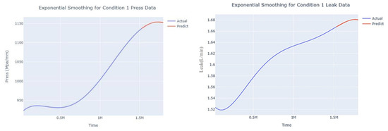
Figure 6.
Smoothed prediction diagram of pressure gain, leakage dynamic index for condition 1.
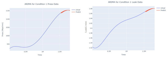
Figure 7.
Dynamic ARIMA prediction diagram of pressure gain, leakage for condition 1.
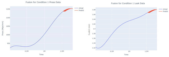
Figure 8.
Dynamic fusion prediction of pressure gain, leakage for condition 1.
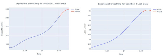
Figure 9.
Smoothed prediction diagram of pressure gain, leakage dynamic index for condition 2.
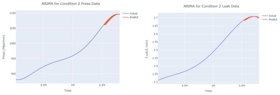
Figure 10.
Dynamic ARIMA prediction diagram of pressure gain, leakage for condition 2.
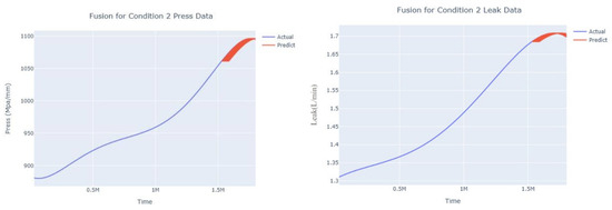
Figure 11.
Dynamic fusion prediction of pressure gain, leakage for condition 2.
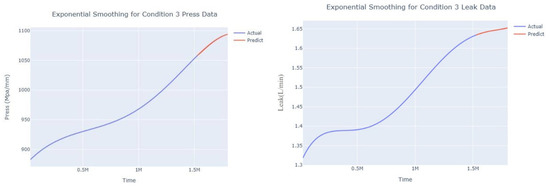
Figure 12.
Smoothed prediction diagram of pressure gain, leakage dynamic index for condition 3.
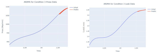
Figure 13.
Dynamic ARIMA prediction diagram of pressure gain, leakage for condition 3.
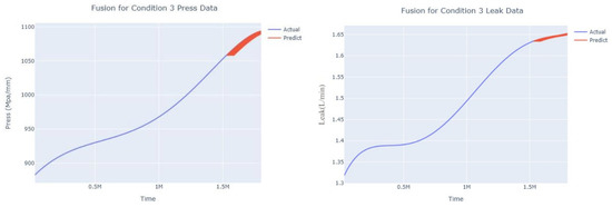
Figure 14.
Dynamic fusion prediction of pressure gain, leakage for condition 3.
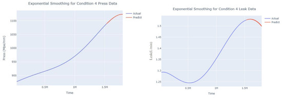
Figure 15.
Smoothed prediction diagram of pressure gain, leakage dynamic index for condition 4.
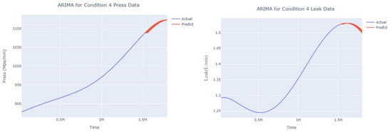
Figure 16.
Dynamic ARIMA prediction diagram of pressure gain, leakage for condition 4.
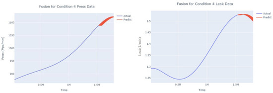
Figure 17.
Dynamic fusion prediction of pressure gain, leakage for condition 4.
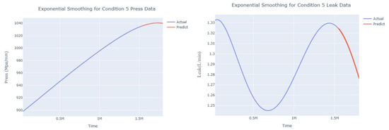
Figure 18.
Smoothed prediction diagram of pressure gain, leakage dynamic index for condition 5.
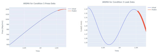
Figure 19.
Dynamic ARIMA prediction diagram of pressure gain, leakage for condition 5.
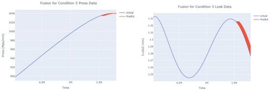
Figure 20.
Dynamic fusion prediction of pressure gain, leakage for condition 5.
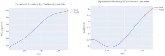
Figure 21.
Smoothed prediction diagram of pressure gain, leakage dynamic index for condition 6.
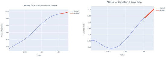
Figure 22.
Dynamic ARIMA prediction diagram of pressure gain, leakage for condition 6.
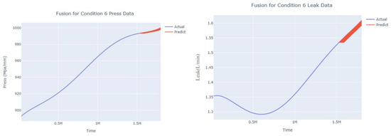
Figure 23.
Dynamic fusion prediction of pressure gain, leakage for condition 6.
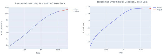
Figure 24.
Smoothed prediction diagram of pressure gain, leakage dynamic index for condition 7.
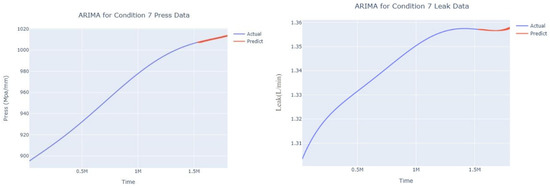
Figure 25.
Dynamic ARIMA prediction diagram of pressure gain, leakage for condition 7.
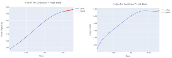
Figure 26.
Dynamic fusion prediction of pressure gain, leakage for condition 7.
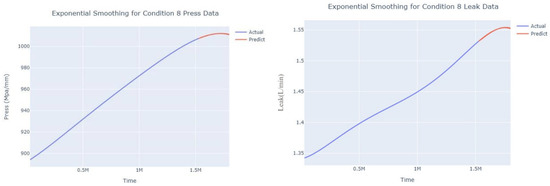
Figure 27.
Smoothed prediction diagram of pressure gain, leakage dynamic index for condition 8.
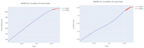
Figure 28.
Dynamic ARIMA prediction diagram of pressure gain, leakage for condition 8.
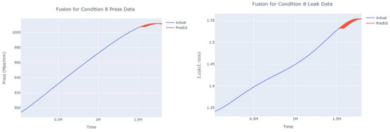
Figure 29.
Dynamic fusion prediction of pressure gain, leakage for condition 8.
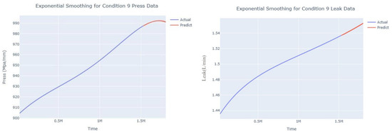
Figure 30.
Smoothed prediction diagram of pressure gain, leakage dynamic index for condition 9.
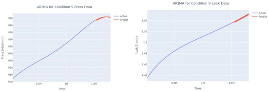
Figure 31.
Dynamic ARIMA prediction diagram of pressure gain, leakage for condition 9.
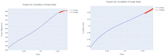
Figure 32.
Dynamic fusion prediction of pressure gain, leakage for condition 9.
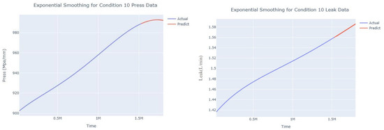
Figure 33.
Smoothed prediction diagram of pressure gain, leakage dynamic index for condition 10.
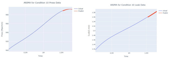
Figure 34.
Dynamic ARIMA prediction diagram of pressure gain, leakage for condition 10.
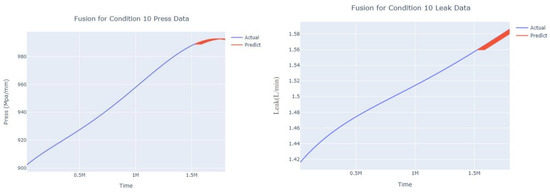
Figure 35.
Dynamic fusion prediction of pressure gain, leakage for condition 10.
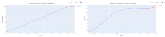
Figure 36.
Smoothed prediction diagram of pressure gain, leakage dynamic index for condition 11.
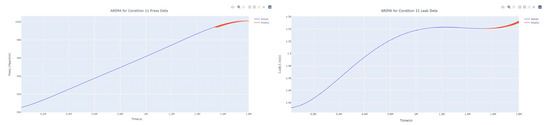
Figure 37.
Dynamic ARIMA prediction diagram of pressure gain, leakage for condition 11.
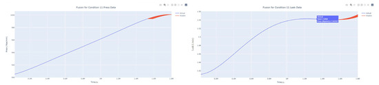
Figure 38.
Dynamic fusion prediction of pressure gain, leakage for condition 11.
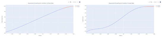
Figure 39.
Smoothed prediction diagram of pressure gain, leakage dynamic index for condition 12.
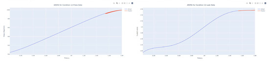
Figure 40.
Dynamic ARIMA prediction diagram of pressure gain, leakage for condition 12.
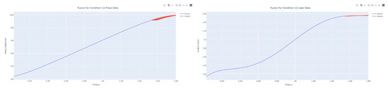
Figure 41.
Dynamic fusion prediction of pressure gain, leakage for condition 12.
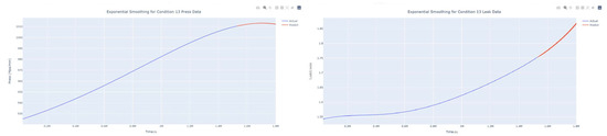
Figure 42.
Smoothed prediction diagram of pressure gain, leakage dynamic index for condition 13.
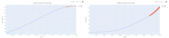
Figure 43.
Dynamic ARIMA prediction diagram of pressure gain, leakage for condition 13.
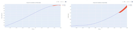
Figure 44.
Dynamic fusion prediction of pressure gain, leakage for condition 13.
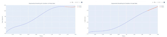
Figure 45.
Smoothed prediction diagram of pressure gain, leakage dynamic index for condition 14.
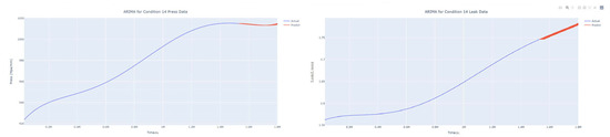
Figure 46.
Dynamic ARIMA prediction diagram of pressure gain, leakage for condition 14.
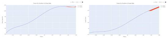
Figure 47.
Dynamic fusion prediction of pressure gain, leakage for condition 14.
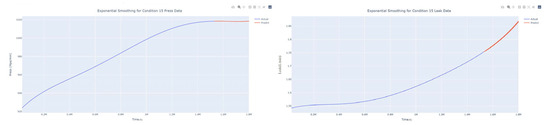
Figure 48.
Smoothed prediction diagram of pressure gain, leakage dynamic index for condition 15.
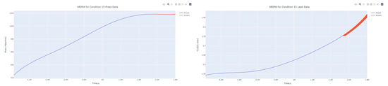
Figure 49.
Dynamic ARIMA prediction diagram of pressure gain, leakage for condition 15.
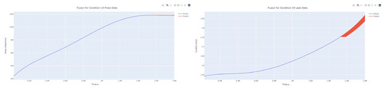
Figure 50.
Dynamic fusion prediction of pressure gain, leakage for condition 15.
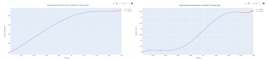
Figure 51.
Smoothed prediction diagram of pressure gain, leakage dynamic index for condition 16.
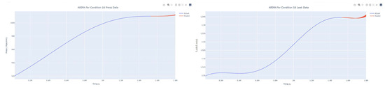
Figure 52.
Dynamic ARIMA prediction diagram of pressure gain, leakage for condition 16.
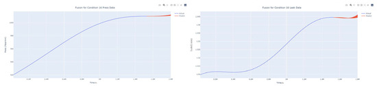
Figure 53.
Dynamic fusion prediction of pressure gain, leakage for condition 16.
Figure 6, Figure 7, Figure 8, Figure 9, Figure 10, Figure 11, Figure 12, Figure 13, Figure 14, Figure 15, Figure 16, Figure 17, Figure 18, Figure 19, Figure 20, Figure 21, Figure 22, Figure 23, Figure 24, Figure 25, Figure 26, Figure 27, Figure 28, Figure 29, Figure 30, Figure 31, Figure 32, Figure 33, Figure 34, Figure 35, Figure 36, Figure 37, Figure 38, Figure 39, Figure 40, Figure 41, Figure 42, Figure 43, Figure 44, Figure 45, Figure 46, Figure 47, Figure 48, Figure 49, Figure 50, Figure 51, Figure 52 and Figure 53 show that the exponential smoothing method predicted the best of the three prediction methods. Mean absolute error (MAE) and mean absolute percentage error (MAPE) are common measures of prediction accuracy in the process of optimizing the structural parameters of a neural network using an algorithm. MAE indicates the mean of the absolute value of the difference between the predicted and observed values, and MAPE indicates the mean of the absolute value of the difference between the predicted and observed values as a proportion of the observed values. The smaller the value of these indicators, the smaller the difference between the predicted and observed values, and the higher the prediction accuracy. In the process of using the algorithm to optimize the parameters, the MAE and MAPE indicators can be considered simultaneously to assess the prediction accuracy of the model in a comprehensive manner. The MAE and MAPE are calculated using the following formulae:
where is the mean value of the pressure gain and leakage samples, yi is the observed value at the ith operating time point, and is the predicted value at the ith operating time point.
The exponential smoothing method is better at predicting changes in performance indicators; for example, the mean absolute error (MAE) and mean absolute percentage error (MAPE) of pressure gain and leakage predicted dynamically using exponential smoothing 120 s in advance are shown in Table 3 and Table 4 below:
Table 3.
Prediction error statistics for pressure gain under exponential smoothing.
Table 4.
Prediction error statistics for leakage under the exponential smoothing method.
After the key performance indicators are predicted, life prediction can be made based on whether the failure threshold is reached. Because there is no international development and classification of failure standards for direct-drive electro-hydraulic servo valves or even other control valves, the research in this paper can only be based on the experience of the engineers of the institute that provides direct-drive electro-hydraulic servo valve samples and the requirements of the working environment restrictions in the aerospace industry, usually when the pressure gain is less than 2000 Mpa and the internal leakage is less than 2.5 L/min, wherein it can meet the aerospace servo Valve work requirements. The aim of this paper was therefore also to serve as a pre-requisite study and theoretical guide for the future development of servo valve failure standards in the aerospace sector. According to the long-term prediction results, the lifetime of the servo valve is about 1200 h or more, which is much higher than the 600 h required by the Chinese national standard [29].
4. Discussion
This paper implemented life prediction and reliability analysis of direct-drive electro-hydraulic servo valves through dynamic prediction of performance indicators. By monitoring and collecting data on the operating status of the servo valve, a large amount of performance index data, such as pressure gain and leakage, can be obtained. These data, combined with advanced machine learning and data analysis techniques, can establish a correlation model between servo valve performance indicators and life, and future life can be predicted and analyzed. The dynamic prediction results showed that the average absolute and average percentage error of this pressure gain and leakage was less than 0.05%, so all met the requirements of control areas such as industrial aerospace.
5. Conclusions
This paper used the application of exponential smoothing and the ARIMA algorithm to analyze and study the pressure gain (Mpa/mm), internal leakage (L/min), and other indicators of the slide-valve-type direct-drive electro-hydraulic servo valve, as well as carrying out the work of constructing a servo valve life prediction model based on the experimental data of the spool and sleeve of the slide-valve-type direct-drive electro-hydraulic servo valve in order to make predictions on the life of the slide-valve-type direct-drive electro-hydraulic servo valve The error analysis of the prediction results was carried out on the basis of the Copula function and the joint probability density distribution theory to verify the feasibility and universality of the algorithm used in this paper. It was also shown that the algorithm can be fully applied to the aerospace industry by using 16 sets of experimental data under the operating conditions of servo valves commonly used in the aerospace industry, and the prediction results indicated that this servo valve also met the life prediction requirements of the institute.
The research in this paper enables the pre-maintenance of servo valves, providing important references and guidance for engineering practice in related fields. The study also has a wide application prospect. It can be applied to various mechanical equipment’s life prediction and reliability analysis, providing technical support and guarantee for engineering practice and manufacturing.
Through the analysis and study of the experimental data, although the exponential smoothing method prediction theory, ARIMA, and other theories were discussed and models were constructed, the results needed to be more accurate. The causes of the problems were analyzed, and it was realized that the number and breadth of the samples selected were inadequate. In future research and optimization of direct-drive electro-hydraulic servo valves, a more comprehensive selection of pieces is needed, including the selection of models and categories for the whole range of servo valve applications to ensure a complete prediction theory of servo valve service life.
Author Contributions
G.H. proposed the research topic and direction, gave theoretical guidance, revised the paper, and provided some valuable suggestions; J.M. surveyed the literature and collected data, built the experimental bench and performed the experiments and data recording and processing, performed some simulations, analyzed the data, and then conceived and wrote the paper. All authors have read and agreed to the published version of the manuscript.
Funding
The authors would like to thank the National Key R&D Program of China (grant no. 2019YFB1703600) and the National Natural Science Foundation of China (grant no. 62033001).
Institutional Review Board Statement
Not applicable.
Informed Consent Statement
Not applicable.
Data Availability Statement
Data sharing is not applicable.
Conflicts of Interest
The authors declare no conflict of interest.
References
- Rodríguez-Martín, M.; Rodríguez-Gonzálvez, P.; Ruiz de Oña Crespo, E.; González-Aguilera, D. Validation of Portable Mobile Mapping System for Inspection Tasks in Thermal and Fluid–Mechanical Facilities. Remote Sens. 2019, 11, 2205. [Google Scholar] [CrossRef]
- Canales-Ide, F.; Zubelzu, S.; Segovia-Cardozo, D.; Rodríguez-Sinobas, L. Assessing the Performance of Irrigation Systems in Large Scale Urban Parks: Application to the Case of Valdebebas, Madrid (Spain). Remote Sens. 2022, 14, 1060. [Google Scholar] [CrossRef]
- Ni, T.-W.; Yang, Z.-G. Failure analysis on unexpected leakage of electro-hydraulic servo valve in digital electric hydraulic control system of 300 MW thermal power plant. Eng. Fail. Anal. 2020, 119, 104992. [Google Scholar] [CrossRef]
- Wang, S.-H.; Ni, T.-W.; Yang, Z.-G. Failure analysis on abnormal blockage of electro-hydraulic servo valve in digital electric hydraulic control system of 125 MW thermal power plant. Eng. Fail. Anal. 2021, 123, 105294. [Google Scholar] [CrossRef]
- Saha, B.K.; Peng, J.; Li, S. Numerical and Experimental Investigations of Cavitation Phenomena Inside the Pilot Stage of the Deflector Jet Servo-Valve. IEEE Access 2020, 8, 64238–64249. [Google Scholar] [CrossRef]
- Saha, B.K.; Li, S.; Lv, X. Analysis of pressure characteristics under laminar and turbulent flow states inside the pilot stage of a deflection flapper servo-valve: Mathematical modeling with CFD study and experimental validation. Chin. J. Aeronaut. 2020, 33, 1107–1118. [Google Scholar] [CrossRef]
- Shahkar, S.; Khorasani, K. A Multidimensional Bayesian Methodology for Diagnosis, Prognosis, and Health Monitoring of Electrohydraulic Servo Valves. IEEE Trans. Control Syst. Technol. 2022, 30, 931–943. [Google Scholar] [CrossRef]
- Yang, Y.-J.; Peng, W.; Meng, D.; Zhu, S.-P.; Huang, H.-Z. Reliability analysis of direct drive electrohydraulic servo valves based on a wear degradation process and individual differences. Proc. Inst. Mech. Eng. Part O J. Risk Reliab. 2014, 228, 621–630. [Google Scholar] [CrossRef]
- Rommel, D.; Di Maio, D.; Tinga, T. Calculating wind turbine component loads for improved life prediction. Renew. Energy 2020, 146, 223–241. [Google Scholar] [CrossRef]
- Aghajani, S.; Hemati, M.; Torabnia, S. Life prediction of wind turbine blades using multi-scale damage model. J. Reinf. Plast. Compos. 2021, 40, 644–653. [Google Scholar] [CrossRef]
- Thelen, A.; Li, M.; Hu, C.; Bekyarova, E.; Kalinin, S.; Sanghadasa, M. Augmented model-based framework for battery remaining useful life prediction. Appl. Energy 2022, 324, 119624. [Google Scholar] [CrossRef]
- Doremus, R.H. Life Prediction for Brittle Materials. Can. Met. Q. 2013, 23, 63–64. [Google Scholar] [CrossRef]
- Kong, Y.S.; Yu, J.; Park, Y.W. Creep Life Prediction of Alloy 718 for Automotive Engine Materials. Int. J. Automot. Technol. 2018, 19, 1055–1059. [Google Scholar] [CrossRef]
- Li, Y.; Wang, S.; Tomovic, M.M.; Zhang, C. Erosion degradation characteristics of a linear electro-hydrostatic actuator under a high-frequency turbulent flow field. Chin. J. Aeronaut. 2018, 31, 914–926. [Google Scholar] [CrossRef]
- Zhang, K.; Yao, J.; Jiang, T. Degradation assessment and life prediction of electro-hydraulic servo valve under erosion wear. Eng. Fail. Anal. 2014, 36, 284–300. [Google Scholar] [CrossRef]
- Seilsepour, H.; Zarastvand, M.; Talebitooti, R. Acoustic insulation characteristics of sandwich composite shell systems with double curvature: The effect of nature of viscoelastic core. J. Vib. Control 2023, 29, 1076–1090. [Google Scholar] [CrossRef]
- Talebitooti, R.; Gohari, H.; Zarastvand, M. Multi objective optimization of sound transmission across laminated composite cylindrical shell lined with porous core investigating Non-dominated Sorting Genetic Algorithm. Aerosp. Sci. Technol. 2017, 69, 269–280. [Google Scholar] [CrossRef]
- Liu, H.; Zhang, J.; Lu, C. Performance degradation prediction for a hydraulic servo system based on Elman network observer and GMM–SVR. Appl. Math. Model. 2015, 39, 5882–5895. [Google Scholar] [CrossRef]
- Yao, X.; Pecht, M. Performance Degradation of Hydraulic Vehicle Dampers. In Proceedings of the 2018 Prognostics and System Health Management Conference (PHM-Chongqing), Chongqing, China, 26–28 October 2018; pp. 364–368. [Google Scholar] [CrossRef]
- Siahpour, S.; Li, X.; Lee, J. A Novel Transfer Learning Approach in Remaining Useful Life Prediction for Incomplete Dataset. IEEE Trans. Instrum. Meas. 2022, 71, 1–11. [Google Scholar] [CrossRef]
- Wang, H.; Peng, M.-J.; Miao, Z.; Liu, Y.-K.; Ayodeji, A.; Hao, C. Remaining useful life prediction techniques for electric valves based on convolution auto encoder and long short term memory. ISA Trans. 2021, 108, 333–342. [Google Scholar] [CrossRef]
- Bhattacharya, S.; Maddikunta, P.K.R.; Meenakshisundaram, I.; Gadekallu, T.R.; Sharma, S.; Alkahtani, M.; Abidi, M.H. Deep Neural Networks Based Approach for Battery Life Prediction. Comput. Mater. Contin. 2021, 69, 2599–2615. [Google Scholar] [CrossRef]
- Ferreira, C.; Gonçalves, G. Remaining Useful Life prediction and challenges: A literature review on the use of Machine Learning Methods. J. Manuf. Syst. 2022, 63, 550–562. [Google Scholar] [CrossRef]
- Huang, G.; Mi, J.; Yang, C.; Yu, J. CFD-Based Physical Failure Modeling of Direct-Drive Electro-Hydraulic Servo Valve Spool and Sleeve. Sensors 2022, 22, 7559. [Google Scholar] [CrossRef] [PubMed]
- Lu, Y.-X. Hydraulic Pneumatic Technology Manual; Publishing Company of Machinery Industry: Beijing, China, 2002. (In Chinese) [Google Scholar]
- Jiang, X. Time Series Analysis and Prediction; Science Press: Beijing, China, 2018; p. 204. (In Chinese) [Google Scholar]
- Li, X. The COPULA Method and its Applications; Economic Management Press: Beijing, China, 2014. (In Chinese) [Google Scholar]
- GJB 420B-2015; Solid Particle Contamination Classes for Fluid of Aviation. AVIC Industrial Comprehensive Technology Research Institute: Beijing, China, 2015. (In Chinese)
- GJB 3370-1998; General Specification, Electrohydraulic Flow-Control Servovalves for Aircraft. AVIC Industrial Comprehensive Technology Research Institute: Beijing, China, 1998. (In Chinese)


Disclaimer/Publisher’s Note: The statements, opinions and data contained in all publications are solely those of the individual author(s) and contributor(s) and not of MDPI and/or the editor(s). MDPI and/or the editor(s) disclaim responsibility for any injury to people or property resulting from any ideas, methods, instructions or products referred to in the content. |
© 2023 by the authors. Licensee MDPI, Basel, Switzerland. This article is an open access article distributed under the terms and conditions of the Creative Commons Attribution (CC BY) license (https://creativecommons.org/licenses/by/4.0/).