Article

A Multivariate Machine Learning Model of Adsorptive Lindane Removal from Contaminated Water

by
Adeola Akeem Akinpelu
1,
Mazen K. Nazal
1,
Md Shafiullah
2,*,
Md Kamrul Islam
3,
Mohammed Monirul Islam
4,
Aminur Rahman
4,
Syed Masiur Rahman
1 and
Muhammad Muhitur Rahman
3,*
1
Applied Research Center for Environment & Marine Studies, King Fahd University of Petroleum & Minerals (KFUPM), Dhahran 31261, Saudi Arabia
2
Interdisciplinary Research Center for Renewable Energy and Power Systems, King Fahd University of Petroleum & Minerals, Dhahran 31261, Saudi Arabia
3
Department of Civil and Environmental Engineering, College of Engineering, King Faisal University, Al-Ahsa 31982, Saudi Arabia
4
Department of Biomedical Sciences, College of Clinical Pharmacy, King Faisal University, Al-Ahsa 31982, Saudi Arabia
*
Authors to whom correspondence should be addressed.
Appl. Sci. 2023, 13(12), 7086; https://doi.org/10.3390/app13127086
Submission received: 14 May 2023 / Revised: 3 June 2023 / Accepted: 12 June 2023 / Published: 13 June 2023
(This article belongs to the Section Environmental Sciences)

Abstract

:
It is challenging to use conventional one-variable-at-time (OVAT) batch experiments to evaluate multivariate/inter-parametric interactions between physico-chemical variables that contribute to the adsorptive removal of contaminants. Thus, chemometric prediction approaches for multivariate calibration and analysis reveal the impact of multi-parametric variation on the process of concern. Hence, we aim to develop an artificial neural network (ANN), and stepwise regression (SR) models for multivariate calibration and analysis utilizing OVAT data prepared through experimentation. After comparing the models’ performance, ANN was the superior model for this application in our work. The standard deviations (SD) between the observed and ANN-predicted values were very close. The average correlation coefficient (R2) between observed and ANN-predicted values for the training dataset was 96.9%. This confirms the ability of our developed ANN model to forecast lindane removal accurately. The testing dataset correlation coefficients (89.9% for ANN and 67.75% for SR) demonstrated a better correlation between observed and predicted ANN values. The ANN model training and testing dataset RMSE values were 1.482 and 2.402, lower than the SR values of 4.035 and 3.890. The MAPE values for the ANN model’s training and testing datasets, 0.018 and 0.031, were lower than those for the SR model. The training and testing datasets have low RSR and PBIAS values, implying model strength. The R2 and WIA values are above 0.90 for both datasets, proving the ANN model’s accuracy. Applying our developed ANN model will reduce the cost of removing inorganic and organic impurities, including lindane, and optimize chemical utilization.

1. Introduction

An organochlorine insecticide known as lindane (1r,2R,3S,4r,5R,6S-hexachlorocyclohexane, more commonly referred to as -HCH) has been the focus of extensive research in recent decades [1,2,3,4]. Since the 1940s, lindane has found widespread application in the fields of agricultural pest management, seed treatments, the treatment of poultry and cattle, domestic vector control, the protection of lumber, the treatment of lice and scabies, and even the treatment of rats using bait [5]. In soil, lindane is adsorbed to the soil particles, volatilized to the atmosphere, taken up by crop plants, or leached into groundwater. Even though lindane is treated, it still gets into creeks, rivers, lakes, and the ocean. Even a minimal amount of lindane in the water is dangerous. Lindane stays in the environment for a long time, where it can get into the cells of fish and, consequently, humans. Moreover, the pesticide may lessen the motility and concentration of sperm, alter the specific activity of a testicular marker enzyme, and cause oxidative stress in humans [6]. Additionally, it may cause testicular dysgenesis syndrome, alter serum testosterone levels, and reduce the amount of testosterone in the body. The presence of a significant number of chlorine atoms within the molecule of lindane causes it to be regarded as a substance that can cause disruptions to the body’s endocrine system [7]. This is because lindane is a highly toxic substance. Because of its high persistence level and ability to bioaccumulate and travel long distances, lindane is classified as a persistent organic pollutant, or POP [7]. As a result, there has been a rise in research focused on Lindane removal from contaminated water. The adsorptive removal method has been given a lot of preference in recent years because, compared to other ways, it has a very high efficiency at a low cost [8]. Adsorption, however, is controlled by several process variables, including temperature, pH of the medium, and contact time and concentration between the adsorbate and adsorbent. The impact of these parameters on the adsorption process is typically evaluated using batch adsorption studies that use the traditional OVAT approach [9]. This approach usually consumes time and resources and does not account for multivariate interactions among the variables [10]. Adsorption studies based on OVATs have challenges when examining multivariate/inter-parametric interactions between the physico-chemical parameters that synergize contaminant uptake [9]. Multivariate calibration and analysis using chemometric prediction techniques like ANN provide crucial insight into the impact of normative variability on the method in question [11].
The ANN is a tool that has recently become a powerful method for addressing issues prevalent in the real world and has garnered a great deal of attention due to its applications in various fields [12,13,14]. For example, it has been utilized in water treatment and offers solutions that are both practical and effective for the problem of water pollution [12]. However, the comparison of ANN and SR performances for the adsorption applications is scanty in the literature. In this work, however, we want to look at the model that will suggest optimum parameters that will give us the highest removal efficiency without rigorous experiments. These rigorous experiments consume a lot of time, energy, and cost. This is similar to the idea presented by Asadi et al. when they investigated multivariate optimization of mechanical and microstructural properties using AI tools [15].
Therefore, our interest in this work is to use the results from OVAT experiments to develop ANN and SR models that can be used for multivariate calibration and analysis. The performance of the two models was also compared, and it was confirmed that ANN was the best for this application. It is anticipated that the implementation of the developed ANN will result in a reduction of the overhead costs associated with the water treatment process. As a result of the application, the cost of removing numerous inorganic and organic pollutants in the contaminated water, such as lindane, will be reduced, and the usage of chemicals will be optimized.
The details of the developed models, adsorption experiment setup, and preliminary statistical details of the data set are described in the materials and method section of the manuscript. Subsequently, the strength of the developed predictive models based on the correlation coefficient values, root mean square error (RMSE), and mean absolute percentage error (MAPE) are compared and reported in the result section of the manuscript.

2. Materials and Methods

The proposed ANN’s theoretical foundation is presented in this section. In addition to the models and simulation data, the computational methods utilized to construct them are described.

2.1. Adsorption Experiment

Experiments with an OVAT were carried out at room temperature (24 °C) using the batch process method (Figure 1), and 25 mL of Deionized water with 5% methanol was used in the experiments. Lindane was added in varying concentrations to the solutions (0.05 to 2 mg L−1). The duration required to achieve equilibrium adsorption was ascertained by altering the shaking time at ambient temperature, utilizing a mass of 150 mg of adsorbent, and a rotational speed of 150 rpm, spanning a range of 5 to 5760 min. The effect of the amount of adsorbent was examined by manipulating the weight of the adsorbent within the range of 10 mg to 300 mg while keeping all other parameters unchanged. The impact of augmenting the primary Lindane level from 0.05 to 2 mg L−1 was examined similarly while keeping all other factors unchanged. Several standards and quality control samples were analyzed; some were blanks in which the adsorbent was present in the same solution without the adsorbate and others in which the adsorbate was present without the adsorbent. Using multiple reaction monitoring (MRM) modes on a GC-MS (GCMS TQ 8030 Shimadzu, Kyoto, Japan), we were able to calculate the concentrations of the analytes of interest. A 30 m 0.25 mm internal diameter Rxi-1 ms column with a 0.25 m film thickness was used (Restek, Bellefonte, PA, USA). The standard operating temperature for the instrument’s injector was 300 °C. Highly pure helium (99.999%) was used as the carrier gas, with a flow rate of 1.87 mL/min. An injection volume of 1.0 µL was performed in splitless mode. From 70 °C, the oven temperature was raised to 200 °C at 10 °C per minute. The detector was kept at a steady 250 °C.

2.2. Stepwise Linear Regression

Estimates of RA values were made using multiple stepwise regression (SR) in MATLAB (version 2019a). An onward and reverse selection was used in SR to zero in on the model’s most crucial parameters. The method was proposed to overcome problems with conventional multiple regression computation [16,17]. Multiple SR analysis has become a popular and helpful method in recent years. The technique is simple, flexible, and widely applicable [18]. SR is recommended for multiple independent variables [19]. The selection of SR was based on its capacity to handle many predictor factors, exhibit high computational efficiency, enable model fine-tuning, and facilitate prompt execution [20].
In SR, two stages are involved in determining the best possible set of predictors: Step-by-step reverse removal of insignificant parameters according to predetermined limit [21] and onward choice of input parameters in a “greedy style” to reduce the remainder of the squares at every stage. In this type of calculation, two distinct value thresholds are used for introducing and dropping parameters, respectively. If the importance of any potential parameters falls below a particular limit when an additional parameter is introduced to the set of factors that predict, SR will reject the new parameter. t-tests and F-tests are used in SR models to incorporate or eliminate variables that predict. The ideal combination of “N” predictor parameters is achieved in the final model. The Gauss–Jordan algorithm transforming rules, which consider the recurrent relationship among the regression coefficient, the remaining covariance variables, and the reverse of the covariance matrix’s partitioning elements, provide the conceptual foundation for a stepwise regression model. Assume mode begins with a forward choice with no variable that predicts (Equation (1)) to illustrate SR’s conceptual framework. Regression formulae can be completed by adding variables one at a time (Equation (2)) if they satisfy specific criteria (l F-ratio). To get rid of unnecessary predictors, sequential backward regression is performed.
y = β 0 + ε
y = β 0 + β 1 x 1 + β 2 x 2 + + β n x n + ε
In the current study, the independent variable is denoted by y, which represents the RA value. However, each of the dependent or explanatory variables, including retroreflective sheeting brand, grade, color, orientation, observation angle, age, and others, are represented by x1, x2, and xn. The regression coefficients, β0, β1, β2, and so on, estimate the relationship between the independent and dependent variables. Additionally, the random error is represented by ε.

2.3. Artificial Neural Networks

ANN is the most powerful computational technique for use in the fields of AI and ML right now. These computer programs, which take their cue from the individuals’ intellect, are meant to simulate learning by analyzing the physical principles and reasoning underlying challenging practical problems in the same way humans do [22]. The ANN’s construction, algorithm for processing, and ability to learn are all analogous to those of natural neurons in humans. Moreover, they are resilient to outside influences and can multitask, making them effective for detecting, classifying, grouping, and resolving prediction problems [23,24,25,26].
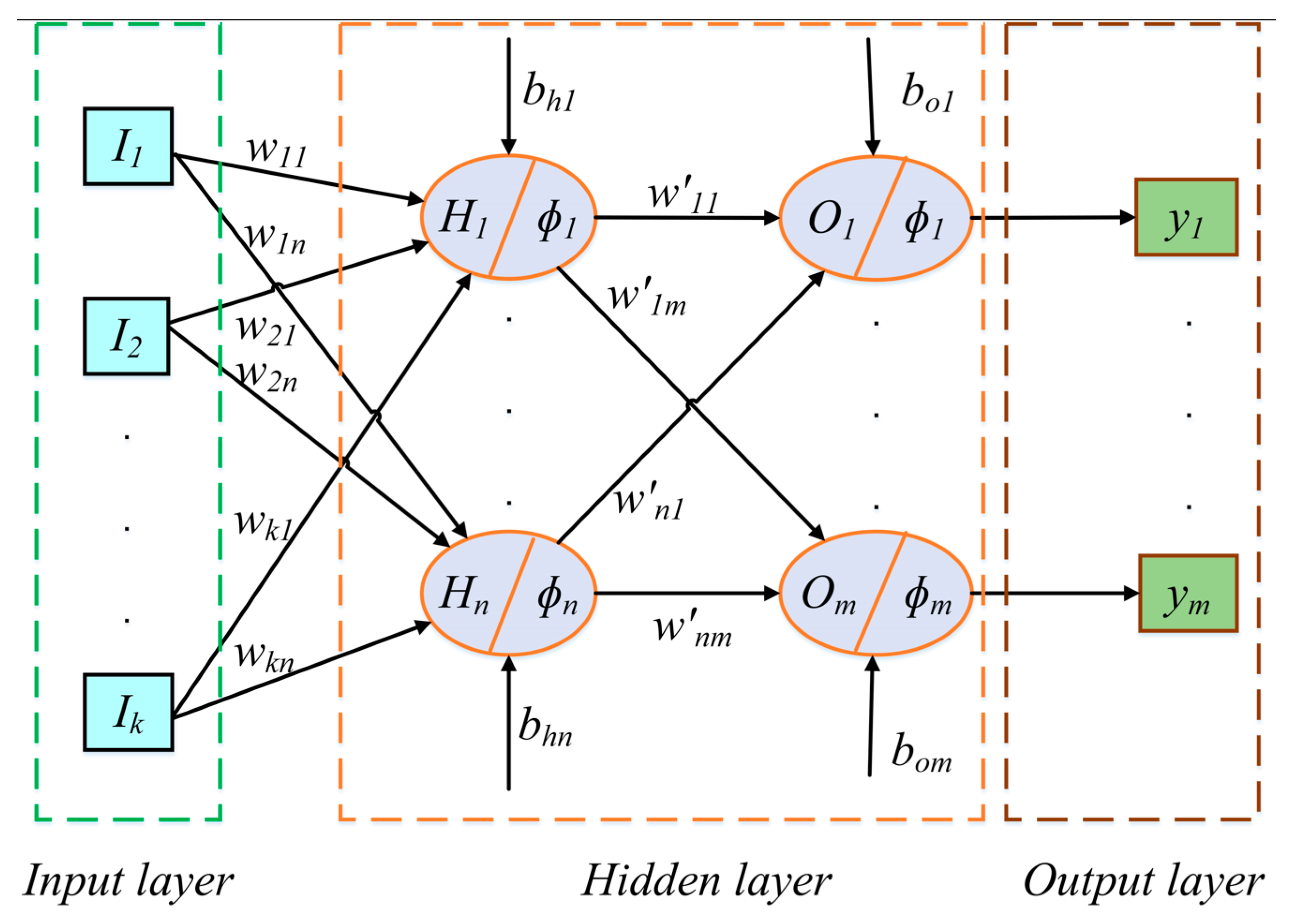
The multilayer perceptron (MLP) manifests a type of feedforward neural network (FFNN), the simplest kind of ANN. Models are built using controlled acquiring techniques in MLP neural networks (MLP-NN) by connecting input data to desired results. One or more “neurons,” or “cells,” can make up every “layer” of the neural processes. Weighted linkages relate the points in a specific layer to those in the following one. The data provided by each node are added together before being processed by a variety of nonlinear and biased functions. To pass on information to the following level of nodes, the result of every unit must be analyzed. This process is reiterated until reaching the output layer’s nodes [27,28,29].
Figure 2 depicts a simple MLP-NN design, which includes k inputs, n hidden nodes, and m outputs per hidden node. Ultimately, this MLP-NN produces m outputs from k inputs, one for each output node. The connection weights (wij) and biases (bij) of the MLP-NN are trained in two stages. To begin predicting outputs, inputs are “propagated” from the nodes that are concealed to the results of the nodes using arbitrary values and biases. The difference between the former and the latter is then determined. The MLP-NN then adjusts the biases and weights utilized in the relationships to minimize the value difference in the second stage. Lastly, it ceases revising the biases and weights after a certain period or if the gap between observed and predicted outputs remains constant [30,31].
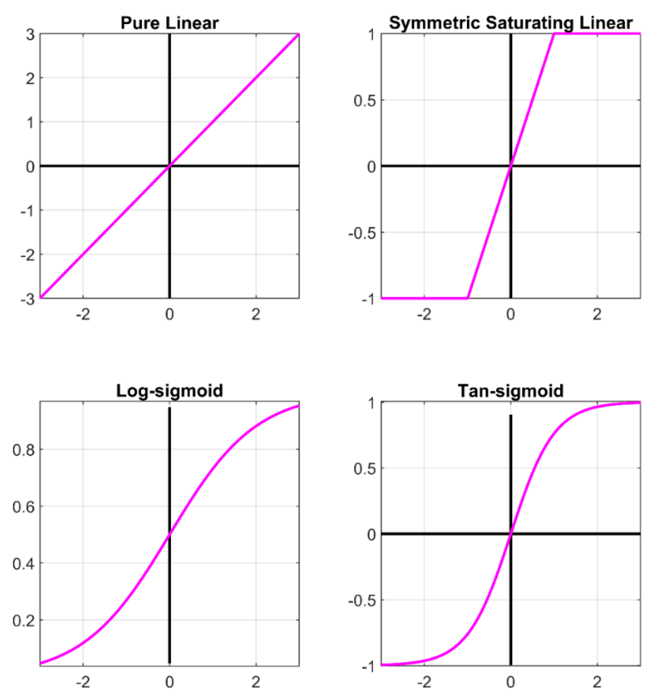
The relative strengths and weaknesses of the links among nodes are fine-tuned using a variety of methods of training in the neural system algorithm’s learning processes. Among the most popular methods are gradient descent (GD), resilient propagation (RP), Levenberg–Marquardt (LM), scaled conjugate gradient (SCG), and one-step secant propagation (OSS). Each method, as seen in [32], has advantages and disadvantages regarding precision, integration, pace, space requirements, and so on. Figure 3 [32] shows how artificial neural networks employ many different compressing or stimulating processes. A few examples include the linear, logistic sigmoid, softmax, tan sigmoid, and ReLU models.
The declining gradient issue, poor translation efficiency, overloading, and the necessity for repeated modification of the linking biases and weights are only a few of the problems plaguing traditional deep feedforward neural networks. This has led to studying numerous additional varieties of shallow neural networks [33,34,35]. Notable examples of such models are those based on a radial basis function (RBF), such as the extreme learning machine (ELM), the error correction model (EC), the improved second-order model (ISO), the K-nearest neighbor model (KNN), the logistic regression model (LR), the naïve Bayes model (NB), and the support vector machine (SVM).

2.4. Dataset Description

The proposed ANN model for predicting Lindane removal efficiency from contaminated water was developed from 49 datasets acquired from batch adsorption experiments. The effect of different parameters on the percentage removal of the lindane was investigated. The parameters are pH, initial concentration, temperature, contact time, and adsorbent dosage [36]. The experiments involve the adsorptive removal of lindane by seagrass powder from contaminated water. The computational tasks of the simulation and model-building processes presented in this research were performed utilizing the MATLAB computing environment. Before the developed model was put into use, the 49-dataset available for modeling was divided into two sets (training and testing sets), and 38 (77.5%) dataset was used as training. However, 22.5% of the data points (also known as the testing set) were used to test the model’s performance using three performance-measuring tools. The tools are correlation coefficient (R2), root mean square error (RMSE), and mean absolute percentage error (MAPE).
The input variables for the experiment are Dose (g), pH, Conc (mg/kg), Time (hrs), and Temp (C). However, we believe that the dataset used in this study has some limitations. The limitations involve the use of limited though common variables (5 parameters) as input to develop the models. Therefore, the model will only be valid to predict experiments that involve only these variables. Nevertheless, the limitations do not affect the performance of the model.
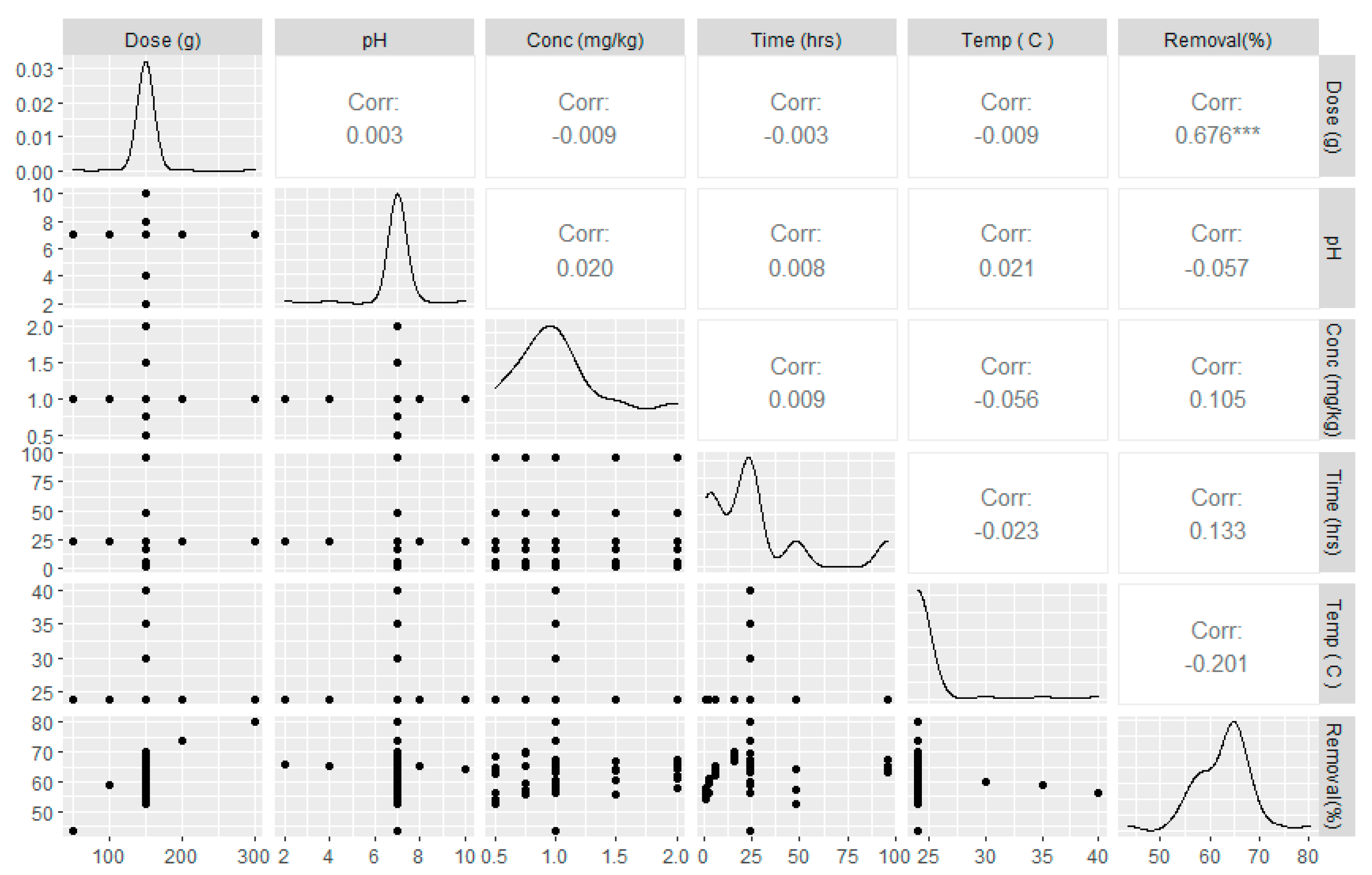
The data correlation matrix shows the associations between each pair of variables, and the result is presented in Figure 4. The correlation between any two input variables ranges from −0.201 to 0.676. These low values indicate that the input variables are unrelated.

2.5. Computational Methodology of the Developed Model

Selected Inputs (5): Dose (g), pH, Conc (mg/kg), Time (hrs), and Temp (C).
Selected Output (1): Removal (percentage).
FFNN: Activation function: tan-sigmoid, training algorithm: backpropagation (‘trainrp’); neurons in the hidden layer = 1 to 12 (4 neurons performed better than others); objective function: minimization of the MAPE of testing dataset. MATLAB function ‘newff’ was employed.
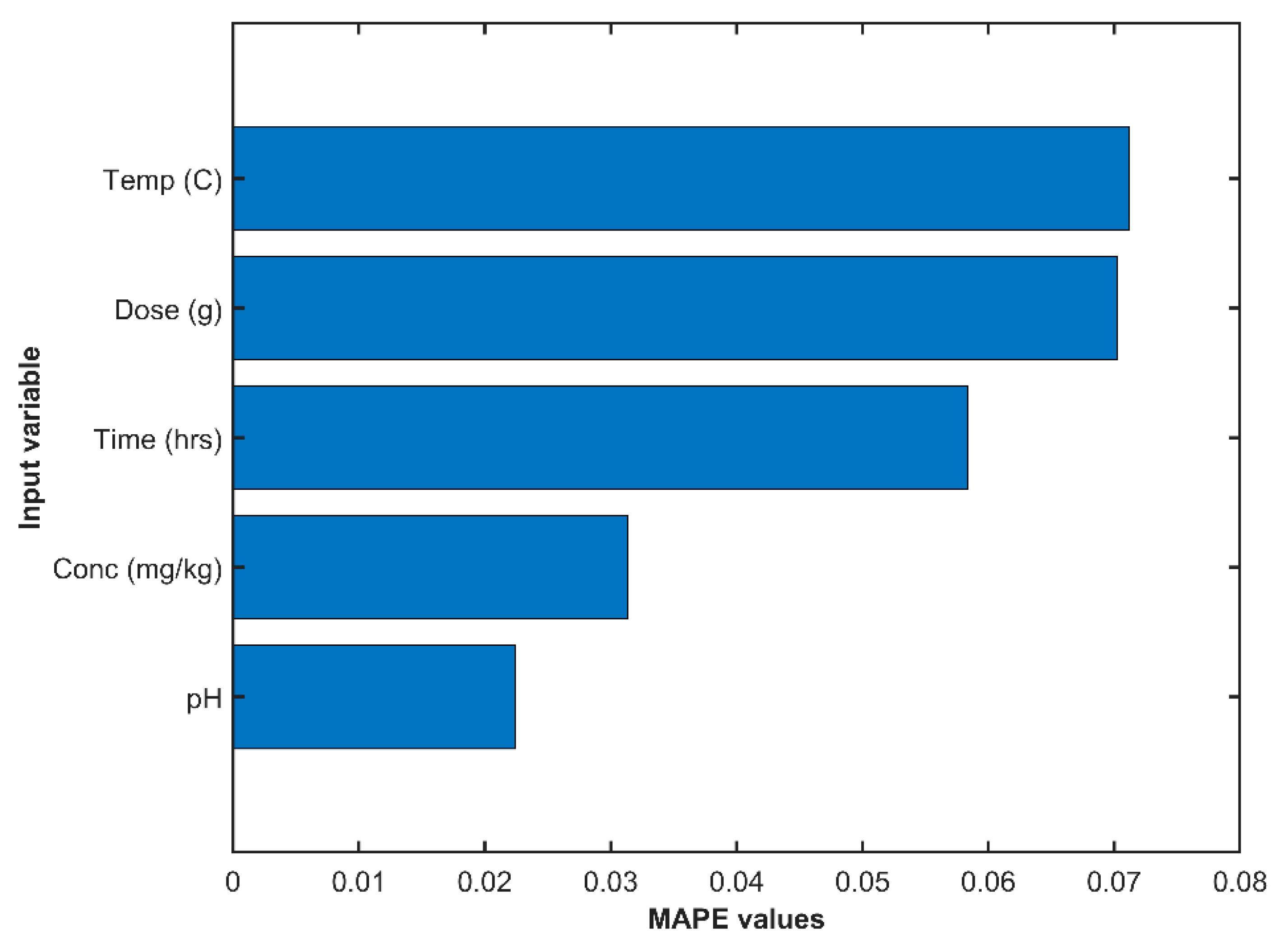
As reported in Table 1, the FFNNs were tested with four input variables by removing one input variable at a time for both data sets. The number of neurons in the hidden layers was kept fixed at 4. The MAPE values for each set of inputs were recorded. The higher MAPE values in the absence of a particular input variable referred to its higher importance in the input sets and vice versa, as can be seen from the following Figure 5.

3. Results and Discussion

Table 2 compares the predicted values of lindane removal efficiency under optimal conditions for each developed model with the experimentally measured values of lindane removal efficiency. The training records are between 1 and 38, and the remaining records were used for testing the model. The standard deviations (SD) were computed for each data set and applied to both the experimental and the predicted values. The ANN-predicted values were found to be much closer to the experimental values. There was very little difference between the two of them, which was mirrored by the fact that there was minimal variation in the ANN SD values [37].
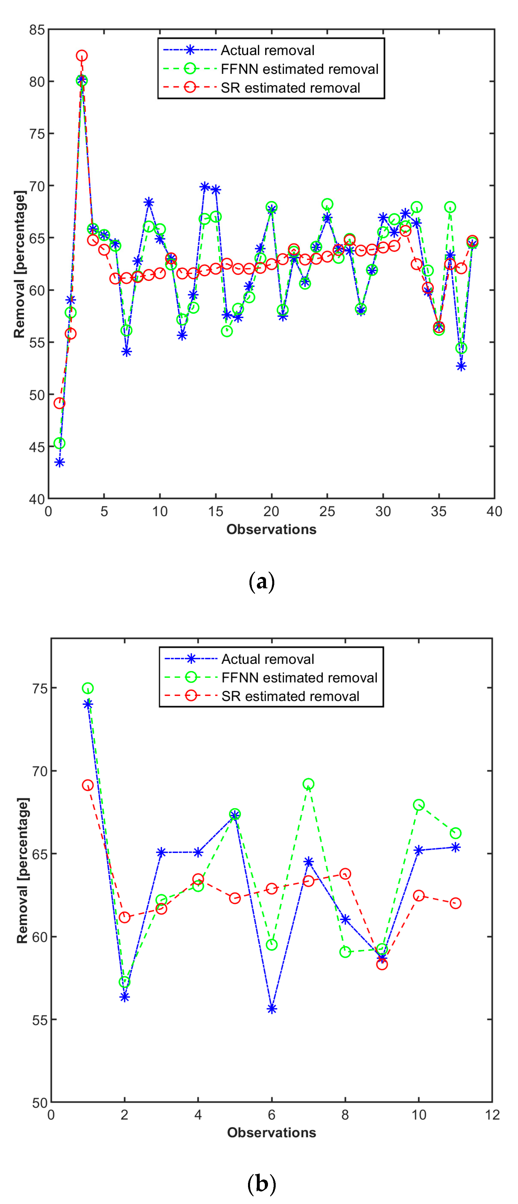
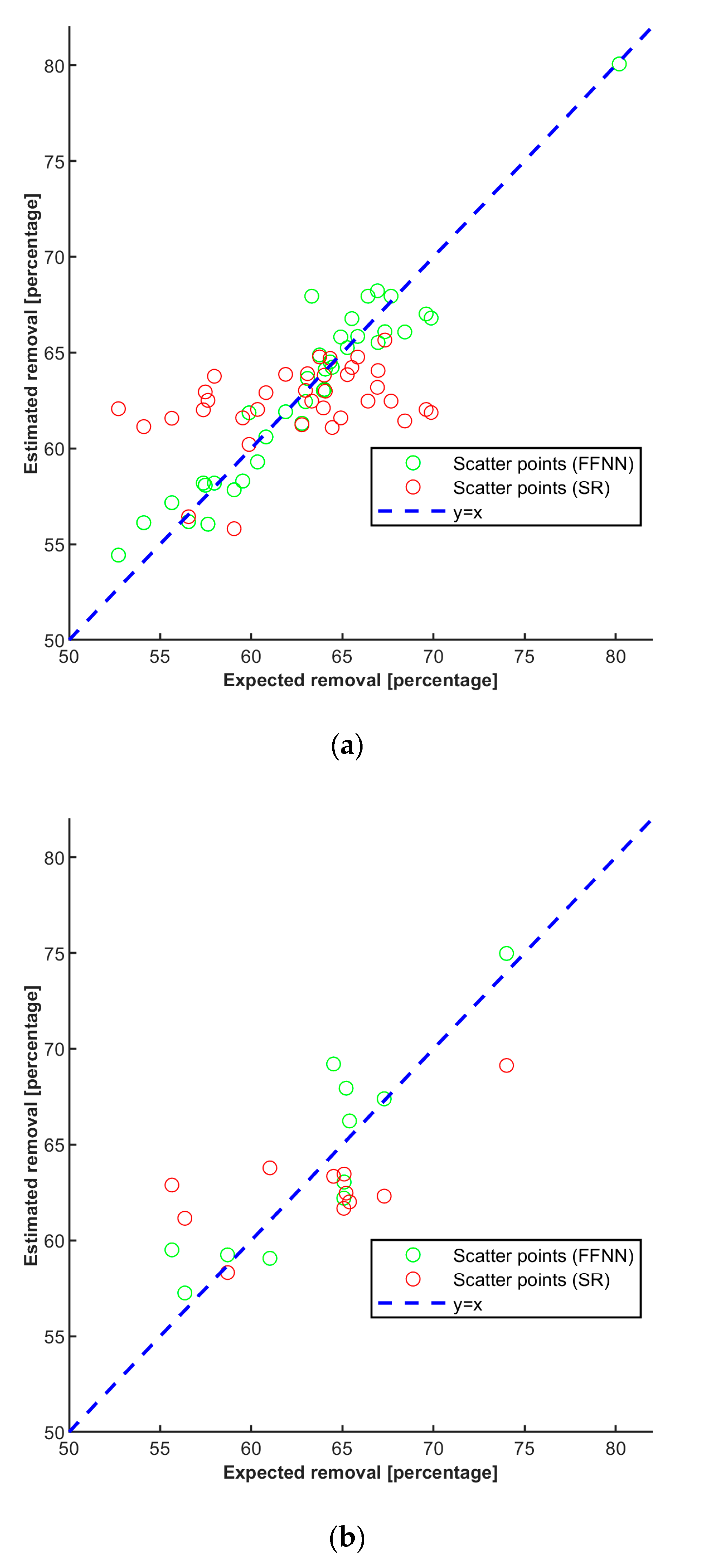
Therefore, it is evident in Table 2 that the developed ANN model performed better than the SR model for this application. Similarly, the results of the modeled and experimental values for the training dataset are displayed in Figure 6a. As the figure demonstrates, the ANN-predicted values coincided much better with the experimental values than the SR-predicted values. Overall, the correlation between the ANN-predicted and experimental values in most datasets shows that the model could accurately predict the experimental values. A linear curve was obtained when plotting the experimental data against the predicted values for the training dataset (Figure 7a) [38]. The average correlation coefficient (r) of the experimental and ANN predicted values were 96.9%, and of SR predicted value was 73.59%, which further confirms the power of our ANN model to predict removal efficiency values from experimental data accurately [39]. Previously, Tariq et al. reported similar performance when they used the ANN model for the adsorption of methylene blue on zeolite [40]. In the same vein, Figure 6b shows the experimental and predicted values results for the testing data set. The figure shows how well the experimental values and the ANN-predicted values agreed. To determine the degree of association or correlation coefficient between the two sets of values, the ANN and SR predicted values obtained from the developed models for the testing datasets were also plotted against experimental values (Figure 7b). The testing dataset obtained a correlation coefficient of 89.9% for ANN and 67.75% for SR, which showed a stronger association between the actual and ANN-predicted values.
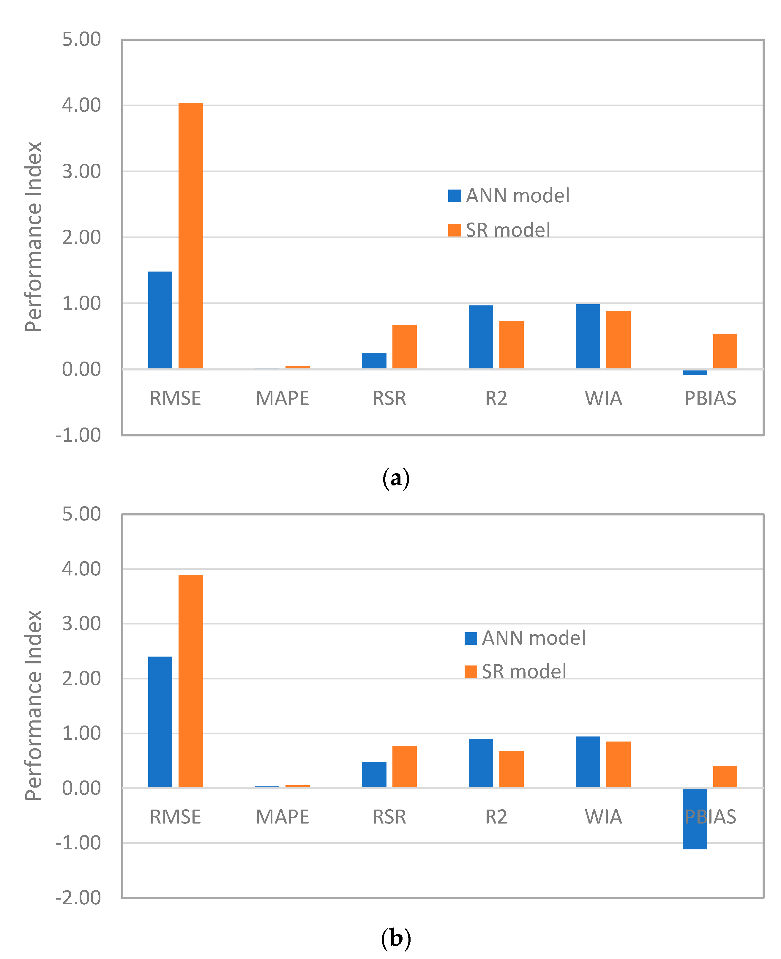
Additionally, RMSE, MAPE, and RSR are tools used to evaluate the error between the modeled values and experimental values. Lower RMSE, MAPE, and RSR values indicate a better model [41]. In contrast, the R2 and WIA values vary from ‘0’ to ‘1’, where the number ‘1’ indicates a perfect match between the actual and the estimated variables, whereas the number’ 0’ exhibits the output variables cannot be estimated from the given input variables. Besides, the ideal value of PBIAS is 0.0, which is a perfect match between the estimated and the actual variables. However, positive and negative values of PBIAS refer to underestimation and overestimation of the estimated outputs, respectively [42,43,44,45,46].
Table 3 presents the performance measuring parameters. RMSE, MAPE, and RSR represent a measure of the variances between values predicted by a model. The difference between experimental values and predicted values increases as the values rise. The ANN model’s RMSE values for the training and testing datasets were 1.482 and 2.402, respectively, which were significantly lower compared to the SR model’s RMSE values of 4.035 and 3.890 for training and testing, respectively. This was the conclusion of Altowayti et al. when they used ANN to study the adsorptive removal of arsenic [47]. Additionally, it was noted that the ANN model’s MAPE values for the training and testing datasets, which were 0.018 and 0.031, respectively, were significantly lower than the SR model’s MAPE values, as shown in Table 3 and presented in Figure 8. Likewise, the RSR and PBIAS values are low for both training and testing datasets, indicating the developed model’s strength. On the other hand, the R2 and WIA values are more than 0.90 for both datasets, which also testify to the efficacy of the developed ANN model. Furthermore, the equation generated from the developed ANN model will allow us to vary several parameters simultaneously, which was hitherto difficult with OVAT-based experiments [41]. Therefore, the multivariate/inter-parametric interactions between the physico-chemical factors that contribute to the adsorptive absorption of pollutants in a synergistic and non-interactive manner can be examined. As seen in Figure 8, the ANN model arguably demonstrates superior performance to the SR model across the board in terms of all of the performance measuring parameters considered in this study.

4. Conclusions

In this article, the ANN and SR models were proposed for multivariate calibration and analysis using the experimental data obtained from the OVAT experimentation. It was observed that the ANN was the better model for this application after comparing the performance of the two models. For each dataset, the standard deviations were calculated and applied to the experimental and the predicted values. The experimental and ANN-predicted values were discovered to be very close. A linear curve was produced when the experimental data were plotted against predicted values for the training dataset. The correlation coefficient, R2, between experimental and ANN predicted values was 96.9%, whereas the correlation coefficient between experimental and SR predicted values was 73.59% for the training dataset. This further supports the ability of our ANN model to predict lindane removal with accuracy. The computed correlation coefficients for the testing dataset—89.9% for ANN and 67.75% for SR—showed a stronger correlation between the actual and ANN predicted values. The RMSE values for the training and testing datasets for the ANN model were 1.482 and 2.402, respectively, which were noticeably lower than the corresponding SR model RMSE values of 4.035 and 3.890. It was also found that the MAPE values for the training and testing datasets for the ANN model, which were 0.018 and 0.031, respectively, were noticeably lower than those for the SR model. The RSR and PBIAS values, which represent the strength of the developed model, are also low for both the training and testing datasets. However, the R2 and WIA values are higher than 0.90 for both datasets, which further attests to the effectiveness of the developed ANN model. Therefore, it is believed that the overhead expenses related to the water treatment process are expected to decrease due to the application of our developed ANN model. The application will lower the cost of eliminating several inorganic and organic contaminants from the contaminated water, including lindane, and will optimize the use of chemicals.

Author Contributions

Conceptualization, A.A.A., M.S., M.K.N. and S.M.R.; methodology, M.K.N. and M.S.; software, M.S. and A.A.A.; formal analysis, M.S. and S.M.R.; resources, M.K.I. and M.M.I.; data curation, M.S. and M.M.R.; writing—original draft preparation, A.A.A., M.S. and M.M.R., writing—review and editing, M.M.R., A.R., M.K.N., S.M.R. and A.A.A.; supervision, M.K.N. and M.S.; project administration, M.S. and M.M.R.; funding acquisition, M.M.R. All authors have read and agreed to the published version of the manuscript.

Funding

This research was funded by the Deanship of Scientific Research at King Faisal University (KFU), Al-Ahsa 31982, Saudi Arabia, through Project No. GRANT 3415.

Institutional Review Board Statement

Not applicable.

Informed Consent Statement

Not applicable.

Data Availability Statement

The data that support the findings of this study are available from the corresponding authors, M.M.R. ([email protected]) and M.S. ([email protected]), upon reasonable request.

Acknowledgments

The authors acknowledge the support received from King Faisal University (KFU) and King Fahd University of Petroleum & Minerals (KFUPM), Saudi Arabia.

Conflicts of Interest

The authors declare no conflict of interest.

References

  1. Zhang, S.; Liu, Z.; Li, S.; Zhang, S.; Fu, H.; Tu, X.; Xu, W.; Shen, X.; Yan, K.; Gan, P.; et al. Remediation of Lindane Contaminated Soil by Fluidization-like Dielectric Barrier Discharge. J. Hazard. Mater. 2023, 443, 130164. [Google Scholar] [CrossRef] [PubMed]
  2. Yang, X.; Huang, X.; Cheng, J.; Cheng, Z.; Yang, Q.; Hu, L.; Xu, J.; He, Y. Diversity-Triggered Bottom-up Trophic Interactions Impair Key Soil Functions under Lindane Pollution Stress. Environ. Pollut. 2022, 314, 120293. [Google Scholar] [CrossRef] [PubMed]
  3. Pannu, R.; Kumar, D. Biodegradation of Lindane (γ-Hexachlorocyclohexane) and Other Isomers by Bacillus Subtilis Strain Mz-13i. Biocatal. Agric. Biotechnol. 2023, 48, 102630. [Google Scholar] [CrossRef]
  4. Khan, S.; He, X.; Khan, J.A.; Khan, H.M.; Boccelli, D.L.; Dionysiou, D.D. Kinetics and Mechanism of Sulfate Radical- and Hydroxyl Radical-Induced Degradation of Highly Chlorinated Pesticide Lindane in UV/Peroxymonosulfate System. Chem. Eng. J. 2017, 318, 135–142. [Google Scholar] [CrossRef]
  5. Vidal, J.; Carvela, M.; Saez, C.; Cañizares, P.; Navarro, V.; Salazar, R.; Rodrigo, M.A. Testing Different Strategies for the Remediation of Soils Polluted with Lindane. Chem. Eng. J. 2020, 381, 122674. [Google Scholar] [CrossRef]
  6. Pant, N.; Shukla, M.; Upadhyay, A.D.; Chaturvedi, P.K.; Saxena, D.K.; Gupta, Y.K. Association between Environmental Exposure to p, P′-DDE and Lindane and Semen Quality. Environ. Sci. Pollut. Res. 2014, 21, 11009–11016. [Google Scholar] [CrossRef]
  7. Raimondo, E.E.; Saez, J.M.; Aparicio, J.D.; Fuentes, M.S.; Benimeli, C.S. Bioremediation of Lindane-Contaminated Soils by Combining of Bioaugmentation and Biostimulation: Effective Scaling-up from Microcosms to Mesocosms. J. Environ. Manag. 2020, 276, 111309. [Google Scholar] [CrossRef]
  8. Akinpelu, A.A.; Nazal, M.K.; Abuzaid, N. Adsorptive Removal of Polycyclic Aromatic Hydrocarbons from Contaminated Water by Biomass from Dead Leaves of Halodule Uninervis: Kinetic and Thermodynamic Studies. Biomass Convers. Biorefin. 2021, in press. [Google Scholar] [CrossRef]
  9. Nath, B.K.; Chaliha, C.; Kalita, E. Iron Oxide Permeated Mesoporous Rice-Husk Nanobiochar (IPMN) Mediated Removal of Dissolved Arsenic (As): Chemometric Modelling and Adsorption Dynamics. J. Environ. Manag. 2019, 246, 397–409. [Google Scholar] [CrossRef]
  10. Akbari, M.; Asadi, P.; Aliha, M.R.M.; Berto, F. Modeling and Optimization of Process Parameters of the Piston Alloy-Based Composite Produced by Fsp Using Response Surface Methodology. Surf. Rev. Lett. 2023, 30, 2350041. [Google Scholar] [CrossRef]
  11. Asfaram, A.; Ghaedi, M.; Ghezelbash, R. Biosorption of Zn2+, Ni2+ and Co2+ from Water Samples onto Yarrowia Lipolytica ISF7 Using a Response Surface Methodology, and Analyzed by Inductively Coupled Plasma Optical Emission Spectrometry (ICP-OES). RSC Adv. 2016, 6, 23599–23610. [Google Scholar] [CrossRef]
  12. Alam, G.; Ihsanullah, I.; Naushad, M.; Sillanpää, M. Applications of Artificial Intelligence in Water Treatment for Optimization and Automation of Adsorption Processes: Recent Advances and Prospects. Chem. Eng. J. 2022, 427, 130011. [Google Scholar] [CrossRef]
  13. Shafiullah, M.; Abido, M.A.; Al-Mohammed, A.H. Intelligent Fault Diagnosis for Distribution Grid Considering Renewable Energy Intermittency. Neural Comput. Appl. 2022, 34, 16473–16492. [Google Scholar] [CrossRef]
  14. Ahmad, S.; Shafiullah, M.; Ahmed, C.B.; Alowaifeer, M. A Review of Microgrid Energy Management and Control Strategies. IEEE Access 2023, 11, 21729–21757. [Google Scholar] [CrossRef]
  15. Asadi, P.; Aliha, M.R.M.; Akbari, M.; Imani, D.M.; Berto, F. Multivariate Optimization of Mechanical and Microstructural Properties of Welded Joints by FSW Method. Eng. Fail. Anal. 2022, 140, 106528. [Google Scholar] [CrossRef]
  16. Breaux, H.J. On Stepwise Multiple Linear Regression; Army Ballistic Research Lab Aberdeen Proving Ground MD: Aberdeen, UK, 1967. [Google Scholar]
  17. Liu, W.-J.; Niu, X.-J.; Yang, N.; Tan, Y.-S.; Qiao, Y.; Liu, C.-F.; Wu, K.; Li, Q.-B.; Hu, Y. Prediction Model of Concrete Initial Setting Time Based on Stepwise Regression Analysis. Materials 2021, 14, 3201. [Google Scholar] [CrossRef]
  18. Wang, M.; Wright, J.; Brownlee, A.; Buswell, R. A Comparison of Approaches to Stepwise Regression on Variables Sensitivities in Building Simulation and Analysis. Energy Build. 2016, 127, 313–326. [Google Scholar] [CrossRef] [Green Version]
  19. Mundry, R.; Nunn, C.L. Stepwise Model Fitting and Statistical Inference: Turning Noise into Signal Pollution. Am. Nat. 2009, 173, 119–123. [Google Scholar] [CrossRef] [PubMed]
  20. Ali, Y.; Qin, A.; Aatif, H.M.; Ijaz, M.; Khan, A.A.; Ahmad, S.; Shahzad, U.; Yasin, M.; Rahman, S.U. A Stepwise Multiple Regression Model to Predict Fusarium Wilt in Lentil. Meteorol. Appl. 2022, 29, e2088. [Google Scholar] [CrossRef]
  21. Loftus, J.R.; Taylor, J.E. A Significance Test for Forward Stepwise Model Selection. Available online: https://arxiv.org/abs/1405.3920 (accessed on 13 April 2023).
  22. Krogh, A. What Are Artificial Neural Networks? Nat. Biotechnol. 2008, 26, 195–197. [Google Scholar] [CrossRef]
  23. Ali, A.; Almutairi, K.; Malik, M.Z.; Irshad, K.; Tirth, V.; Algarni, S.; Zahir, M.H.; Islam, S.; Shafiullah, M.; Shukla, N.K. Review of Online and Soft Computing Maximum Power Point Tracking Techniques under Non-Uniform Solar Irradiation Conditions. Energies 2020, 13, 3256. [Google Scholar] [CrossRef]
  24. Świetlicka, I.; Sujak, A.; Muszyński, S.; Świetlicki, M. The Application of Artificial Neural Networks to the Problem of Reservoir Classification and Land Use Determination on the Basis of Water Sediment Composition. Ecol. Indic. 2017, 72, 759–765. [Google Scholar] [CrossRef]
  25. Rahman, S.M.; Khondaker, A.N.; Hossain, M.I.; Shafiullah, M.; Hasan, M.A. Neurogenetic Modeling of Energy Demand in the United Arab Emirates, Saudi Arabia, and Qatar. Environ. Prog. Sustain. Energy 2017, 36, 1208–1216. [Google Scholar] [CrossRef]
  26. Ismail Hossain, M.; Shafiullah, M.; Abido, M. Induction Motor Speed Control Employing LM-NN Based Adaptive PI Controller. In Proceedings of the 18th International Conference on Renewable Energies and Power Quality (ICREPQ’20), Granada, Spain, 1–3 April 2020; Volume 18, pp. 97–102. [Google Scholar]
  27. Haykin, S. Neural Networks and Learning Machines, 3rd ed.; Pearson Education, Inc.: Upper Saddle River, NJ, USA, 2009. [Google Scholar]
  28. Aljohani, A.; Aljurbua, A.; Shafiullah, M.; Abido, M.A. Smart Fault Detection and Classification for Distribution Grid Hybridizing ST and MLP-NN. In Proceedings of the 2018 15th International Multi-Conference on Systems, Signals & Devices (SSD), Yasmine Hammamet, Tunisia, 19–22 March 2018; pp. 1–5. [Google Scholar]
  29. Shafiullah, M.; Abido, M.A. S-Transform Based FFNN Approach for Distribution Grids Fault Detection and Classification. IEEE Access 2018, 6, 8080–8088. [Google Scholar] [CrossRef]
  30. Tien Bui, D.; Tuan, T.A.; Klempe, H.; Pradhan, B.; Revhaug, I. Spatial Prediction Models for Shallow Landslide Hazards: A Comparative Assessment of the Efficacy of Support Vector Machines, Artificial Neural Networks, Kernel Logistic Regression, and Logistic Model Tree. Landslides 2016, 13, 361–378. [Google Scholar] [CrossRef]
  31. Rana, M.J.; Shahriar, M.S.; Shafiullah, M. Levenberg–Marquardt Neural Network to Estimate UPFC-Coordinated PSS Parameters to Enhance Power System Stability. Neural Comput. Appl. 2019, 31, 1237–1248. [Google Scholar] [CrossRef]
  32. Shafiullah, M.; Khan, M.A.M.; Ahmed, S.D. PQ Disturbance Detection and Classification Combining Advanced Signal Processing and Machine Learning Tools. In Power Quality in Modern Power Systems; Sanjeevikumar, P., Sharmeela, C., Holm-Nielsen, J.B., Sivaraman, P., Eds.; Academic Press: Cambridge, MA, USA, 2021; pp. 311–335. [Google Scholar]
  33. Huang, G.-B.; Zhou, H.; Ding, X.; Zhang, R. Extreme Learning Machine for Regression and Multiclass Classification. IEEE Trans. Syst. Man. Cybern. B Cybern. 2012, 42, 513–529. [Google Scholar] [CrossRef] [PubMed] [Green Version]
  34. Liu, H.; Lang, B. Machine Learning and Deep Learning Methods for Intrusion Detection Systems: A Survey. Appl. Sci. 2019, 9, 4396. [Google Scholar] [CrossRef] [Green Version]
  35. Cecati, C.; Kolbusz, J.; Rozycki, P.; Siano, P.; Wilamowski, B.M. A Novel RBF Training Algorithm for Short-Term Electric Load Forecasting and Comparative Studies. IEEE Trans. Ind. Electron. 2015, 62, 6519–6529. [Google Scholar] [CrossRef]
  36. Vinayagam, R.; Dave, N.; Varadavenkatesan, T.; Rajamohan, N.; Sillanpää, M.; Nadda, A.K.; Govarthanan, M.; Selvaraj, R. Artificial Neural Network and Statistical Modelling of Biosorptive Removal of Hexavalent Chromium Using Macroalgal Spent Biomass. Chemosphere 2022, 296, 133965. [Google Scholar] [CrossRef]
  37. Karaman, C.; Karaman, O.; Show, P.L.; Karimi-Maleh, H.; Zare, N. Congo Red Dye Removal from Aqueous Environment by Cationic Surfactant Modified-Biomass Derived Carbon: Equilibrium, Kinetic, and Thermodynamic Modeling, and Forecasting via Artificial Neural Network Approach. Chemosphere 2022, 290, 133346. [Google Scholar] [CrossRef]
  38. Gadekar, M.R.; Ahammed, M.M. Modelling Dye Removal by Adsorption onto Water Treatment Residuals Using Combined Response Surface Methodology-Artificial Neural Network Approach. J. Environ. Manag. 2019, 231, 241–248. [Google Scholar] [CrossRef]
  39. Sarafraz-Yazdi Ac, A.; Khaleghi-Miran, S.-H.; Es ’haghi Bc, Z. Comparative Study of Direct Immersion and Headspace Single Drop Microextraction Techniques for BTEX Determination in Water Samples Using GC-FID. Intern. J. Environ. Anal. Chem. 2010, 90, 14–15. [Google Scholar] [CrossRef]
  40. Tariq, R.; Abatal, M.; Bassam, A. Computational Intelligence for Empirical Modeling and Optimization of Methylene Blue Adsorption Phenomena Using Available Local Zeolites and Clay of Morocco. J. Clean. Prod. 2022, 370, 133517. [Google Scholar] [CrossRef]
  41. Igwegbe, C.A.; Mohmmadi, L.; Ahmadi, S.; Rahdar, A.; Khadkhodaiy, D.; Dehghani, R.; Rahdar, S. Modeling of Adsorption of Methylene Blue Dye on Ho-CaWO4 Nanoparticles Using Response Surface Methodology (RSM) and Artificial Neural Network (ANN) Techniques. MethodsX 2019, 6, 1779–1797. [Google Scholar] [CrossRef] [PubMed]
  42. Akinpelu, A.A.; Ali, M.E.; Owolabi, T.O.; Johan, M.R.; Saidur, R.; Olatunji, S.O.; Chowdbury, Z. A Support Vector Regression Model for the Prediction of Total Polyaromatic Hydrocarbons in Soil: An Artificial Intelligent System for Mapping Environmental Pollution. Neural Comput. Appl. 2020, 32, 14899–14908. [Google Scholar] [CrossRef]
  43. Lewis, C.D. Industrial and Business Forecasting Methods: A Practical Guide to Exponential Smoothing and Curve Fitting; Butterworth Scientific: San Diego, CA, USA, 1982; ISBN 0408005599. [Google Scholar]
  44. Shafiullah, M.; Abido, M.A.; Al-Mohammed, A.H. Power System Fault Diagnosis: A Wide Area Measurement Based Intelligent Approach, 1st ed.; Elsevier: Amsterdam, The Netherlands, 2022; ISBN 9780323884303. [Google Scholar]
  45. Moriasi, D.; Arnold, J.; Liew, M. Van Model Evaluation Guidelines for Systematic Quantification of Accuracy in Watershed Simulations. Trans. ASABE 2007, 50, 885–900. [Google Scholar] [CrossRef]
  46. Willmott, C.J.; Robeson, S.M.; Matsuura, K. A Refined Index of Model Performance. Int. J. Climatol. 2012, 32, 2088–2094. [Google Scholar] [CrossRef]
  47. Altowayti, W.A.H.; Algaifi, H.A.; Bakar, S.A.; Shahir, S. The Adsorptive Removal of as (III) Using Biomass of Arsenic Resistant Bacillus Thuringiensis Strain WS3: Characteristics and Modelling Studies. Ecotoxicol. Environ. Saf. 2019, 172, 176–185. [Google Scholar] [CrossRef]
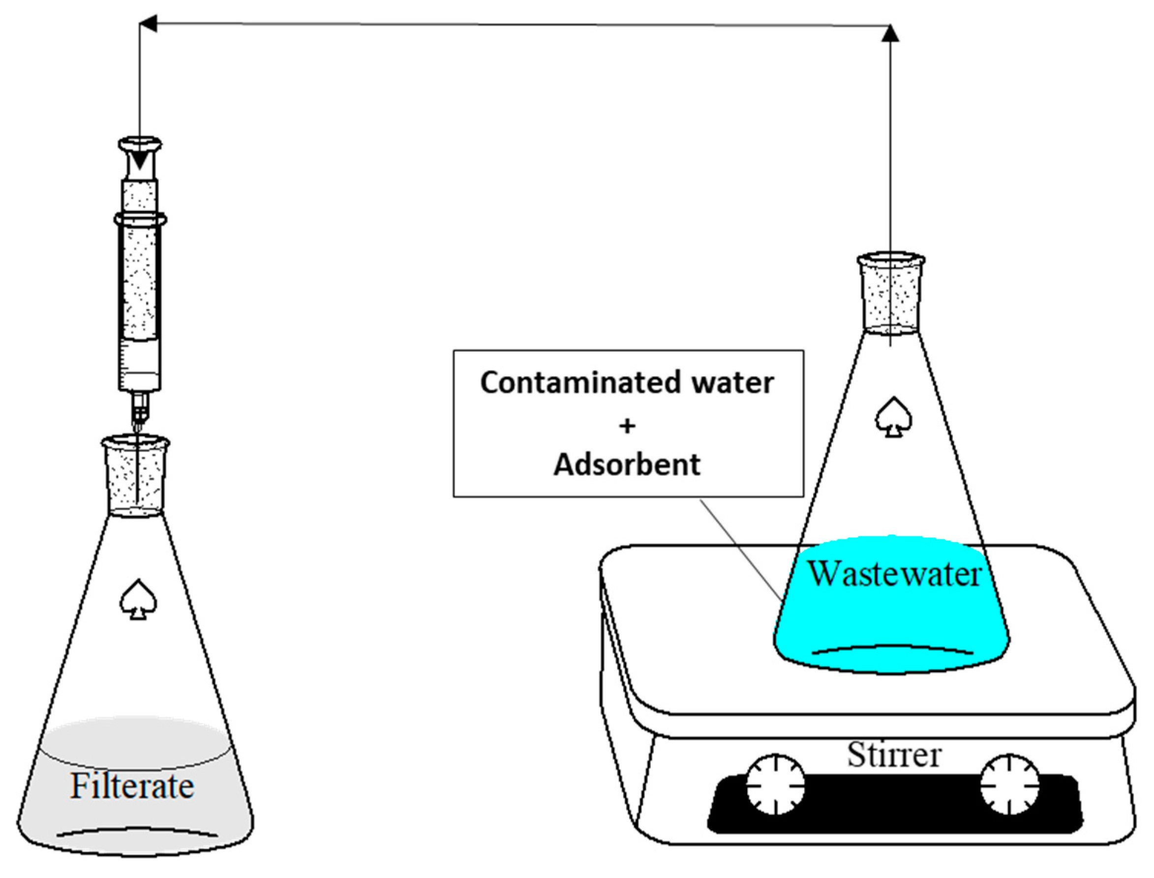
Figure 1. One-variable-at-time experimental setup.
Applsci 13 07086 g001
Figure 2. ANN model diagram.
Applsci 13 07086 g002
Figure 3. Squashing or activation functions.
Applsci 13 07086 g003
Figure 4. Statistical analysis of the raw dataset. *** symbolizes significance level at 0.01.
Applsci 13 07086 g004
Figure 5. MAPE Values for the Inputs.
Applsci 13 07086 g005
Figure 6. Line plots for the training dataset (a) and the testing dataset (b).
Applsci 13 07086 g006
Figure 7. Scatter plots for the training dataset (a) and the testing dataset (b).
Applsci 13 07086 g007
Figure 8. Performance measuring parameters for ANN and SR models for (a) Training dataset, (b) Testing dataset.
Applsci 13 07086 g008
Table 1. Minimization of MAPE.
Number of NeuronsMAPE
TrainingTesting
10.0525354680.051111675
20.0515373070.050463394
30.0481953530.050449361
40.0213378610.031621683
50.0238138190.048887605
60.0165720920.053637026
70.0161274810.036106327
80.016716850.046555818
90.0154280850.04684183
100.0103507450.050320977
110.0094772170.032474059
120.0111471930.034483183
Table 2. Experiment and predicted removal efficiency for all datasets with their standard deviation.
SNDose (g)pHConc (mg/kg)Time (hrs)Temp (C)Exp Values (%)ANN Predicted Values (%)LN Predicted Values (%)SD
ANN
SD
LN
15071242443.49245.31449.1451.2883.998
210071242459.05857.83755.8070.8642.299
330071242480.19480.06482.4550.0921.599
415021242465.83865.84664.7690.0060.756
515041242465.27265.25863.8490.0101.006
615071242463.31967.94462.4693.2710.601
7150101242464.44064.23361.0900.1462.369
815070.512454.10056.12261.1361.4304.975
915070.562462.77861.30661.2351.0411.091
1015070.5162468.42466.07761.4341.6604.943
1115070.5242464.91065.81561.5930.6402.346
1215070.5482452.71054.43062.0701.2176.618
1315070.5962462.97362.44463.0230.3740.036
1415070.7512455.63957.16761.5741.0814.197
1515070.7522459.52958.29661.5940.8721.460
1615070.75162469.86966.80361.8722.1685.655
1715070.75242469.59467.01862.0311.8215.348
1815070.75482457.62256.04562.5081.1153.455
191507112457.36858.19162.0120.5823.284
201507122460.34459.29762.0320.7401.194
211507162463.95463.02262.1120.6591.303
2215071242467.67067.94462.4690.1943.677
2315071482457.47558.07962.9460.4273.869
2415071962463.08563.65163.9000.4000.576
2515071.522460.80660.60062.9090.1461.487
2615071.562464.06464.13362.9880.0490.761
2715071.5162466.92268.22463.1870.9212.641
2815071.5482464.00663.07763.8230.6570.129
2915071.5962463.74564.87864.7770.8010.729
301507212457.97458.19063.7660.1524.095
311507262461.88461.91463.8650.0211.401
3215072162466.95565.52664.0641.0112.044
3315072242465.51966.77464.2230.8870.917
3415072482464.32664.51164.7000.1300.264
3515072962467.33166.09165.6530.8761.186
3615071242466.40467.94462.4691.0892.782
3715071243059.87961.85860.2071.3990.232
3815071244056.55856.17856.4350.2690.087
3915071242465.20667.94462.4691.9361.935
4020071242474.01074.97969.1310.6853.450
4115081242465.39266.23462.0090.5962.392
4215070.522456.35357.25661.1560.6393.396
4315070.7562465.07862.20661.6732.0312.407
4415070.75962465.09363.04563.4621.4481.154
4515071162467.29467.38962.3100.0673.524
4615071.512455.64559.50462.8892.7295.122
4715071.5242464.51469.20563.3463.3170.826
481507222461.02259.06663.7861.3831.954
4915071243558.69959.24758.3210.3870.267
Table 3. Performance measuring parameters.
ModelsClassRMSEMAPERSRR2WIAPBIAS
ANNTraining Data1.4820.0180.2490.9690.985−0.087
Testing Data2.4020.0310.4770.9000.943−1.113
SRTraining Data4.0350.0520.6770.7360.8850.541
Testing Data3.8910.0540.7720.6780.8510.404
Disclaimer/Publisher’s Note: The statements, opinions and data contained in all publications are solely those of the individual author(s) and contributor(s) and not of MDPI and/or the editor(s). MDPI and/or the editor(s) disclaim responsibility for any injury to people or property resulting from any ideas, methods, instructions or products referred to in the content.