Abstract
Water plays an important role in various physiological activities of living trees. Measuring trunk moisture content (MC) in real-time without damage has important guiding significance for transpiration research in forest ecosystems. However, existing standing tree MC detection methods are either too cumbersome to install or cause different degrees of damage. Here, we propose a novel Internet of Things (IoT) monitoring system that includes wireless acoustic emission sensor nodes (WASNs) and underground soil MC sensor nodes to efficiently detect and diagnose the MC level of living tree trunks. After the characteristic parameters were collected by the two sensors, a feature selection and multi-sensory global fusion method for MC diagnosis was designed and developed and several statistical parameters were selected as the input variables to predict the heartwood MC level with a support vector machine (SVM) model. Moreover, to achieve the highest prediction accuracy, an improved sparrow search algorithm (ISSA) is applied to ensure the most suitable parameter combinations in a two-objective optimization model. Extensive experiments result in a fusion of the environment, and AE signals show that the proposed mechanism has better diagnostic performance than state-of-the-art methods and is more adaptable to the fluctuation of working conditions.
1. Introduction
Forests are the largest ecosystem on Earth that human beings rely on for survival. They are also the most important barrier to protecting and ameliorating the ecological environment. In general, forests are made up of trees, shrubs, and herbs; the metabolism of forest plants depends on the orderly movement of water in their body [1]. In order to maintain normal growth, plants require a certain amount of water to support the conservation of energy in the ecosystem. However, for the interior water of plants, more is not always better [2,3,4]. Hence, the design and research of an effective and efficient real-time moisture content (MC) detection method for forest plants have drawn increasing attention recently, such as γ-ray [5], the resistance method [6], magnetic resonance imaging (MRI) [7], time domain reflectometry (TDR) [8], frequency domain capacitance (FD) [9], etc.
Among these existing methods, there are still some defects occurring unavoidably. The ray method has potential security risks; the resistance of the trunk is not intensely related to its moisture; MRI is an inconvenience in field application and is costly; TDR is a destructive testing method and is likely to cause considerable errors; and FD tends to be affected by the variation of trunk diameter [10]. Moreover, most of these achievements still follow manual or semi-automatic approaches, which poses an open challenge that should be tackled at full stretch to accomplish a fully autonomous forest monitoring system.
Meanwhile, the Internet of Things (IoT) is a very promising technology in the forestry engineering field, especially for the environment and plant growth monitoring [11,12,13], as shown in Figure 1. Among these, the wireless acoustic sensor network (WASN) has gained some particular insights into the wildlife recognition field [14,15]. It was deployed to monitor animal behavior in a non-intrusive manner by detecting and identifying different animal sounds. Additionally, the WASN has also been applied in wooden structural health monitoring, such as in our previous works [16]. It could capture the acoustic signal when wooden components suffer damage, and after data transmission, the sink would analyze and diagnose the details of the damage status.
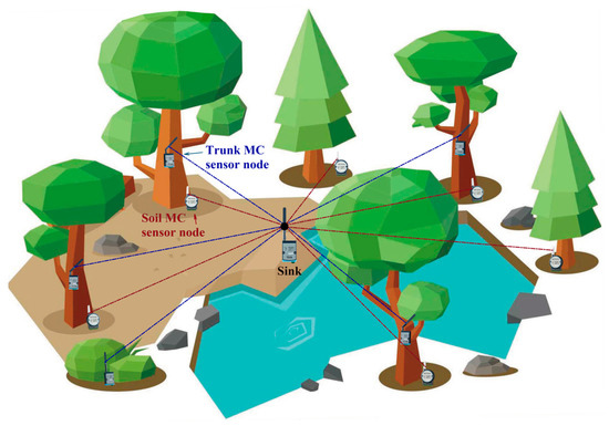
Figure 1.
The overall architecture of the forestry IoT for trunk MC monitoring.
Here, we intend to study a non-destructive WASN-based forest monitoring system to accurately detect the tree trunk’s MC level with convenience. This method mainly integrates the acoustic signal that is propagated along the tree bark, the soil humidity data, the ambient air temperature, and humidity data together to improve the measuring practicability and applicability. Additionally, an artificial intelligence technique is adopted to process the collected data and identify the MC level. In fact, recently, there are some references concerning the MC detection work on stones. Kai Tao et al. extracted six feature parameters from the original AE signals when compression tests were carried out on sandstone with different MC levels, and the identification of moisture was conducted using an SVM classifier [17]. Wei Zheng et al. measured the effect of moisture on the AE characteristics of rocks and established a musical-staff-inspired MC detection model [18]. In [19], an AE multi-parameter analysis for dry and saturated sandstone with cracks under uniaxial compression was presented. Furthermore, soil physical characterization has employed AE tools as well; M. NaderiBoldaji et al. developed a new soil multi-sensor fusion by combining mechanical, dielectric, and acoustic responses in layered soils for the estimation of soil water content, degree of compactness, and texture [20]. Tate designed a vertical cone penetrometer with an acoustic sensor to correlate the acoustic signal with soil moisture [21]. As for timber detection, the AE technique certainly has many applications [22], whereas, for the MC measurement of woody plants, only a few studies have been introduced. Linus De Roo et al. studied the use of AE for the detection of trees’ vulnerability to drought [23]. Bert Peeters et al. reviewed the status of cavitation-related AE [24]. Kensuke Kageyama et al. found that the AE behaviors of Schefflera and Olive trees were strongly influenced by drought stress [25].
Most of the above pieces of literature show the sophisticated and specialized utilization of the AE signal. One single type of sensor is limited in acquiring all the necessary signals that reflect the MC level of plants due to the interference of complex operating conditions, especially when considering the anisotropy of tree trunks [26]. Thus, multi-sensory fusion is essential for a comprehensive and high-reliability measuring system. Therefore, in this research, we propose a multi-sensor data fusion method for MC detection while processing the AE, temperature, and humidity data from a WASN-based forestry IoT. We have deployed the WASN and wireless underground soil MC sensor nodes in a sample forest, and different feature parameters have been collected to carry out the intensive study. Our contributions can be summarized as follows:
- (1)
- We analyzed the AE signals propagated along the surface of tree bark under different MC levels. Signal processing is conducted to extract different AE features for classification purposes.
- (2)
- The Maximum Correlation and Minimum Redundancy (mRMR) algorithm is used to screen out the optimal feature subset related to the MC condition of a standing tree trunk, and then data fusion is performed based on a conditional information entropy weight mechanism. After that, an SVM model is adopted to diagnose the MC status, and a firefly disturbance strategy is used to improve its global searching ability. So, the hyper-parameters have been optimized by this improved sparrow search algorithm (ISSA).
- (3)
- With data fusion of the multi-sensors, the degree of MC levels could be accurately predicted with an error noticeably lower than the AE sensors alone.
- (4)
- We perform comprehensive experiments to examine the feasibility and capability of the proposed tree trunk MC detection system, and results show that it exhibits excellent performance in field-testing and is superior to the traditional methods in long-term measurement.
2. Materials and Methods
2.1. Wireless Acoustic Emission Sensor Network
Generally, the proposed WASN is an extension of the WSN equipped with AE sensors. This specified wireless AE node is capable of managing up to two independent AE channels, and each channel is provided with a low-noise high-speed amplifier OPA627 [27]. In addition, the conditioned AE channels are connected to a 12-bit low-power analog-to-digital converter AD7356 [28] with a fixed sampling frequency of 5 MHz. Then, an ARM Cortex-M4 micro-controller STM32F405RG [29] under 168 MHz would take charge of the whole data flow and finally, a LoRa® module SX1278 [30] would be adopted for the wireless communication assignment. The composition structure of the AE node and its application architecture are shown in Figure 2.
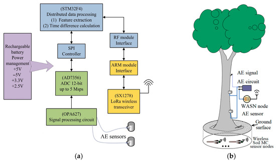
Figure 2.
Structure and installation of system: (a) architecture of the wireless AE node; (b) diagram of system installation.
The AE signal is generated by one mini vibration motor based on Arduino that has been mounted closely on the trunk [31]. The stress wave generated during the test would propagate through the tree trunk surface and be collected by the AE sensors attached to the bark. In order to enhance the anti-interference ability of the AE system, two R15α type probes are vertically placed around the diameter of the breast height (DBH) of trees (1.3 m above the ground) with an interval of 10 cm, according to Kexiang Li’s research [32]. The AE signal source is placed vertically on the upper side of the two probes 10 cm away from the near-end probe, all within a three-point line. This means that the differential term of AE signals between the far-/near-end probes can be calculated to reduce the system measuring error as much as possible. The WASN has been deployed at the sample woods of an experimental forestry farm in Nanjing Forestry University, China. A remotely deployed sink that aggregates all the nodes’ feature data would take charge of the next dataset’s analyzing and processing procedure.
2.2. Environmental Parameter Monitoring IoT
The environmental monitoring IoT system has the capability to capture surrounding forestry growth information by using an Arduino-compatible board along with a LoRa® transmitter. The collected information includes light intensity, temperature and humidity at DBH, and underground soil humidity data at two depths (10 cm and 20 cm). Reference [33] indicated that the MC level of a single tree trunk is closely related to the soil humidity value within 20 cm below the surface. Note that the temperature and humidity sensors only consider snapshot data every 45 min due to their slow variation. The extra-large-volume alkaline battery is installed and is able to supply power to each sensor node effectively and efficiently. The practical prototypes of the WASN and wireless soil nodes are shown in Figure 3.
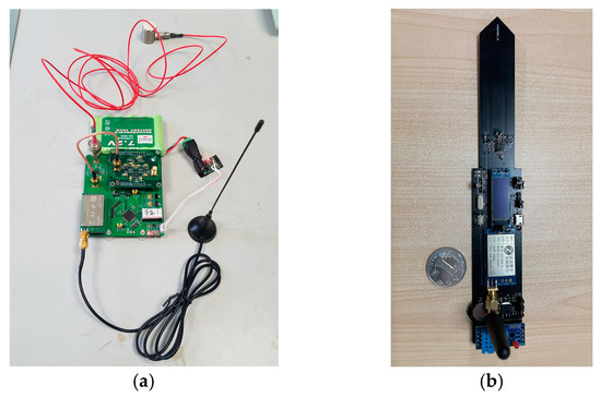
Figure 3.
The prototype of designed wireless sensor nodes: (a) architecture of the wireless AE node; (b) architecture of the soil moisture sensor.
2.3. System Architecture
The proposed multi-sensory MC detection system follows a centralized architecture where the diagnosis process takes place in the gateway. This allows us to implement lightweight nodes for the distributed independent signal processing units. The simplification in the nodes could reduce their costs and energy consumption drastically, which are the main constraints for WASN deployment in the field.
The whole system structure diagram is depicted in Figure 4. It contains three main elements: (1) the wireless nodes, which are in charge of sensing the AE signals and environmental parameters, along with transmitting the featured data to the sink through wireless communication; (2) the gateway, which has a strong computational ability and is able to coordinate the whole wireless network and gather all the sensor nodes’ data; and (3) the diagnostic program, which provides the intelligent learning functionality through the fusion of the AE signal and environment parameters’ individual scores.
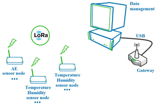
Figure 4.
The proposed monitoring system’s organizational structure.
2.4. Diagnosis Methodology
The proposed data processing and diagnosis mechanism aims to detect the heartwood MC level non-destructively at the point of measurement under the AE signal and environment parameters. Thus, to design the diagnosis methodology, tests over different types of tree trunks have been carried out by means of specific laboratory MC measuring instruments. The objective is to characterize the relationship among the AE signal feature, environmental temperature, and humidity data under different MC levels. The whole detection operates in the following two processes:
- (1)
- Training process: In this stage, we first build up a dataset containing both AE and environment parameters, which are induced by the MC variations for 12 months. Note that target trees are required to distribute a safe circumstance for obtaining reliable features. Then, we select the optimal AE features and environmental data under the greatest correlation with the MC level by utilizing a dimension reduction algorithm as the next training input for ease of maximizing the expression from original data information and improving the hardware calculation efficiency. Afterward, a delicately designed machine-learning algorithm is adopted to fit the characteristics of sampled data, which would continuously vary with time. Finally, this diagnostic model should be carried out to detect the living tree heartwood’s MC level.
- (2)
- Detection process: In this stage, we estimate the MC level of field woods based on the aforementioned achievement. Acquired parameters will be pre-processed and normalized. Next, it is input into an adaptive dynamic weighting module to calculate the individual influence of each feature on the MC level. Then, we combine the results in a weight fusion algorithm and finally predict the testing trunk’s MC. The overview of the diagnostic system is shown in Figure 5.
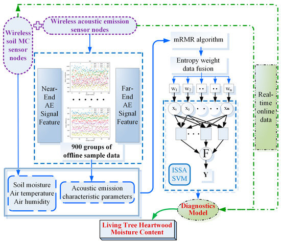 Figure 5. Diagram of the proposed MC diagnostic method.
2.5. Data Processing
By collecting the AE characteristic parameters on the bark, soil MC value around standing trees’ roots, air humidity, and temperature information at DBH as a whole sample dataset, the MC level of the living tree heartwood can be detected by an intelligent multi-sensor data fusion algorithm. The main idea is to first adopt the mRMR algorithm for an optimal feature dimension reduction. Next, the selected feature would be fused by using the conditional entropy weight method. Then, the enhanced SVM model is used to establish an offline diagnosis system, and the ISSA is employed to optimize the operational parameters, which further improves the model’s generalization ability and overcomes the overfitting issue. Finally, the devised model is applied to the online long-term multi-sensory MC prediction adaptively and efficiently.
2.5.1. Maximum Correlation and Minimum Redundancy Algorithm
The mRMR algorithm is a feature selection method that maximizes the correlation between feature variables and targets and minimizes the correlation between features. Mutual information is used as the standard to measure the correlation between features and category variables:
where I(x;y) is the mutual information between the feature variables x and y, and their probability densities and joint probability densities are p(x), p(y), and p(x,y), respectively.
In order to find the feature subset S which contains the optimal m features, the maximum correlation principle takes I(xi;c) to search for the m features related to target category c in the appropriate order, which can be measured and calculated by the following formula:
However, the subset with m features may not necessarily be the perfect feature subset. In particular, if there are two features that are interdependent, the minimum redundancy criterion should be introduced to eliminate them by using Equation (3); then, the operator Φ could be used to integrate the maximum correlation coefficient and minimum redundancy by using Equation (4).
Thus, the ranking of each feature variable in the sample set S can be calculated. In this paper, the time domain parameters of near/far-end AE signals are chosen as the feature vectors, as they have a relatively fast diagnostic speed and a fairly high detection accuracy. After data normalization, mRMR could just be operated for feature dimension reduction.
2.5.2. Data Fusion Based on Conditional Information Entropy Weight Allocation
In the process of multi-sensor information fusion, different sensor data represent different attributes, and the importance of different attributes should be considered before fusion. To some extent, the weight of the data reflects the influence of attributes on the final prediction results; the greater the weight, the greater the influence. The target at the weight allocation of different sensor data and the change in information entropy, after taking data into account when making decisions, was analyzed according to the information entropy theory to realize an information-gain-based data weight allocation. In addition, the following formula is used to calculate information entropy:
In this formula, Pi represents the corresponding decision probability of corresponding attribute data. In the process of weight allocation, the decision probability without considering attribute data is calculated first, and the original information entropy is obtained. Next was the information entropy after adding attribute data, namely conditional information entropy. According to the difference between original information entropy and conditional information entropy, the higher the information entropy, the greater the influence of attribute data on decision-making and the greater the fusion weight allocated.
Let the optimized feature parameter obtained by mRMR be x1, x2, and …, xn, and let the decision variable be I. Then, the process of feature weighting should be calculated as follows:
- (1)
- Calculation of the original information entropy H(I):
SS(I) stands for the state space of decision variable I.
- (2)
- Calculation of correspondingly conditional information entropy H(I|), H(I|), …, and H(I|) after taking different attribute data into account, when ::
- (3)
- Calculation of the difference value between the conditional and original information entropy Δ(I, x1), Δ(I, x2), …, Δ(I, xn) with the following formula:
- (4)
- Calculation of different attribute data’s weight vectors according to the difference value of information entropy:
2.5.3. Support Vector Machine Method
The SVM is a machine learning method based on statistics theory, which has an excellent performance in dealing with nonlinear problems with small samples and high dimensions. The purpose of the SVM is to find an optimal hyperplane to maximize the distance between the nearest interface of different data and the hyperplane to solve the following problems:
In Equation (10), ω is the hyperplane normal vector, xi is the training sample, yi is the category of the sample, b is the threshold determined according to the training samples, C is the penalty factor, and εj is the relaxation variable introduced when linearly indivisible. If the Lagrange multiplier αi is introduced, the Lagrange function of the problem can be written as:
Then, take the partial derivatives of ω and b in the above equation to be zero, and the dual form can be obtained as:
In the nonlinear case, kernel function mapping is introduced:
From the above derivation, the decision function can be obtained as:
where yj is the corresponding expected output, xj is the input vector, n is the number of training samples, φ(·) is the mapping function, and K(xi, yi) is the kernel function. Generally, the radial basis kernel function (RBF) is used, and γ is the kernel parameter:
According to Equations (10)–(15), the SVM’s performance is mainly affected by the penalty factor C and RBF kernel parameter γ after selecting the appropriate kernel function. Therefore, if an efficient optimization algorithm is adopted to adjust the above parameters, the effectiveness of the SVM can be greatly improved.
2.6. Data Acquisition and Preprocessing
2.6.1. Soil MC Acquisition
The soil MC nodes were placed about one meter away around the tree root [34], and they were buried in the soil with flags on the ground. In this paper, three underground nodes with 10 cm and 20 cm depths were used for demonstration, respectively, and were parted in a circle by 120 degrees around the center of the root.
2.6.2. AE Data Acquisition
Figure 6a shows the field installation scene of soil MC nodes, while Figure 6b and Figure 7 display the AE nodes’ on-site diagram and data acquisition exhibition interface. As can be seen, AE feature parameters such as amplitude, rise time, duration, ring count, and signal energy can all be precisely measured and calculated.
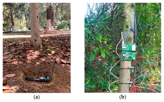
Figure 6.
Actual sensor node installation diagram: (a) deployment of the soil MC node; (b) testing of the wireless AE node.
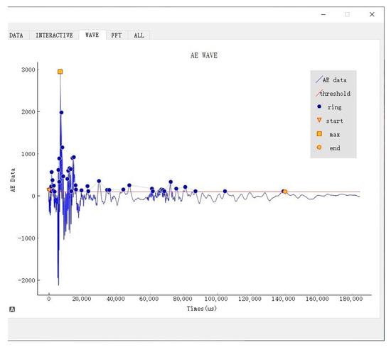
Figure 7.
Display interface of AE data.
First, refer to the international standard ISO 13061-1:2014 [35]; the beech samples with MC levels of 10%, 15%, 20%, 25%, 30%, 35%, 40%, 45%, and 50% (error ± 2%) were prepared correspondingly. The WASN nodes, as shown in Figure 3, were used to collect the AE parameters. Note that the wood samples and AE sensors were coupled by Vaseline to enhance the signal transmission capability. The AE nodes were sampled 100 times for each of the 9 specimens, and every set of data contained the following outputs of the near/far-end AE signals: amplitude, rise time, duration, ring count, and energy, along with the difference value between the near/far-ends signal, which was 15 parameters in all. Some of the results are presented below in Figure 8.
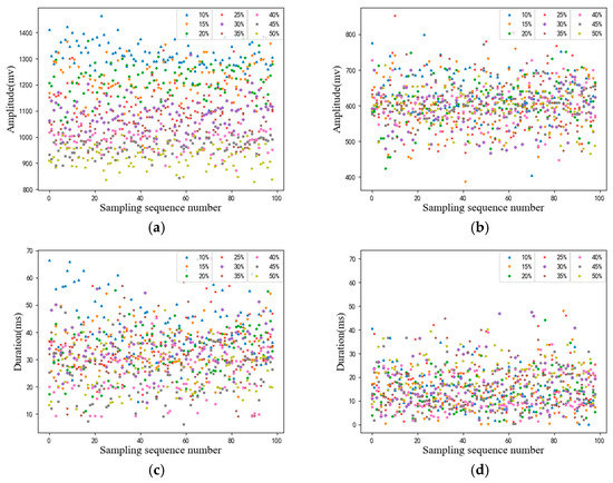
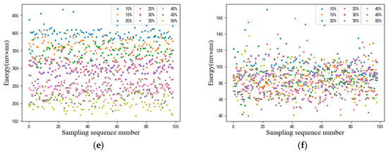
Figure 8.
AE results of wood samples with different MC levels: (a) amplitude of the near AE point; (b) amplitude of the far AE point; (c) duration of the near AE point; (d) duration of the far AE point; (e) energy of the near AE signal; (f) energy of the far AE signal.
Afterward, the original AE dataset should be normalized to values between [0, 1]:
where xmin, xmax, are the minimum and maximum values of input feature data, and xi* and xi are the normalized data and original data.
2.6.3. Feature Analysis
Based on the above data collection steps, the dataset matrix of soil and AE feature parameters (900 × 18) has been efficiently constructed, which should be used as the input of the mRMR selection module. Meanwhile, the corresponding MC level tags constituted the individual category vector accordingly. Here, if assuming that the number of optimal feature subset is 18, then the ranking order of all soil and AE features are lined up in Table 1 below.

Table 1.
Feature selection result of the mRMR.
Furthermore, when the number of optimal features gradually increased from the minimum to the maximum, an SVM training and testing configured with default parameters, and the corresponding recognition accuracy would be obtained, as shown in Figure 9. The analysis indicates that when the top nine features are used to construct the feature subsets, the recognition accuracy reaches an optimum value of 92.3%, and after that, the accuracy declines rapidly. Therefore, the first nine features obtained by the mRMR selection module are adopted to participate in the MC diagnosis procedure afterward.
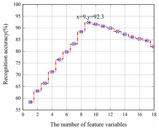
Figure 9.
Classification accuracy under feature sets with different scopes.
2.6.4. The FA-ISSA-SVM Diagnosis Algorithm
The sparrow search algorithm (SSA) proposed by reference [36] is an efficient swarm intelligence optimization mechanism. Compared with other methods, the SSA has the advantage of high searching accuracy, good stability, and strong robustness, but it also has the shortcoming of slow convergence speed. Based on this, the SSA algorithm was applied to the parameter optimization of the SVM, and a firefly perturbation strategy [37] was added to update the sparrow’s positions to further enhance the working efficiency. Taking the highest recognition accuracy of the SVM as the optimization object, the optimum regularization factor and kernel parameters were selected to establish the FA-ISSA-SVM diagnostic model.
The SSA mainly simulates the process of sparrow’s foraging, and it divides the population into three groups: discoverer, follower, and scouter. Discoverers have high fitness, a wide search range, and guide the sparrows to search and forage; followers forage with the discoverers to gain greater fitness; and the scouter will sound an alarm when it sees danger, and then the entire population makes an anti-predation behavior. Among the three groups, discoverers and followers could exchange roles with each other, whereas their proportion in the population remains constant, i.e., discoverers usually take up 10~20% of the entire colony.
Suppose there are N sparrows in a D-dimensional search space, the position of the K sparrow is Xk = [xk1, …, xkd, …, xkD], where xkd represents the position of the K-th sparrow in the d dimension. The discoverer should update its position as follow:
Here, t represents the current iteration number, itermax is the maximum number of iterations, represents the fitness of the k sparrow in the t + 1 generation, a is a random number ∈ (0, 1], R2 represents the warning value, ST represents the safety threshold, Q is a random number subject to the standard normal distribution, and L is a one-row, multidimensional, all-for-one matrix. When R2 < ST, no predators or other dangers are found for the sparrows, and the search environment is safe. The discoverer can search extensively to guide the population to obtain higher fitness. When R2 ≥ ST, the scouters find the predator and release the danger signal immediately, and the population performs an anti-predation act, adjusts the searching strategy, and moves to the safe area quickly. The position of followers is updated as follows:
In Equation (18), represents the worst position in the t-th iteration of the population, represents the optimal position in the t + 1 iteration of the population, A is 1 × d matrix with only 1 or −1 elements, and A+ = AT(AAT)−1. Scouter positions are updated as follows:
β is the step size control parameter, K is a random number belonging to [−1, 1], fk represents the fitness value of the K-th sparrow, and fg and fw are the best and worst current fitness, respectively.
Nevertheless, since the SSA may fall into the local optimum during the optimization process and thus reduce accuracy, the Firefly Algorithm (FA) is adopted to optimize the SSA for improving the optimization accuracy. The firefly perturbation strategy is applied to the sparrow population, and each individual searches for the most attractive individual in the population, that is, the individual with the best fitness value, based on the movement pattern of the relative brightness of the fireflies.
The relative fluorescence brightness of firefly I should be:
I0 is the maximum fluorescence brightness, which is proportional to the fitness value, and is the absorption coefficient of light intensity. rij is the relative distance between firefly individuals i and j.
Next, the firefly mutual attraction is:
In Equation (21), is the maximum attraction.
Then, the firefly disturbance position updating is shown:
In Equation (22), xi and xj are the spatial positions of sparrow i and j; σ is the step control parameter; and [0, 1] is a random factor subject to a uniform distribution.
Figure 10 shows the working process of the FA-ISSA-SVM, especially the optimization procedure for parameters C and γ. After the above procedures, the population size, maximum number of iterations, and SVM parameters of the FA and SSA can be initialized. Next, the fitness of individual sparrows is calculated to update the positions of discoverers, followers, and scouters. Then, we compare the advantages and disadvantages of the new position after firefly perturbation with the previous generation’s optimal value until the termination condition is met. Finally, the optimal SVM parameters are output to establish the FA-ISSA-SVM-based MC diagnosis model for practical measurement.
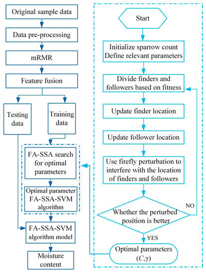
Figure 10.
Flowchart of the FA-ISSA-SVM algorithm.
3. Results and Discussion
The offline training shown in Figure 5 has been carried out in the gateway server, and the online identification should be implemented on different species of trees through the WASN sensor and soil MC nodes. The main process is as follows. Firstly, the sample dataset collected by sensors is preprocessed and normalized to be dimensionless. Next, the most representative nine characteristic parameters are screened from the sample dataset by the mRMR algorithm. Then, the feature fusion procedure is executed by weighing these selected features, and the optimal MC diagnosis model is trained by the FA-ISSA-SVM mechanism. Finally, real-time AE signals, root-soil moisture, air temperature, and air humidity data are input into the model to diagnose the MC level in the heart of the standing trees.
3.1. Algorithm Validation and Comparison
The WASN and soil moisture sensors were used to collect the corresponding parameters of phytophysiology and root-soil. A total of 900 groups were randomly divided into training groups and test groups at a ratio of 7:3, of which 630 were training groups and 270 were test groups. In order to verify the effectiveness of the feature selection algorithm and the superiority of the FA-ISSA-SVM MC diagnosis model, the following two categories of tests were executed. (1) In part one, the MC detection results of the features selected by the Pearson correlation coefficient method [38] and the features selected by the mRMR method were analyzed and compared, while the subsequent identification adopted the SVM with default configurations in common. (2) In part two, the detection results of the SVM, the genetic algorithm optimized SVM (GA-SVM) [39], the grid search algorithm optimized SVM (GS-SVM) [40], and the improved sparrow algorithm optimized SVM (FA-ISSA-SVM) [41] were analyzed. The feature vectors used for training are uniformly based on the selected results of the mRMR.
In both tests, recognition accuracy and the Kappa coefficient were used as the evaluation indexes. The accuracy rate refers to the proportion of correctly classified samples to the total test samples. The Kappa coefficient represents the proportion of classification error reduction in the classification result of the algorithm compared with the completely random classification result, and its value is between −1 and 1. The larger the value is, the better the ranking effect will be.
3.2. Feature Selection Performance Analysis
The Pearson correlation coefficient can reflect the degree of correlation between two characteristic variables and is defined as the quotient of covariance between variables and their standard deviation product. The closer the absolute value of the coefficient is to 1, the stronger the correlation between the two variables is. The closer the absolute value of the coefficient is to 0, the weaker the correlation is. Here, in order to verify the superiority of the mRMR selection method, the Pearson correlation coefficient has been employed for comparison.
X and Y in (23) are two individual characteristic parameters, is the standard deviation, and Cov(X, Y) is the corresponding covariance. The correlation between each two of the first eighteen characteristic parameters in this paper can be obtained by calculation according to (23), and its correlation analysis heat map is shown in Figure 11.
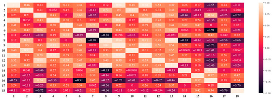
Figure 11.
Correlation analysis heat map.
Obviously, there existed considerable correlations in some parameters, including he near-end amplitude and the amplitude difference, the near-end energy and the energy difference, the far-end duration, and the far-end energy, et al. So, we also increased the optimal selected features from the minimum to maximum and recorded the subsequent identification accuracy, as shown in Table 2.

Table 2.
The SVM results of Pearson and mRMR feature selection.
The results in Table 2 show that the 11-dimensional features selected by Pearson’s correlation coefficient method obtained the best identification effect, although its accuracy rate is only 83.3% and the Kappa coefficient is 0.7435. By using the features of the mRMR choosing procedure, the accuracy was improved to 92.3%, and the Kappa coefficient was improved to 0.8624. Compared with Pearson’s method, the feature dimension of the mRMR algorithm is lower and the recognition accuracy is higher, which proves its efficiency and effectiveness in the feature selection part of the designed system.
3.3. Data Fusion Performance
The above section shows that the feature subset selected by the mRMR has achieved an efficient effect. Here, we further study the issue of whether the feature data fusion with entropy weight improves the dataset quality.
The proposed method with an entropy weight fusion mechanism and the other contrasting method without fusion are adopted for testing and comparing, respectively. They both use the original 630 group data as the input, while the mRMR step is carried out subsequently. Afterward, the two processes are executed and tested on each of the 270 groups. The corresponding results are displayed in Figure 12.
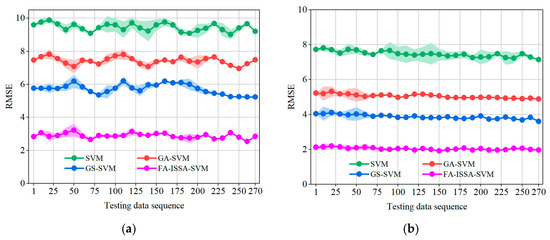
Figure 12.
Comparison of data fusion function: (a) detection results without data fusion; (b) detection results with data fusion.
In this part, the average validation indicator root-mean-square error (RMSE) and confidence interval are used for observation. We notice that in the two figures, the RMSE of the four SVMs after entropy weight data fusion decreased by about 25% compared with the unfused data. More obviously, the fluctuation of all RMSEs decrease, especially the confidence interval of the FA-ISSA-SVM, which approaches zero, which could be almost ignored. The reason is that the advantage of the entropy weight data fusion adopted in this paper lies in the dynamic allocation of the fusion weights according to the difference between the original information entropy and the conditional information entropy, which can achieve the optimal effect of minimum error fluctuation in the global data fusion.
3.4. Algorithm Comparison
The four algorithms all use the corresponding sample dataset after entropy weight feature fusion as the training input, and the experimental results are shown in Table 3. As can be seen, the recognition accuracy values of the optimized SVM algorithms are higher than the conventional SVM algorithm. The result of the traditional SVM is 89.16%, and after optimization by GS and GA, the accuracy rates are roughly improved to 93.32% and 93.25%. Finally, the FA-ISSA-SVM algorithm adopted performs the best, with an accuracy of 96.21%. The corresponding penalty factor C is 46.25, and the kernel parameter γ is 8.19.

Table 3.
Improvement strategies of the GWO.
In terms of working efficiency, the shortest iteration time of the SVM is 3.56 s. For the optimized SVM mechanisms, the shortest duration is 8.23 s for the FA-ISSA-SVM and is nearly half of the time of the GA-SVM and GS-SVM. So, the proposed method could effectively gain the highest recognition accuracy with a satisfying time cost.
3.5. Long-Term Field Evaluation
Afterward, to verify the reliability of the proposed multi-sensory information fusion system for the living trees, commercial equipment is adopted to calibrate the true values of MC level, the KT-80, a dual-function wood moisture measuring instrument from KLORTNER Technology, Italy [42]. We have carried out a measurement campaign on four typical tree species in Nanjing Forestry University (metasequoia, lodgepole pine, hovenia acerba, and a cherry–apple tree) in a monthly cycle from October 2021 to November 2022. The collected data includes the AE parameters, the root MC value, air humidity, and temperature. Because of the numerical fluctuation caused by seasonal variation, the FA-ISSA-SVM and the other six models (GA-SVM, GS-SVM, SVM, RF, KNN, Bayes) were used to analyze the feature parameters and compare identification performance. The final recognition accuracies were 96.4%, 96.7%, 96.3%, and 95.5%, respectively. Figure 13 shows the diagnostic process of the metasequoia with an accuracy of 96.4% as a demonstration, where the solid line represents the average MC of seven algorithms for metasequoia at the very month, the shaded part is the error band area, and the dotted line represents the average of the MC for the quarter. So, we can see and compare both MC variations during the months and quarters.


Figure 13.
Prediction results of the MC in different seasons by seven algorithms with selected characteristic parameters.
According to the practical testing data and predicted value, the average MC reached a maximum of 42.3% in summer, while the average MC in spring and autumn decreased to 39.7% and 38.2%, respectively. Of course, the lowest value was 36.2% in winter. Due to the influence of long-term light conditions, high temperature, CO2, and other environmental factors in summertime, the effective photosynthesis and transpiration rate of living trees have increased to a certain extent; thus, the MC level of living tree trunks also increases.
Compared with other recognition models, the final results of the FA-ISSA-SVM in one year are closer to the calibrating data. In addition, the FA-ISSA-SVM has an excellent performance in terms of error band interval, and its error band area is far smaller compared to other algorithms, which also means that the data obtained by the FA-ISSA-SVM fluctuates within a credible range.
Next, to further verify the prediction performance of these models, multiple indicators of the RMSE, mean absolute error (MAE), mean absolute percentage error (MAPE), and goodness-of-fit (R2) were employed for the evaluation. Compared with Bayes, RF, KNN, SVM, GS-SVM, GA-SVM, and the FA-ISSA-SVM model show optimal diagnostic accuracy with high stability; specific data are shown in Figure 14.

Figure 14.
Evaluation index chart of seven diagnostic models.
3.6. Short-Term Field Evaluation
The annual MC of living wood trunks is worthy of attention, as MC statuses change throughout the day. August is a relatively important stage for the growth and development of trees, and the physiology of trees is very active. Therefore, we selected two consecutive days (21 August 2022 to 22 August 2022) when the meteorological environment (including rainfall, wind speed, wind direction, air pressure, etc.) has little change and conducted continuous monitoring for 48 h. The diagnostic system was set up on four different tree species. We envisagd that the FA-ISSA-SVM can maintain the best generalization ability and robustness even in the most active stage of the physiological activity of trees, which means that the FA-ISSA-SVM has good applicability under different working conditions. The MC predicted by different models and the calibrated real MC value of the four tree species are shown in Figure 15.
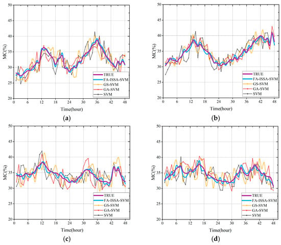
Figure 15.
Trunk MC variations of four trees during 48 h: (a) MC records of metasequoia; (b) MC records of lodgepole pine; (c) MC records of hovenia acerba; (d) MC records of cherry–apple.
Results show that the highest MC of the four trees mostly occurs around noon, when the temperature is the highest, the sun’s effective radiation is the strongest, and the tree’s transpiration rate is the highest. The MC of the cherry–apple tree appears at two peaks in one day, which may be affected by the intercellular CO2 and stomatal restrictions. When the trunk’s water content has saturated to a certain extent, the phenomenon of “midday depression of photosynthetic” appears.
3.7. The Superiority of the Multi-sensory Data Fusion System
The proposed multi-sensory data fusion system for non-destructive MC detection compares favorably with previous methods for the monitoring of field standing trees.
Firstly, all the characteristic parameters required for the detection are collected in a non-destructive way, without causing irreversible damage to the standing trees.
Secondly, the structural differences between the surface and interior of the standing trees result in significant noise when the AE signal propagates inside the trunk with its inhomogeneous, porous, and anisotropic nature. Here, we used Vaseline to couple the acquisition sensor and live tree trunk during installation. On the one hand, the acquisition system is highly sensitive, the distance between the AE probes and the sound source is very close (10 cm/20 cm), and the three sensing devices are mounted in one straight line, which reduces the interference noise at the physical level and fully retains the effective AE signal. On the other hand, when the AE signal propagates along the tree bark, the interference for the original signal is further averted and reaches the optimal propagation path. At this point, the impact of AE signal noise can be weakened as much as possible. This is also the reason why AE signals on the bark of the trunk were collected.
Thirdly, the power consumption of the proposed WASN in this paper mainly includes three parts: AE signal source (i.e., the vibrating motor), AE signal acquisition, and LoRa wireless communication. The rated operating voltage and current of the micro-vibration motor are 3.3 V and 85 mA, respectively, which means its power consumption is about 280.5 mW. The LoRa module SX1278 has a maximum transmitting power of 100 mW. The power consumption of the analog-to-digital converter AD7356 and the preamplifier OPA627 chip is about 111 mW. Hence, the energy consumption of the whole WASN system in a working state is about 492 mW. Moreover, the WSAN nodes have two modes: working and sleeping. Their duty cycle is usually set at about 3%, and considering that the node only needs to collect data every 6 h, it can be calculated that the power consumption is about 2000 mW per day. When using a 3.7 V 30 Ah lithium battery pack, one WASN node can operate normally for 55.5 days. Therefore, the designed WASN basically meets the application requirements for forestry field monitoring.
Meanwhile, the soil sensor node adopts a 5 V rechargeable lithium battery, and it also has two modes of work and sleep. After data collection, the node will enter sleeping mode immediately. The soil node can work normally for 15 h under full voltage through lab testing, and the working time is about 8 min per day; thus, the soil node can last for 112 days after installation, which fully shows its reliability and stability in the forest IoT scenario.
4. Conclusions
In this paper, a non-destructive diagnosis strategy for the standing tree MC level based on a multi-sensory information fusion system was studied. The mRMR was used to select optimal features from the root-soil and AE signal parameters. Feature fusion was carried out based on the weight of conditional information entropy, and the FA-ISSA-SVM deduction model was constructed. The system optimized the SVM operation parameters based on the fusion feature subset and achieved an accurate identification rate. By comparison and evaluation of the long-term measurement, the following conclusions can be drawn:
- (1)
- The mRMR algorithm was highly efficient for the hybrid features’ optimal selection procedure. When the first nine features were input into the recognition model, the accuracy of the SVM for the collected data was more than 92%.
- (2)
- After the conditional entropy weight information fusion, the diagnostic model dynamically adjusts the data fusion weighting coefficient of the corresponding sensor characteristic parameters according to the variance changes of the measured values of each sensor, and finally obtains a minimum root-mean-square error of 2.23% and a maximum goodness-of-fit of 97.64%.
- (3)
- The proposed system performed an excellent steady-state precision and generalization performance for the online MC diagnosis of living trees’ heartwood. When applied on the metasequoia, lodgepole pine, hovenia acerba, and cherry–apple trees, respectively, the diagnosis accuracy reached 96.4%, 96.7%, 96.3%, and 95.5%.
- (4)
- By comparison with the commercial MC measuring instrument, the proposed system can effectively represent the average MC level of the trunk and has stronger applicability to the living trees in the field with a high MC value.
Author Contributions
Z.Y. and Y.W. devised the programs together; Z.Y. drafted the initial manuscript and designed the project; Y.W. and Y.L. revised the manuscript. All authors have read and agreed to the published version of the manuscript.
Funding
This work was supported in part by the National Natural Science Foundation of China by grant 32171788 and 31700478, and China’s Jiangsu Provincial Government Scholarship for Overseas Study by grant JS-2018-043.
Institutional Review Board Statement
Not applicable.
Informed Consent Statement
Not applicable.
Data Availability Statement
Not applicable.
Conflicts of Interest
The authors declare no conflict of interest.
References
- Rivers, M.; Newton, A.C.; Oldfield, S. Scientists’ warning to humanity on tree extinctions. Plants People Planet 2022, 2572–2611. [Google Scholar] [CrossRef]
- Cienciala, E.; Russ, R.; Santruckova, H.; Altman, J.; Kopacek, J.; Hunova, I.; Stepanek, P.; Oulehle, F.; Tumajer, J.; Stahl, G. Discerning environmental factors affecting current tree growth in Central Europe. Sci. Total Environ. 2016, 573, 541–554. [Google Scholar] [CrossRef] [PubMed]
- Alavi, G. The impact of soil moisture on stem growth of spruce forest during a 22-year period. For. Ecol. Manag. 2002, 166, 17–33. [Google Scholar] [CrossRef]
- Tian, Y.; Zhang, Q.L.; Liu, X.; Meng, M.; Wang, B. The Relationship between Stem Diameter Shrinkage and Tree Bole Moisture Loss Due to Transpiration. Forests 2019, 10, 290. [Google Scholar] [CrossRef]
- Edwards, W.; Jarvis, P. A method for measuring radial differences in water content of intact tree stems by attenuation of gamma radiation. Plant Cell Environ. 1983, 6, 255–260. [Google Scholar]
- Namken, L.N.; Lemon, E. Field Studies of Internal Moisture Relations of the Corn Plant 1. Agron. J. 1960, 52, 643–646. [Google Scholar] [CrossRef]
- Byrne, G.; Fenn, M.; Burgar, M. Nuclear magnetic resonance studies of water in tree sections. Agric. For. Meteorol. 1986, 38, 307–317. [Google Scholar] [CrossRef]
- Constantz, J.; Murphy, F. Monitoring moisture storage in trees using time domain reflectometry. J. Hydrol. 1990, 119, 31–42. [Google Scholar] [CrossRef]
- Holbrook, N.M.; Burns, M.; Sinclair, T. Frequency and time-domain dielectric measurements of stem water content in the arborescent palm, Sabal palmetto. J. Exp. Bot. 1992, 43, 111–119. [Google Scholar] [CrossRef]
- He, H.; Turner, N.C.; Aogu, K.; Dyck, M.; Feng, H.; Si, B.; Wang, J.; Lv, J. Time and frequency domain reflectometry for the measurement of tree stem water content: A review, evaluation, and future perspectives. Agric. For. Meteorol. 2021, 306, 108442. [Google Scholar] [CrossRef]
- Yunjie, X. Wireless sensor monitoring system of Canadian Poplar Forests based on Internet of Things. Artif. Life Robot. 2019, 24, 471–479. [Google Scholar] [CrossRef]
- Vikash; Varma, S. Trust-based forest monitoring system using Internet of Things. Int. J. Commun. Syst. 2019, 35, e4163. [Google Scholar]
- Lazarescu, M.T. Design of a WSN Platform for Long-Term Environmental Monitoring for IoT Applications. IEEE J. Emerg. Sel. Top. Circuits Syst. 2013, 3, 45–54. [Google Scholar] [CrossRef]
- Algobail, A.; Soudani, A.; Alahmadi, S. Energy-aware Scheme for Animal Recognition in Wireless Acoustic Sensor Networks. In Proceedings of the 7th International Conference on Sensor Networks, Funchal, Portugal, 22–24 January 2018; pp. 31–38. [Google Scholar]
- Xu, W.; Zhang, X.; Yao, L.; Xue, W.; Wei, B. A Multi-view CNN-based Acoustic Classification System for Automatic Animal Species Identification. Ad Hoc Netw. 2020, 102, 102115. [Google Scholar] [CrossRef]
- Wu, Y.; Tian, G.; Liu, W. Research on Moisture Content Detection of Wood Components Through Wi-Fi Channel State Information and Deep Extreme Learning Machine. IEEE Sens. J. 2020, 20, 9977–9988. [Google Scholar] [CrossRef]
- Tao, K.; Zheng, W. Automatic selection of low-permeability sandstone acoustic emission feature parameters and its application in moisture identification. Appl. Sci. 2018, 8, 792. [Google Scholar] [CrossRef]
- Wei, Z.; Jiang, J.; Kai, T. A Method based on Musical-staff-inspired Signal Processing Model for Measuring Rock Moisture Content. Measurement 2018, 125, 577–585. [Google Scholar]
- Li, H.; Shen, R.; Li, D.; Jia, H.; Hou, Z. Acoustic Emission Multi-Parameter Analysis of Dry and Saturated Sandstone with Cracks under Uniaxial Compression. Energies 2019, 12, 1959. [Google Scholar] [CrossRef]
- Naderi-Boldaji, M.; Tekeste, M.Z.; Nordstorm, R.A.; Barnard, D.J.; Birrell, S.J. A mechanical-dielectric-high frequency acoustic sensor fusion for soil physical characterization. Comput. Electron. Agric. 2019, 156, 10–23. [Google Scholar] [CrossRef]
- Tate, B.L. Soil Texture Determination by an Acoustic Cone Penetrometer Method. Master’s Thesis, University of Illinois, Urbana, IL, USA, 2016. [Google Scholar]
- Sharma, G.; Kumar, M.; Verma, S. Monitoring deforestation using acoustic signals. In Proceedings of the 2016 International Conference on Bioinformatics and Systems Biology (BSB), Allahabad, India, 4–6 March 2016. [Google Scholar]
- De Roo, L.; Vergeynst, L.L.; De Baerdemaeker, N.J.F.; Steppe, K. Acoustic Emissions to Measure Drought-Induced Cavitation in Plants. Appl Sci. 2016, 6, 71. [Google Scholar] [CrossRef]
- Peeters, B. The Use of Acoustic Emissions in Drought-Induced Cavitation Research: Establishing a Link between AE and Visually Detected Embolisms via X-ray Computed Microtomography in Prunus avium L. Master’s Thesis, Gent University, Gent, Belgium, 2017. [Google Scholar]
- Kageyama, K.; Kojima, K.; Nakamura, T. AE Measurement Approach for Activity Monitoring of Foliage Plants. In Proceedings of the 2017 IEEE 6th Global Conference on Consumer Electronics (GCCE), Nagoya, Japan, 24–27 October 2017. [Google Scholar]
- Ozbey, B.; Eibert, T.F. Wireless Non-Destructive Moisture Content Characterization of Trees by Highly-Sensitive Compact Resonating Probes. IEEE Sens. J. 2020, 21, 6125–6132. [Google Scholar] [CrossRef]
- OPA627, Texas Instruments Co., Ltd., USA. Available online: https://www.ti.com.cn/product/cn/OPA627 (accessed on 20 April 2023).
- AD7356, Analog Devices Co., Ltd., USA. Available online: https://www.analog.com/cn/products/ad7356.html (accessed on 20 April 2023).
- STM32F405RG, STMicroelectronics Co., Ltd., Switzerland. Available online: https://www.st.com/en/microcontrollers-microprocessors/stm32f405rg.html (accessed on 20 April 2023).
- SX1278, Sentech Co., Ltd., USA. Available online: https://www.semtech.cn/products/wireless-rf/lora-connect/sx1278 (accessed on 20 April 2023).
- Liu, Y.; Wu, Y.; Liu, W.; Liu, Y. Diagnostic method of water content of living wood based on wireless acoustic emission sensor system. J. Electron. Meas. Instrum. 2022, 36, 160–168. [Google Scholar]
- Liu, K.; Zhang, T.; Zhang, R.; Yu, S.; Huang, L.; Jiang, S.; Hu, D. Characteristics of tree-ring density change and its response to climate at different tree heights. Chin. J. Appl. Ecol. 2021, 32, 503–512. [Google Scholar]
- Luo, C.; Zha, T.; Zhu, M.; Zhu, Z.; Wang, Z.; Liu, W. Effects of shallow groundwater on trunk sap flow of riparian poplar forests in North China. Chin. J. Appl. Ecol. 2016, 27, 1401–1407. [Google Scholar]
- Chui, J.; You, X.; Zhang, D.; Zhang, L.; Zhang, J.; Fu, R. Spatial distribution characteristics of coarse roots of main street trees in Shanghai and their relationship with site environment. J. Yunnan Agric. Univ. 2023, 38, 272–282. [Google Scholar]
- 13061-1:2014; Physical and Mechanical Properties of Wood—Test Methods for Small Clear Wood Specimens. International Organization for Standardization: Geneva, Switzerland, 2014.
- Xue, J.; Shen, B. A novel swarm intelligence optimization approach: Sparrow search algorithm. Syst. Sci. Control. Eng. Open Access J. 2020, 8, 22–34. [Google Scholar] [CrossRef]
- Ren, X.Y.; Chen, S.; Wang, K.Y.; Tan, J. Design and application of improved sparrow search algorithm based on sine cosine and firefly perturbation. Math. Biosci. Eng. 2022, 19, 11422–11452. [Google Scholar] [CrossRef]
- Zhang, S.R.; Bai, X.Y.; Zhao, C.W.; Tan, Q.; Luo, G.J.; Cao, Y.; Deng, Y.H.; Li, Q.; Li, C.J.; Wu, L.H.; et al. Limitations of soil moisture and formation rate on vegetation growth in karst areas. Sci. Total Environ. 2022, 810, 10. [Google Scholar] [CrossRef]
- VanDeventer, W.; Jamei, E.; Thirunavukkarasu, G.S.; Seyedmahmoudian, M.; Soon, T.K.; Horan, B.; Mekhilef, S.; Stojcevski, A. Short-term PV power forecasting using hybrid GASVM technique. Renew. Energy 2019, 140, 367–379. [Google Scholar] [CrossRef]
- Hou, S.K.; Liu, Y.R.; Yang, Q. Real-time prediction of rock mass classification based on TBM operation big data and stacking technique of ensemble learning. J. Rock Mech. Geotech. Eng. 2022, 14, 123–143. [Google Scholar] [CrossRef]
- Yan, H.; Zhang, J.X.; Zhou, N.; Shi, P.T.; Dong, X.J. Coal permeability alteration prediction during CO2 geological sequestration in coal seams: A novel hybrid artificial intelligence approach. Geomech. Geophys. Geo-Energy Geo-Resour. 2022, 8, 11. [Google Scholar] [CrossRef]
- KT-80, KLORTNER Technology Co., Ltd., Italy. Available online: https://www.ize-industries.com/product7-746-82-924-0.html (accessed on 20 April 2023).
Disclaimer/Publisher’s Note: The statements, opinions and data contained in all publications are solely those of the individual author(s) and contributor(s) and not of MDPI and/or the editor(s). MDPI and/or the editor(s) disclaim responsibility for any injury to people or property resulting from any ideas, methods, instructions or products referred to in the content. |
© 2023 by the authors. Licensee MDPI, Basel, Switzerland. This article is an open access article distributed under the terms and conditions of the Creative Commons Attribution (CC BY) license (https://creativecommons.org/licenses/by/4.0/).