Anomaly Detection of Remote Sensing Images Based on the Channel Attention Mechanism and LRX

Abstract

Anomaly detection of remote sensing images has gained significant attention in remote sensing image processing due to their rich spectral information. The Local RX (LRX) algorithm, derived from the Reed–Xiaoli (RX) algorithm, is a hyperspectral anomaly detection method that focuses on identifying anomalous pixels in hyperspectral images by exploiting local statistics and background modeling. However, it is still susceptible to the noises in the Hyperspectral Images (HSIs), which limits its detection performance. To address this problem, a hyperspectral anomaly detection algorithm based on channel attention mechanism and LRX is proposed in this paper. The HSI is feed into the auto-encoder network that is constrained by the channel attention module to generate a more representative reconstructed image that better captures the characteristics of different land covers and has less noises. The channel attention module in the auto-encoder network aims to explore the effective spectral bands corresponding to different land covers. Subsequently, the LRX algorithm is utilized for anomaly detection on the reconstructed image obtained from the auto-encoder network with the channel attention mechanism, which avoids the influence of noises on the anomaly detection results and improves the anomaly detection performance. The experiments are conducted on three HSIs to verify the performance of the proposed method. The proposed hyperspectral anomaly detection method achieves higher Area Under Curve (AUC) values of 0.9871, 0.9916 and 0.9642 on HYDICE urban dataset, AVIRIS aircraft dataset and Salinas Valley dataset, respectively, compared with other six methods. The experimental results demonstrate that the proposed algorithm has better anomaly detection performance than LRX and other algorithms.

1. Introduction

Hyperspectral images (HSIs) are composed of hundreds of continuous narrow spectral bands that cover the visible band to Near Infrared (NIR) or Short Wave Infrared (SWIR) range [1]. These images exhibit unique spectral characteristics due to their continuous spectrum curves. Each land cover within the HSI has its own distinct continuous spectral curve, enabling the identification of subtle differences between different land covers. Therefore, HSIs find extensive applications in various fields, such as target detection, change detection and anomaly detection. The purpose of hyperspectral anomaly detection is to identify objects whose spectrum are significantly different from the surrounding background. The spectral features of anomalies in the HSI differ significantly from those of the surrounding pixels, and the entire image excluding the anomalies is considered as the background [2]. Hyperspectral anomaly detection typically falls under the category of unsupervised binary classification since it does not require prior knowledge or a priori information about the target or the background. Since the spectral information of many land covers cannot be known in advance, hyperspectral anomaly detection is highly relevant to real-world scenarios and has been successfully applied in various fields, such as civil search and rescue, precision agriculture, and mineral exploration [3,4,5].

Over the past decades, many hyperspectral anomaly detection algorithms have been proposed, which can be roughly classified into four categories: statistical-based algorithms, representation-based algorithms, matrix decomposition-based algorithms, and deep learning-based algorithms [6].

The RX algorithm, short for Reed–Xiaoli (RX) algorithm, is a classic statistical-based algorithm that assumes a Gaussian distribution for the background. It detects anomalies by calculating the spectral difference between the target pixel and the background pixel using the Mahalanobis distance. However, the RX algorithm calculates the covariance matrix for the entire image, which means it is influenced by the anomalous pixels in the overall background when calculating the Mahalanobis distance for a single pixel point. To address this issue, the Local RX (LRX) algorithm [7] employs a two-window sliding strategy. It extracts the background for each sliding window and calculates the covariance matrix specifically for that window. The Mahalanobis distance is then calculated within the sliding window to detect anomalies. Thus, the LRX algorithm can alleviate the problem that the RX algorithm is susceptible to other background. Dora and Majumdar [8] conducted a comparison of the RX algorithm based on different distances, namely the Bhattacharya distance, KL divergence, and Jeffrey divergence, to assess their impact on different spectral bands. Hidalgo et al. [9] proposed a nonlinear anomaly detection algorithm based on the RX algorithm and reproducing kernel theory. It should be noted that the RX algorithm assumes that the background obeys a multivariate Gaussian distribution [10,11], but HSIs in real scenes do not satisfy this assumption.

The representation-based algorithms assume that the background pixel in a HSI can be approximated using its surrounding pixels or a background dictionary, while anomalous pixels cannot be effectively represented. As a result, representation-based algorithms do not rely on assumptions about the distribution of HSIs, making them more suitable for real-world scenarios. Representation-based algorithms mainly contain algorithms based on a collaborative-based detector [12,13] and algorithms based on sparse representation [14].

The hyperspectral anomaly algorithm based on Low-rank and Sparse Matrix Decomposition (LRaSMD) [15] is a representative matrix decomposition-based algorithm. It assumes that the background in HSIs has a low-rank property and the anomalous target has a sparse property [16]. The LRaSMD algorithm employs matrix decomposition to obtain a sparse matrix and determines anomalous targets by calculating the Euclidean distance within the sparse matrix. Ruhan et al. [17] proposed an enhanced tensor RPCA-based Mahalanobis distance algorithm, which utilizes weighted tensor Schatten p-norm minimization and solves non-convex problems using Fourier transform, generalized soft-threshold, and a tensor singular value decomposition to address decomposition issues.

In recent years, deep learning techniques have gained significant attention for their promising detection performance in hyperspectral anomaly detection. Deep learning-based algorithms can be broadly classified into three major categories: convolutional neural network-based, generative adversarial network-based, and auto-encoder-based algorithms. Convolutional neural network-based algorithms train neural networks to distinguish the differences between adjacent pixels and utilize the trained network to detect anomalies based on pixel differences [18]. Generative adversarial network-based algorithms remove the background from HSIs by subtracting synthetic images from the original image, then detect anomalies based on the acquired spectral difference images [19]. The auto-encoder-based algorithms consists of an encoder and a decoder. Since the majority of the input data to the auto-encoder network are background pixels, the network learns patterns represent the background. The decoding and reconstruction of background pixels yield a low reconstruction error, while anomalous targets exhibit a considerably higher reconstruction error. This distinction serves as an effective method for detecting anomalies [20]. Zhao and Sun [21] proposed a memory-augmented auto-encoder for hyperspectral anomaly detection, where the latent representation from the auto-encoder is used to retrieve the most relevant matrix items in a memory matrix.

Although the auto-encoder network can better extract features from HSIs [22], it does not pay attention to the effective bands of land covers during the feature extraction process. Each land cover within HSIs exhibits different effective bands, and incorporating an attention mechanism can enhance the effectiveness of the extracted features by emphasizing the important bands for each land cover. Moreover, the performance of the LRX algorithm is easily affected by noise, while HSIs have high noise because of the low signal-to-noise ratio in hyperspectral sensors, environmental influences, and technical limitations during image acquisition. Due to the influence of noise, the direct application of the LRX method for anomaly detection on HSIs does not yield satisfactory results. Therefore, this paper proposes a hyperspectral anomaly detection algorithm based on the channel attention mechanism and LRX. The HSI is fed into the auto-encoder network that is constrained by the channel attention module to generate a more representative reconstructed image that better captures the characteristics of the land covers. The channel attention module in the auto-encoder network aims to explore the effective spectral bands corresponding to different land covers. Subsequently, the LRX algorithm is utilized for anomaly detection on the reconstructed image obtained from the auto-encoder network with the channel attention mechanism.

The main contributions of this paper include:

(1)

The channel attention module is proposed to explore the effective bands of HSIs, enhancing the representation of different land covers in the reconstructed image generated by the auto-encoder network.

(2)

The LRX algorithm is employed for anomaly detection on the reconstructed image, which effectively alleviates the impact of existing noises in HSIs.

(3)

The effectiveness of the proposed hyperspectral anomaly detection algorithm based on the channel attention model and LRX is verified on three hyperspectral datasets, HYDICE, AVIRIS, and Salinas, with AUC values of 0.9871, 0.9916, and 0.9642, respectively.

2. Related Work

2.1. Auto-Encoder Network

Auto-encoder is an unsupervised neural network model, which consists of two modules: the encoder and decoder. It is widely used for many tasks such as image reconstruction, clustering, and machine translation, dimensionality reduction, document retrieval, classification, and anomaly detection [23,24,25]. The auto-encoder aims to learn an efficient representation of the input data by compressing them into a lower-dimensional space and then reconstructing them back to their original form. During the encoding phase, the input data are processed by the encoder, which encodes and compresses them into hidden layer features. These hidden layer features represent the extracted features in the mapping process. Subsequently, the decoder decodes the hidden layer features to reconstruct the original data. By performing non-linear dimensionality reduction, the auto-encoder learns a mapping function to extract implicit features from the input data, effectively reducing noise in the original data. Bati et al. [26] proposed a hyperspectral anomaly detection algorithm based on the auto-encoder, which first represents hyperspectral backgrounds of different complexity with the auto-encoder. Then, the anomalies are detected by calculating the reconstruction error between the original image and the decoded image.

2.2. Channel Attention Mechanism

The attention mechanism, inspired by the human eye’s mechanism of observing external objects, only concentrates on some crucial local information of an image. In other words, it creates a mask to identify the important parts of an image, aiming to understand the weight distribution of features. The attention mechanism has already been applied in various fields such as natural language processing, machine translation, and classification.

Attention mechanisms can be roughly divided into three categories: spatial attention mechanism, channel attention mechanism, and spatial–channel attention mechanism. The spatial attention mechanism adjusts and calculates the weights by locating the target region in the image and performing affine transformations. The channel attention mechanism, on the other hand, adjusts weights based on the influence of different bands of the feature map on the output data [27]. The spatial–channel attention mechanism is a combination of the two above-mentioned mechanisms.

Hyperspectral images are characterized by low spatial resolution and high spectral resolution, and the uniqueness of their spectral characteristics provides the possibility to detect and identify targets. In order to better focus on the spectral features, this paper adopts the channel attention mechanism, which takes the spectral bands as input. Since the feature map of each channel contains different information, the response values of different land covers in different bands are different. Therefore, the channel attention mechanism can identify the different channel information of land covers and focus on more effective bands.

2.3. LRX Algorithm

The classical RX is a global hyperspectral anomaly detection algorithm. It calculates the Mahalanobis distance between the pixel to be detected and the mean value of the background to determine whether the pixel is anomalous. However, it is important to note that the covariance matrix in the RX algorithm is calculated based on all pixels in the image, treating the entire image as the background. As a result, it is susceptible to the influence of background pixels when calculating the Mahalanobis distance. On the other hand, the LRX algorithm is a local hyperspectral anomaly detection algorithm [28]. The detection window of LRX consists of a target window and a background window, with the background window being much larger than the target window. In the LRX algorithm, the covariance matrix is calculated in the region by subtracting the background window from the target window, which alleviates the problem that the RX algorithm is easily affected by background pixels.

Assuming that the number of bands of hyperspectral images is D, the background containing N pixel points can be represented as a matrix $X_b=[x_1,x_2,\cdots ,x_N]$ of size $N\times D$. Here, $x_i=[x_{1i},x_{2i},\cdots ,x_{Di}]$, where $x_{ni}$ denotes the spectrum of each pixel.

Suppose that $H0$ represents the scenario where the target does not exist, and $H1$ denotes the scenario where the target does exist.

$$\left\{\begin{array}{c}H0:x=n,\mathrm{when}\mathrm{the}\mathrm{target}\mathrm{does}\mathrm{not}\mathrm{exist}\hfill \\ H1:x=as+n,\mathrm{when}\mathrm{the}\mathrm{target}\mathrm{exists}\hfill \end{array}\right.,$$

(1)

where, x represents the vector of the pixel to be detected, n denotes the background noise vector, and s is the target spectrum vector.

$${\mu }_b=\frac{1}{N}{\sum }_{i=1}^N{x}_i,$$

(2)

$$C_b=\frac{1}{N}{\sum }_{i=1}^N(x-{\mu }_b){(x-{\mu }_b)}^T,$$

(3)

$$LRX\left(x\right)=(x-{\mu }_b)C_b^{-1}{(x-{\mu }_b)}^T,$$

(4)

where, ${\mu }_b$ represents the mean value of the background window, and $C_b$ represents the covariance matrix of the background window. The LRX detector calculates the Mahalanobis distance between the spectrum of the pixel to be detected and the mean vector of the background window. If the Mahalanobis distance exceeds a predefined threshold, the pixel is considered anomalous.

3. Hyperspectral Anomaly Detection Based on the Channel Attention Mechanism and LRX

In this paper, a hyperspectral anomaly detection algorithm based on the channel attention mechanism and LRX is proposed, as illustrated in Figure 1. The algorithm follows a two-step process: first, it obtains the reconstructed image using the auto-encode network with the channel attention mechanism, and then uses the LRX algorithm for anomaly detection on the reconstructed image. The auto-encode network based on the channel attention mechanism consists of two sub-networks: the channel attention network and the auto-encoder network. The channel attention network is designed to extract the effective bands of HSIs as input in order to focus on the separability of the spectral bands. Meanwhile, the auto-encode network performs encoding and decoding operations on the HSIs, incorporating the channel attention mechanism. This process can effectively reduce the noise and can generate the representative reconstructed image that accurately captures the characteristics of the land covers. Finally, the LRX algorithm is utilized to the representative reconstructed image to better detect anomalies.

3.1. Channel Attention Network

The channel attention network is shown in the left part of Figure 1. The channel attention matrix, denoted as $M_c$, can be obtained from the channel attention network. The process of the channel attention network is shown as follows.

First, the input image with dimensions $(H,W,D)$ is fed into the channel attention network, where H and W denote the spatial dimensions, and D represents the number of channels. Second, the global average pooling (AvgPool) and global maximum pooling (MaxPool) operations are applied to the input image along the spatial dimensions with the size of $H\times W$. These pooling operations aggregate information across the entire spatial extent, resulting in two matrices, both with a size of $1\times 1\times D$, namely $M_a$ and $M_m$. AvgPool calculates the average value for each channel, providing a measure of the average activation within each channel, while MaxPool identifies the maximum value for each channel, indicating the most salient activation within each channel. Third, The matrices $M_a$ and $M_m$ obtained from global pooling operations are fed into a fully connected network to extract important features $F_a$ and $F_m$, respectively. Fourth, the extracted feature vectors, $F_a$ and $F_m$, are combined by element-wise summation, resulting in a single combined feature vector. Finally, the combined feature vector is then passed through a sigmoid activation function, which allowing the model to assign weights or importance coefficients to different channels. The output of the sigmoid activation function represents the weight coefficients associated with each channel. These coefficients are used to generate the channel attention matrix, denoted as $M_c$, with dimensions $1\times 1\times D$. Therefore, the channel attention matrix captures the relative importance of each channel in the input data. By incorporating the channel attention matrix into the proposed network, the model can effectively emphasize relevant channels and suppress irrelevant ones during the feature extraction process, which helps to enhance the discriminative power of the network and improve hyperspectral anomaly detection performance. The channel attention matrix $M_c$ can be calculated by Equation (5).

$$M_c=Sigmoid(Dense\left(AvgPool\left(F\right)\right)+Dense\left(Maxpool\left(F\right)\right)),$$

(5)

3.2. Auto-Encoder Network

The auto-coder network is illustrated in the right part of Figure 1 and comprises two components: the encoder and the decoder. The encoder consists of three Dense layers with a neuron configuration of [128, 64, 32], along with an intermediate hidden layer containing 16 neurons. Similarly, the decoder consists of three Dense layers with [32, 64, 128] neurons. The specific network structure is shown in

Table 1. Network structure.

Name	Output Size	Activation Function
Input$X$	$N\times D$
Dense	$N\times 128$	RELU
Dense	$N\times 64$	RELU
Dense	$N\times 32$	RELU
Dense Z	$N\times 16$	RELU
Dense	$N\times 32$	RELU
Dense	$N\times 64$	RELU
Dense	$N\times 128$	RELU
Output$X^{{}^{\prime }}$	$N\times D$

, where $N=H\times W$.

First, the channel attention matrix $M_c$ is element-wise multiplied with the input image F, resulting in $Input=M_c\odot F$. Reshaping this resulting matrix to dimensions $N\times D$ yields the input matrix X, where $N=H\times W$. Second, the input matrix X is sequentially passed through each Dense layer and the intermediate hidden layer of the encoder. The outputs are of size $(N,128)$, $(N,64)$, $(N,32)$, and $(N,16)$, respectively. Third, the output Z of the intermediate hidden layer with a size of $(N,16)$ can be calculated by Equation (6), where w and b represent the weights and biases of the encoder layers. Fourth, Z is fed through each Dense layer of the decoder. The corresponding outputs are of size $(N,32)$, $(N,64)$, and $(N,128)$, respectively. Finally, the number of neurons in the last Dense layer matches the number of bands D, resulting in the reconstructed feature matrix $X^{{}^{\prime }}$ with the size of $N\times D$. $X^{\prime }$ can be calculated by Equation (7), where $\tilde{w}$ and $\tilde{b}$ represent the weights and biases of the decoder layers. Reshaping $X^{\prime }$ to dimensions $H\times W\times D$ yield the reconstructed image $\widehat{F}$. The auto-encoder performs non-linear dimensionality reduction by learning a mapping function that extracts implicit features from the input image. This process effectively reduces noises in the input image and generates the reconstructed image with less noise.

$$Z=f(X,w,b),$$

(6)

$$X^{{}^{\prime }}=f(Z,\tilde{w},\tilde{b}),$$

(7)

The loss function employed is the root mean square error to jointly train the channel attention network and the auto-encoder network. The initial learning rate is set to 0.0004, and the Adam optimizer is utilized for training. The number of training epochs is set between 10 and 300 depending on the specific datasets. The proposed channel attention network and the auto-encoder are implemented using the PyTorch framework. To conduct the comparison experiments, a PC equipped with an Intel(R) Core(TM) i7-7700HQ CPU running at 2.80 GHz and the Windows 10 operating system is utilized.

3.3. LRX-Based Anomaly Detection

In this paper, the LRX algorithm is employed for anomaly detection. The LRX algorithm calculates the Mahalanobis distance between the pixel to be detected and the mean value of the background on the obtained reconstructed image $\widehat{F}$ in order to detect anomalies. Specifically, the Local RX algorithm compares the statistics of the inner window to those of the outer window in order to identify anomalies. The inner window captures the local spatial context, while the outer window provides a background reference. A higher RX anomaly score indicates a higher likelihood of an anomaly. This paper employs the HYDICE urban dataset, AVIRIS aircraft dataset, and Salinas Valley dataset for LRX-based hyperspectral anomaly detection. The outer window $W_{out}$ and inner window $W_{in}$ sizes are set to $(5,3)$, $(15,9)$ and $(7,5)$, respectively.

4. Experimental Results and Analysis

4.1. Dataset

The effectiveness of the proposed hyperspectral anomaly detection algorithm based on the channel attention mechanism and LRX is verified on three hyperspectral image datasets. A brief description of the three datasets is provided below.

(1)

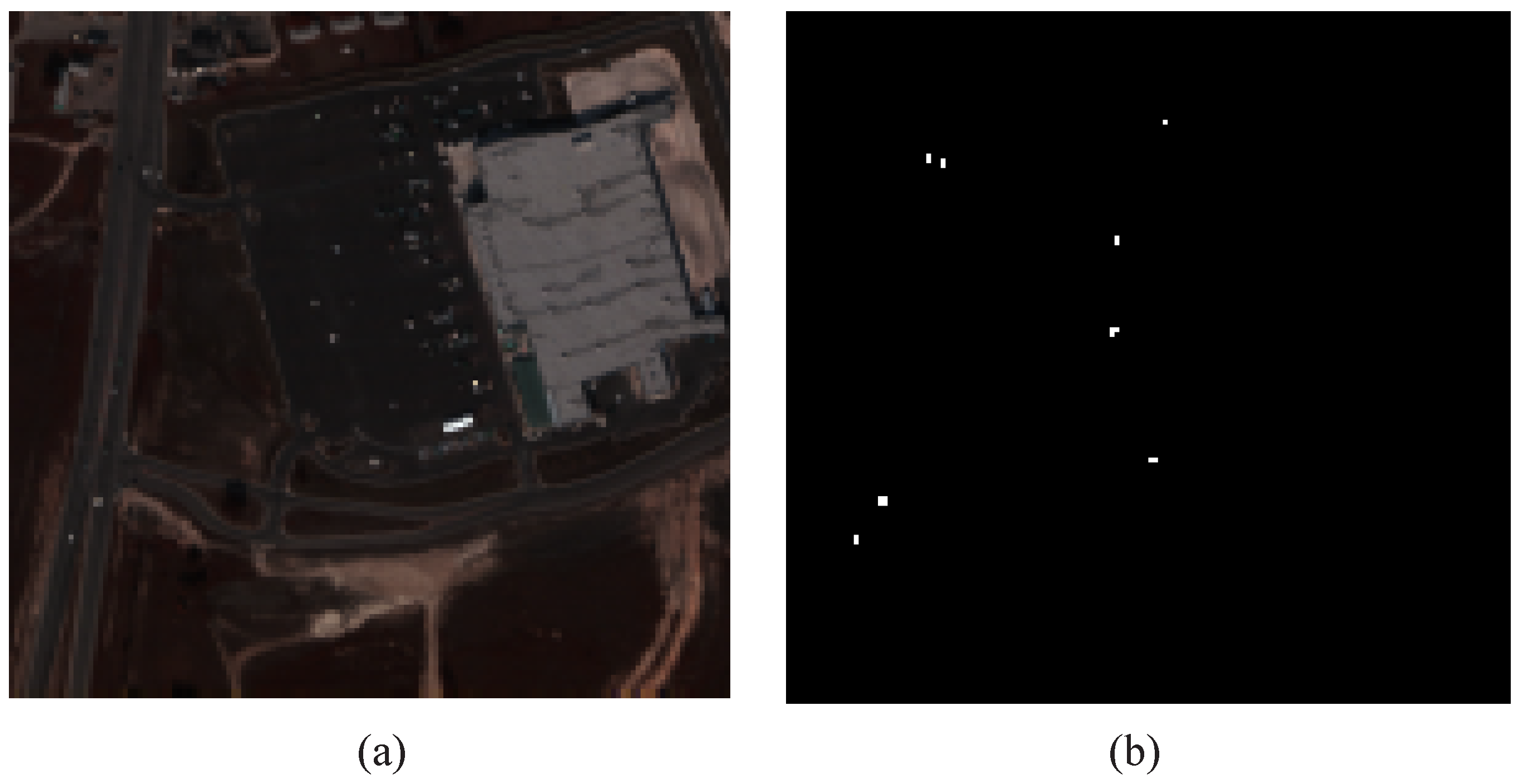
HYDICE urban dataset: The HYDICE urban dataset is widely used in hyperspectral anomaly detection and is acquired by the hyperspectral digital image acquisition experiment sensor. The original image size is $307\times 307\times 210$. After removing noise and bands affected by water absorption, 160 bands were retained. In this paper, the original images are cropped to obtain a dataset with the size of $80\times 100\times 160$. Figure 2 shows the visualization of HYDICE urban data and their corresponding ground truth.

(2)

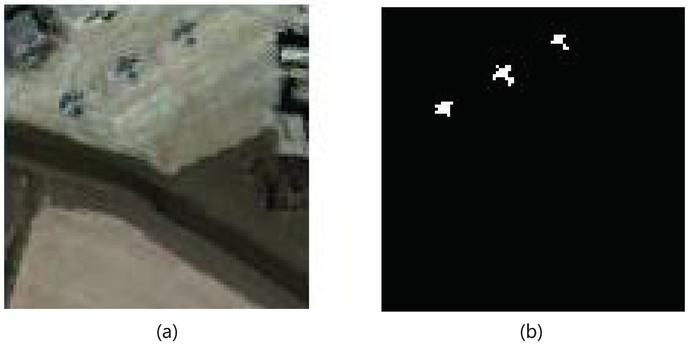
AVIRIS airplane dataset: the AVIRIS aircraft dataset is acquired from the Infrared Imaging Spectrometer in San Diego, CA, USA. The AVIRIS airplane dataset has a spatial resolution of 20 m and a spectral resolution of 10 nm, with a spectral wavelength range from 370 nm to 2510 nm. The AVIRIS aircraft dataset has a spatial size of $100\times 100$, with 224 bands. Considering the absorption region, low signal-to-noise ratio and damaged bands, 189 bands are reserved for experiments. Figure 3 illustrates the visualization of the AVIRIS airplane dataset and its corresponding ground truth.

(3)

Salinas Valley dataset: The Salinas Valley dataset captures an image of the Salinas Valley in California, USA, taken by the AVIRIS imaging spectrometer. The original image size is $512\times 217\times 224$, and the dataset is cropped to obtain dimensions of $180\times 180\times 224$. Figure 4 presents a visual display of the Salinas Valley dataset and its corresponding ground truth.

4.2. Evaluation Criteria

To conduct a comprehensive assessment of the proposed method, we employed qualitative and quantitative analyses using Receiver Operating Characteristic (ROC) curves and Area Under Curve (AUC) values. The Receiver Operating Characteristic (ROC) curve is a graphical representation that illustrates the performance of a binary classifier across various discrimination thresholds. It shows the relationship between the True Positive Rate (TPR) and the False Positive Rate (FPR) as the threshold for classification is adjusted. The FPR and TPR are defined as follows:

$$\mathrm{TPR}=\frac{\mathrm{TP}}{\mathrm{TP}+\mathrm{FN}}$$

(8)

$$\mathrm{FPR}=\frac{\mathrm{FP}}{\mathrm{FP}+\mathrm{TN}}$$

(9)

where TP represents true positive, TN is true negative, FP means false positive, and FN refers to false negative. The AUC is a widely used metric derived from the ROC curve. It quantifies the overall performance of the classifier. A higher AUC value indicates better classification accuracy, with a value of 1 indicating perfect classification.

4.3. Comparison with State-of-the-Arts

To demonstrate the effectiveness of the proposed hyperspectral anomaly detection algorithm based on the channel attention mechanism and LRX, we compared it with six existing algorithms: LRX ([7], Background of Joint Sparse Representation (BJSR) [14], LRaSMD [15], Modified Collaborative Representation Detector (MCRD) [29], Auto-Encoder-based (AE-based) [26], and Autonomous hyperspectral anomaly detection method based on full convolutional auto-encoder (AUTO-AD) [23]. The detection results of all algorithms are evaluated from both qualitative and quantitative perspectives. The brief descriptions of the six compared algorithms are described below.

(1)

The LRX algorithm is similar to the GRX algorithm. However, the LRX applies a double window sliding strategy to detect anomalies, reducing the effect of the overall background noise [30].

(2)

BJSR constructs overcomplete background dictionaries using background samples. It detects anomalies by computing the reconstruction error and estimating adaptive orthogonal background complementary subspaces [16].

(3)

LRaSMD decomposes the input image into a low-rank matrix representing the background and a sparse matrix representing the anomaly by low rank decomposition. It constructs the background and calculates the Mahalanobis distance based on the background statistics to detect anomalies [15].

(4)

MCRD uses residuals to detect anomalies by removing pixels whose spectrum are significantly different from the majority of pixels in the background, aiming to obtain more representative background pixels [31].

(5)

AE-based algorithm employs an encoder–decoder network to extract features and reconstructs the original image. Anomalies are detected by calculating the reconstruction errors [32].

(6)

AUTO-AD algorithm reconstructs the background by a fully convolutional auto-encoder with skip connections. Anomaly detection is performed by analyzing the difference between the generated map and the original image [23].

Figure 5 presents a comparison of the ROC curves between the proposed algorithm and the six comparison algorithms. From Figure 5, it can be seen that the ROC curves of the proposed algorithm are more to the upper left corner than those of the other six algorithms, surpassing the curves of the other six algorithms. This indicates that the proposed algorithm exhibits superior anomaly detection accuracy compared to the others. Specifically, in the HYDICE urban dataset and Salinas Valley dataset, the ROC curves of the proposed algorithm are significantly closer to the upper left corner than those of the other algorithms, further highlighting its better anomaly detection performance in these datasets. Although the detection performance of the proposed algorithm in the AVIRIS aircraft dataset is not as obvious as in the other two datasets, its ROC curves still outperform those of the other algorithms.

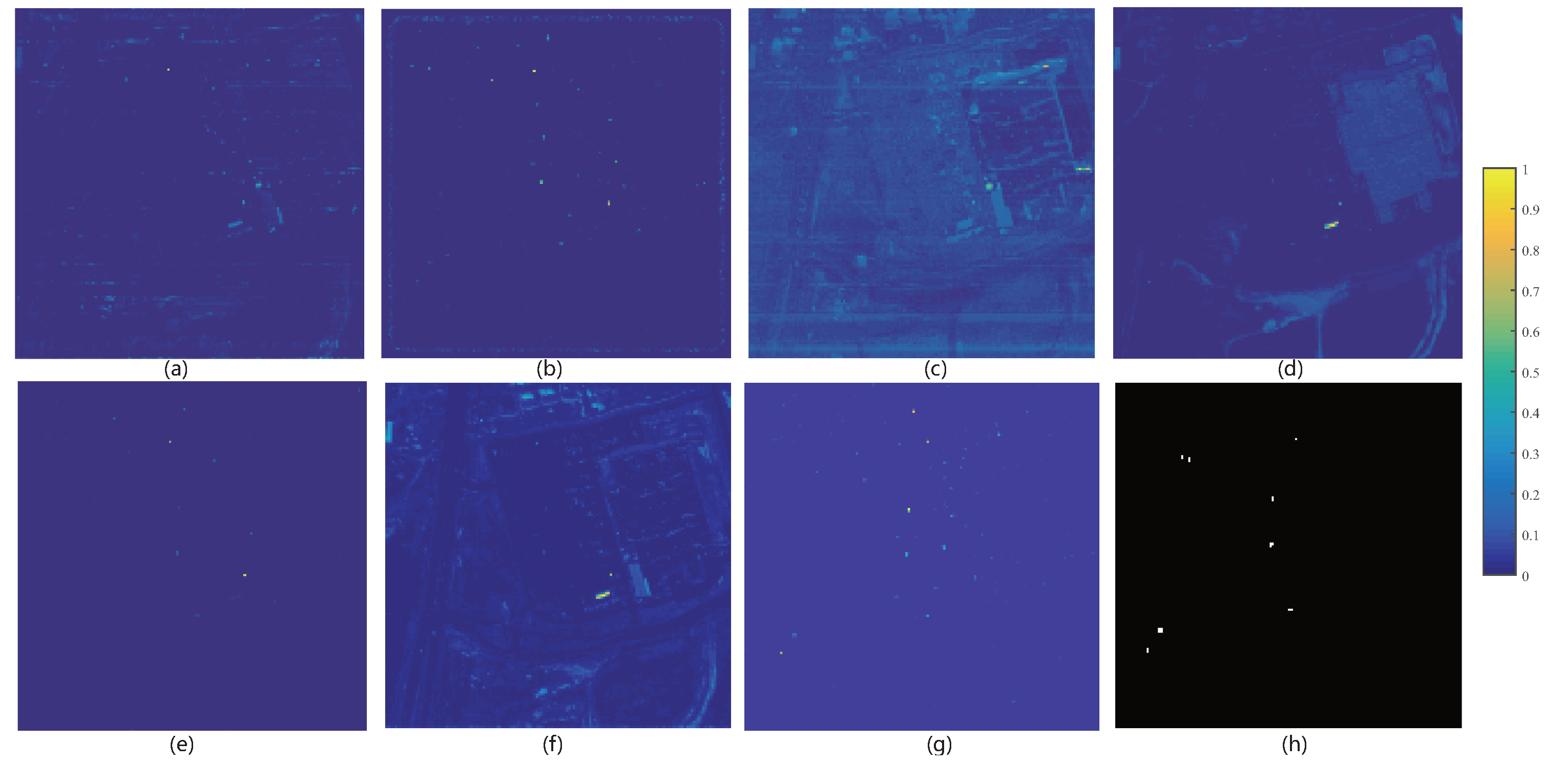
The anomaly detection results for the HYDICE urban dataset visualization are shown in Figure 6. In the visualization, pixels that are closer to yellow indicate a higher probability of being anomalous targets, while pixels closer to blue represent a higher probability of being background pixels. From Figure 6, it can be seen that the LRX, MCRD, and AUTO-AD algorithms have a high miss rate, incorrectly identifying anomalous targets as background pixels. In contrast, the BJSR-, LRaSMD-, and AE-based algorithms demonstrate a high false alarm rate, incorrectly classifying some background pixels as anomalous targets. Both the proposed algorithm and the LRX algorithm achieved better detection performance than the other compared algorithms. The proposed algorithm, which incorporates an channel attention mechanism to focus on the effective bands of different land covers during feature extraction, achieves better anomaly detection results than the LRX algorithm. By effectively reducing noise in the reconstruction image, the proposed algorithm successfully detects nearly all anomalies and demonstrates a relatively high discrimination between anomalous and background pixels.

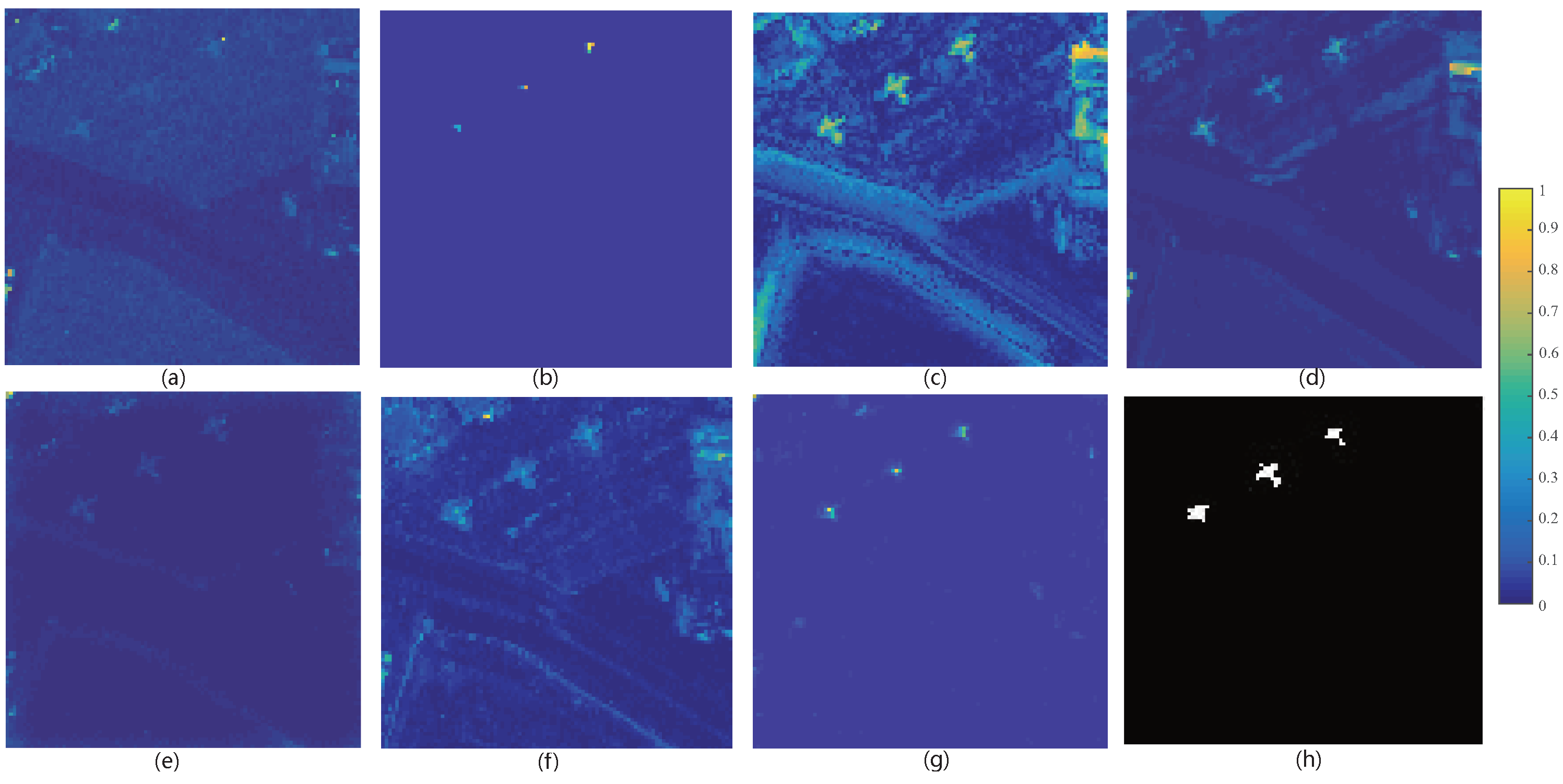
The results of anomaly detection for the visualization of the AVIRIS airplane dataset are depicted in Figure 7. LRaSMD, AE-based and AUTO-AD algorithms can detect most of the anomalies. However, these detected anomalies often have low anomaly intensity values, and there are instances where the background is incorrectly identified as anomalous. The MCRD algorithm also detects anomalies with low intensity values, making it difficult to distinguish them from the background. Additionally, some anomaly targets are incorrectly classified as background pixels. Although the BJSR algorithm detects a large number of anomalies, it detects many background pixels as anomalies by mistakes and has a high false detection rate. LRX demonstrates better detection accuracy, but it still has a certain miss detection rate and incorrectly detects anomalies as background. The proposed hyperspectral anomaly detection algorithm based on the channel attention mechanism and LRX detects anomalies with higher intensity values than the LRX algorithm. This leads to a significant reduction in the probability of missed detections.

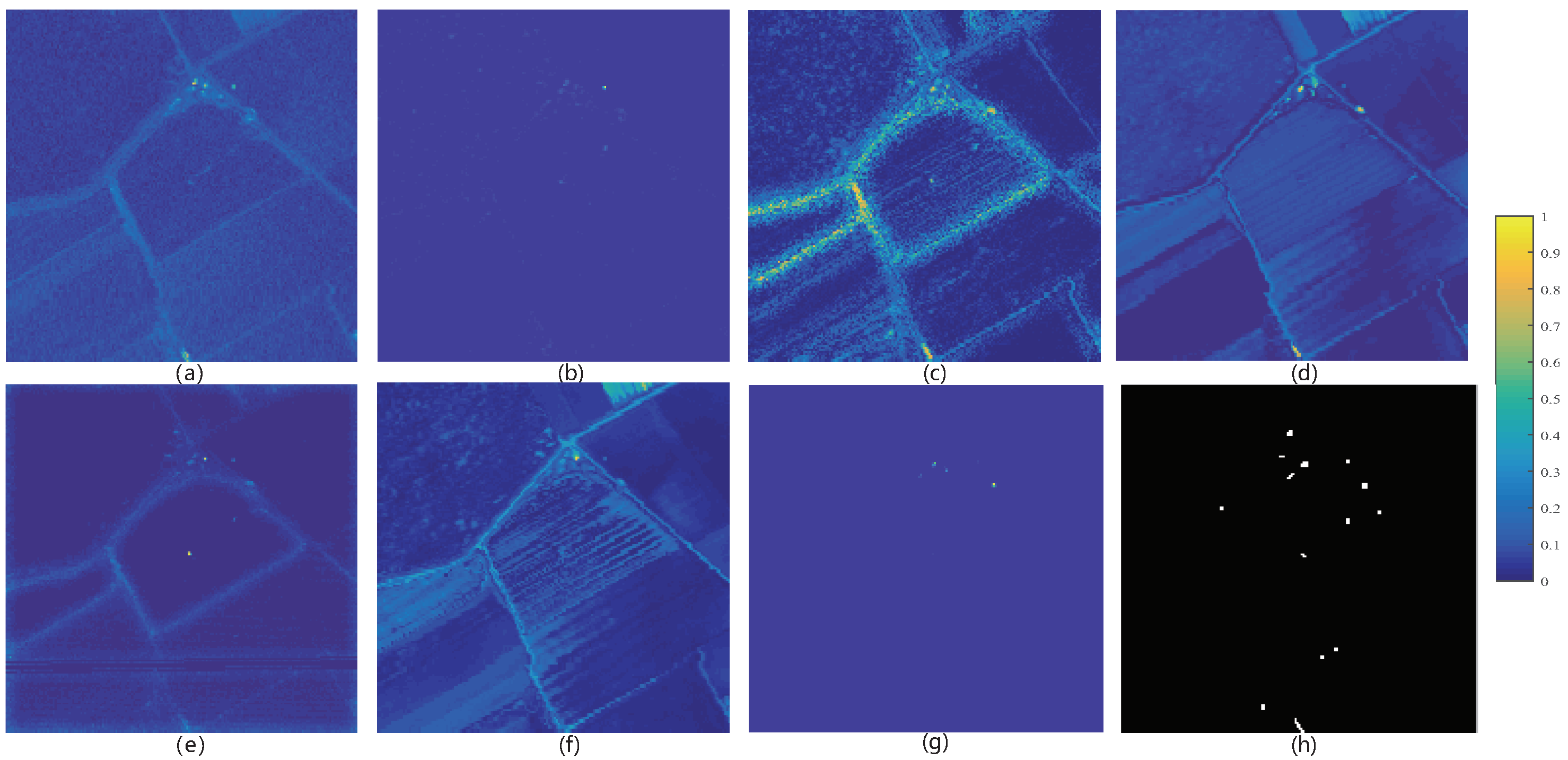
The anomaly detection results visualized for the Salinas dataset are presented in Figure 8. LRX misses most of the anomalous targets, while BJSR incorrectly identifies many background pixels as anomalous targets. LRaSMD, MCRD, AE-based, and AUTO-AD algorithms outperform LRX and BJSR in the detection accuracy. However, there are still cases of misdetection, where some background pixels are incorrectly classified as anomalous targets. The proposed method in this paper exhibits a few missed detections for some anomalous targets, but performs well in distinguishing them from the background for the majority of anomalous targets. Therefore, the proposed algorithm in this paper achieves the best detection result.

While the ROC curve provides qualitative insight into the performance of anomaly detection algorithms, it may not always clearly indicate which algorithm is superior. Therefore, quantitative analysis is necessary to facilitate better comparisons. The AUC value, which represents the area under the ROC curve, serves as an important evaluation metric. A larger AUC indicates better detection performance. The AUC values of the proposed algorithm and the six compared algorithms on the three hyperspectral datasets are presented in

Table 2. AUC values of different algorithms on the three hyperspectral data.

Method	Dataset
	HYDICE Urban	AVIRIS Airplane	Salinas Scene
LRX	$0.9737$	$0.9496$	$0.9291$
BJSR	$0.7988$	$0.981$	$0.9533$
LRaSMD	$0.779$	$0.9854$	$0.8187$
MCRD	$0.9071$	$0.9512$	$0.8972$
AE-based	$0.8871$	$0.9829$	$0.8929$
AUTO-AD	$0.9646$	$0.9764$	$0.9582$
Ours	$0.9871$	$0.9916$	$0.9642$

.

From Table 2, it can be seen that the AUC values of the proposed algorithm in this paper are higher than those of the LRX, BJSR, LRaSMD, MCRD, AE-based, and AUTO-AD algorithms, which are 0.9871, 0.9916, and 0.9642 on the HYDICE urban dataset, AVIRIS airplane dataset, and Salinas Valley dataset, respectively. Therefore, the proposed algorithm in this paper achieves the best anomaly detection performance on all three datasets. The AUC values of the AUTO-AD method are 0.9646, 0.9764, and 0.9582 for the HYDICE urban dataset, AVIRIS airplane dataset, and Salinas Valley dataset, respectively. The average running times for the AUTO-AD method for the HYDICE urban dataset, AVIRIS airplane dataset, and Salinas Valley dataset are 28.66, 38.57, and 35.97, respectively. On the other hand, the proposed method has average running times of 101.67, 78.81, and 131.97 for the corresponding datasets. The proposed method exhibits longer average running times due to the increased complexity introduced by the attention module and the time-consuming sliding window strategy employed in the LRX algorithm. Considering both the effectiveness of anomaly detection and the computational time required, the proposed method demonstrates satisfactory performance.

The proposed hyperspectral anomaly detection algorithm based on channel attention mechanism and LRX aims to explore the effective bands of different land covers through the auto-encode network based on the channel attention mechanism, which makes the extracted features more discriminative. By utilizing the reconstructed image for anomaly detection, the impact of noise on the detection performance of the LRX algorithm is reduced. Therefore, on the HYDICE urban dataset, the AUC value of the proposed algorithm is 0.9871, while the AUC value of the LRX algorithm is 0.9737. On the AVIRIS airplane dataset, the AUC value of the proposed algorithm is 0.9916, while the AUC value of the LRX algorithm is 0.9496. On the Salinas Valley dataset, the AUC value of the proposed algorithm is 0.9642, while the AUC value of the LRX algorithm is 0.9291. These results highlight a significant improvement in the performance of the proposed algorithm compared to the LRX algorithm across all three hyperspectral datasets.

5. Conclusions

In this paper, we propose a hyperspectral anomaly detection algorithm with a channel attention mechanism and LRX. The channel attention mechanism is utilized to guide the feature learning process of the auto-encoder, which aims to explore the effective bands of different land covers and make the reconstruction image more discriminative and less disturbed by noise. Then, the LRX algorithm is applied to the obtained reconstruction image from the auto-encoder network for anomaly detection on the reconstruction image in order to improve the performance of hyperspectral anomaly detection. The effectiveness of the proposed algorithm is verified on three different real datasets in this paper. Experimental results show that the proposed algorithm can obtain higher detection accuracy compared with other comparative algorithms.

References

1. Wang, W.; Zhao, B.; Feng, F.; Nan, J.; Li, C. Hierarchical Sub-Pixel Anomaly Detection Framework for Hyperspectral Imagery. Sensors 2018, 18, 3662. [Google Scholar] [CrossRef] [PubMed] [Green Version]
2. Racetin, I.; Krtalić, A. Systematic review of anomaly detection in hyperspectral remote sensing applications. Appl. Sci. 2021, 11, 4878. [Google Scholar] [CrossRef]
3. Li, Q.; Wang, F.; Wang, Y.; Zhou, C.; Chen, J.; Forson, K.; Miao, R.; Su, Y.; Zhang, J. Effect of reservoir characteristics and chemicals on filtration property of water-based drilling fluid in unconventional reservoir and mechanism disclosure. Environ. Sci. Pollut. Res. 2023, 30, 55034–55043. [Google Scholar] [CrossRef]
4. Li, Q.; Wang, F.; Wang, Y.; Bai, B.; Zhang, J.; Lili, C.; Sun, Q.; Wang, Y.; Forson, K. Adsorption behavior and mechanism analysis of siloxane thickener for CO2 fracturing fluid on shallow shale soil. J. Mol. Liq. 2023, 376, 121394. [Google Scholar] [CrossRef]
5. Li, Q.; Wu, J. Factors affecting the lower limit of the safe mud weight window for drilling operation in hydrate-bearing sediments in the Northern South China Sea. Geomech. Geophys. Geo-Energy Geo-Resour. 2022, 8, 82. [Google Scholar] [CrossRef]
6. Zhang, X.; Ma, X.; Huyan, N.; Gu, J.; Tang, X.; Jiao, L. Spectral-Difference Low-Rank Representation Learning for Hyperspectral Anomaly Detection. IEEE Trans. Geosci. Remote Sens. 2021, 59, 10364–10377. [Google Scholar] [CrossRef]
7. Molero, J.M.; Garzón, E.M.; García, I.; Plaza, A. Analysis and Optimizations of Global and Local Versions of the RX Algorithm for Anomaly Detection in Hyperspectral Data. IEEE J. Sel. Top. Appl. Earth Obs. Remote Sens. 2013, 6, 801–814. [Google Scholar] [CrossRef]
8. Dora, C.; Majumdar, J. Analysis of Versions of the RX Algorithm for Anomaly Detection in Hyperspectral Images. Curr. J. Appl. Sci. Technol. 2021, 40, 25–31. [Google Scholar] [CrossRef]
9. Hidalgo, J.A.P.; Pérez-Suay, A.; Nar, F.; Camps-Valls, G. Efficient nonlinear RX anomaly detectors. IEEE Geosci. Remote Sens. Lett. 2020, 18, 231–235. [Google Scholar] [CrossRef]
10. Kwon, H.; Nasrabadi, N.M. Kernel RX-algorithm: A nonlinear anomaly detector for hyperspectral imagery. IEEE Trans. Geosci. Remote Sens. 2005, 43, 388–397. [Google Scholar] [CrossRef]
11. Padrón-Hidalgo, J.A.; Laparra, V.; Camps-Valls, G. Unsupervised anomaly and change detection with multivariate gaussianization. IEEE Trans. Geosci. Remote Sens. 2021, 60, 1–10. [Google Scholar] [CrossRef]
12. Li, W.; Du, Q. Collaborative Representation for Hyperspectral Anomaly Detection. IEEE Trans. Geosci. Remote Sens. 2015, 53, 1463–1474. [Google Scholar] [CrossRef]
13. Wu, Z.; Su, H.; Tao, X.; Han, L.; Paoletti, M.E.; Haut, J.M.; Plaza, J.; Plaza, A. Hyperspectral Anomaly Detection With Relaxed Collaborative Representation. IEEE Trans. Geosci. Remote Sens. 2022, 60, 1–17. [Google Scholar] [CrossRef]
14. Li, J.; Zhang, H.; Zhang, L.; Ma, L. Hyperspectral Anomaly Detection by the Use of Background Joint Sparse Representation. IEEE J. Sel. Top. Appl. Earth Obs. Remote Sens. 2015, 8, 2523–2533. [Google Scholar] [CrossRef]
15. Sun, W.; Liu, C.; Li, J.; Lai, Y.M.; Li, W. Low-rank and sparse matrix decomposition-based anomaly detection for hyperspectral imagery. J. Appl. Remote Sens. 2014, 8, 083641. [Google Scholar] [CrossRef]
16. Wu, C.; Du, B.; Zhang, L. Hyperspectral anomalous change detection based on joint sparse representation. ISPRS J. Photogramm. Remote Sens. 2018, 146, 137–150. [Google Scholar] [CrossRef]
17. Ruhan, A.; Mu, X.; He, J. Enhance Tensor RPCA-Based Mahalanobis Distance Method for Hyperspectral Anomaly Detection. IEEE Geosci. Remote Sens. Lett. 2022, 19, 1–5. [Google Scholar]
18. Zhang, L.; Cheng, B. Transferred CNN Based on Tensor for Hyperspectral Anomaly Detection. IEEE Geosci. Remote Sens. Lett. 2020, 17, 2115–2119. [Google Scholar] [CrossRef]
19. Arisoy, S.; Nasrabadi, N.M.; Kayabol, K. GAN-based Hyperspectral Anomaly Detection. In Proceedings of the 2020 28th European Signal Processing Conference (EUSIPCO), Amsterdam, The Netherlands, 18–21 January 2021; pp. 1891–1895. [Google Scholar] [CrossRef]
20. Zhao, C.; Li, X.; Zhu, H. Hyperspectral anomaly detection based on stacked denoising autoencoders. J. Appl. Remote Sens. 2017, 11, 042605. [Google Scholar] [CrossRef]
21. Zhao, Z.; Sun, B. Hyperspectral anomaly detection via memory-augmented autoencoders. CAAI Trans. Intell. Technol. 2022, 1–14. [Google Scholar] [CrossRef]
22. Shi, C.; Liao, D.; Zhang, T.; Wang, L. Hyperspectral Image Classification Based on 3D Coordination Attention Mechanism Network. Remote Sens. 2022, 14, 608. [Google Scholar] [CrossRef]
23. Wang, S.; Wang, X.; Zhang, L.; Zhong, Y. Auto-AD: Autonomous Hyperspectral Anomaly Detection Network Based on Fully Convolutional Autoencoder. IEEE Trans. Geosci. Remote Sens. 2022, 60, 1–14. [Google Scholar] [CrossRef]
24. Lu, X.; Zhang, W.; Huang, J. Exploiting Embedding Manifold of Autoencoders for Hyperspectral Anomaly Detection. IEEE Trans. Geosci. Remote Sens. 2020, 58, 1527–1537. [Google Scholar] [CrossRef]
25. Xie, W.; Liu, B.; Li, Y.; Lei, J.; Du, Q. Autoencoder and Adversarial-Learning-Based Semisupervised Background Estimation for Hyperspectral Anomaly Detection. IEEE Trans. Geosci. Remote Sens. 2020, 58, 5416–5427. [Google Scholar] [CrossRef]
26. Bati, E.; Çalışkan, A.; Koz, A.; Alatan, A.A. Hyperspectral anomaly detection method based on auto-encoder. In Proceedings of the Image and Signal Processing for Remote Sensing XXI, Toulouse, France, 21–23 September 2015; Bruzzone, L., Ed.; International Society for Optics and Photonics, SPIE: Bellingham, WA, USA, 2015; Volume 9643, p. 96430N. [Google Scholar] [CrossRef]
27. Guo, R.; Xiao, P.; Zhang, X.; Liu, H. Updating land cover map based on change detection of high-resolution remote sensing images. J. Appl. Remote Sens. 2021, 15, 044507. [Google Scholar] [CrossRef]
28. Li, X.; Zhao, C.; Yang, Y. Hyperspectral anomaly detection based on the distinguishing features of a redundant difference-value network. Int. J. Remote Sens. 2021, 42, 5455–5473. [Google Scholar] [CrossRef]
29. Vafadar, M.; Ghassemian, H. Anomaly Detection of Hyperspectral Imagery Using Modified Collaborative Representation. IEEE Geosci. Remote Sens. Lett. 2018, 15, 577–581. [Google Scholar] [CrossRef]
30. Küçük, S.; Yüksel, S.E. Comparison of RX-based anomaly detectors on synthetic and real hyperspectral data. In Proceedings of the 2015 7th Workshop on Hyperspectral Image and Signal Processing: Evolution in Remote Sensing (WHISPERS), Tokyo, Japan, 2–5 June 2015; pp. 1–4. [Google Scholar] [CrossRef]
31. Ma, N.; Peng, Y.; Wang, S. A Fast Recursive Collaboration Representation Anomaly Detector for Hyperspectral Image. IEEE Geosci. Remote Sens. Lett. 2019, 16, 588–592. [Google Scholar] [CrossRef]
32. Xie, W.; Lei, J.; Liu, B.; Li, Y.; Jia, X. Spectral constraint adversarial autoencoders approach to feature representation in hyperspectral anomaly detection. Neural Netw. 2019, 119, 222–234. [Google Scholar] [CrossRef]
Figure 1. Network structure of the proposed hyperspectral anomaly detection algorithm based on the channel attention mechanism and LRX.
Applsci 13 06988 g001
Figure 2. (a) The pseudo-color image of HYDICE urban dataset. (b) The ground truth.
Applsci 13 06988 g002
Figure 3. (a) The pseudo-color image of AVIRIS airplane dataset. (b) The ground truth.
Applsci 13 06988 g003
Figure 4. (a) The pseudo-color image of Salinas Valley dataset. (b) The ground truth.
Applsci 13 06988 g004
Figure 5. ROC curves of six comparative algorithms and the proposed algorithm on three data sets: (a) HYDICE urban data; (b) AVIRIS airplane data; (c) Salinas scene.
Applsci 13 06988 g005
Figure 6. Visualized anomaly detection results of different algorithms on the HYDICE urban dataset: (a) LRX; (b) BJSR; (c) LRaSMD; (d) MCRD; (e) AE-based; (f) AUTO-AD; (g) ours; (h) ground truth.
Applsci 13 06988 g006
Figure 7. Visualized anomaly detection results of different algorithms on AVIRIS airplane data set: (a) LRX; (b) BJSR; (c) LRaSMD; (d) MCRD; (e) AE-based; (f) AUTO-AD; (g) ours; (h) ground truth.
Applsci 13 06988 g007
Figure 8. Visualized anomaly detection results of different algorithms on Salinas Valley data set: (a) LRX; (b) BJSR; (c) LRaSMD; (d) MCRD; (e) AE-based; (f) AUTO-AD; (g) ours; (h) ground truth.
Applsci 13 06988 g008