Abstract
As an important component of intelligent transportation-management systems, accurate traffic-parameter prediction can help traffic-management departments to conduct effective traffic management. Due to the nonlinearity, complexity, and dynamism of highway-traffic data, traffic-flow prediction is still a challenging issue. Currently, most spatial–temporal traffic-flow-prediction models adopt fixed-structure time convolutional and graph convolutional models, which lack the ability to capture the dynamic characteristics of traffic flow. To address this issue, this paper proposes a spatial–temporal prediction model that can capture the dynamic spatial–temporal characteristics of traffic flow, named the spatial–temporal self-attention graph convolutional network (STA-GCN). In terms of feature engineering, we used the time cosine decomposition and one-hot encoding methods to capture the periodicity and heterogeneity of traffic-flow changes. Additionally, in order to build the model, self-attention mechanisms were incorporated into the spatial–temporal convolution to capture the spatial–temporal dynamic characteristics of traffic flow. The experimental results indicate that the performance of the proposed model on two traffic-volume datasets is superior to those of several baseline models. In particular, in long-term prediction, the prediction error can be reduced by over 5%. Further, the interpretability and robustness of the prediction model are addressed by considering the spatial dynamic changes.
1. Introduction
Traffic congestion has become a serious problem due to the development of the economy and the dramatic increase in vehicles on the road, which has also resulted in environmental pollution and low traffic efficiency [1]. The timely prediction of traffic parameters, such as traffic volume, speed, and occupancy, is believed to effectively improve road capacity, alleviate traffic congestion, provide traffic-route information for urban travelers, and help traffic authorities to make better decisions. Traffic-flow prediction is still an important component within intelligent transportation systems (ITS).
In the past decade, extensive of studies on traffic-flow prediction have been conducted, which can be divided into two categories: model-driven and data-driven approaches. The model-driven methods were introduced to simulate traffic problems in terms of important parameters. However, the assumptions made for the model were usually not suitable for real-world traffic conditions [2]. On the other hand, through the development of traffic detectors and big-data-mining techniques, data-driven methods have gradually become a major research topic.
Generally, statistical models and classical machine-learning models were first used for traffic-flow prediction at a single traffic node. Statistical models, involving ARIMA and its variants [3,4], were restricted by the assumption of stationary time series, which led to poor performance in predicting non-linear changes in traffic flow. Consequently, traditional machine-learning and deep-learning algorithms, such as KNN [5], SVR [6], XGBOOST [7], and LSTM [8], were proposed to capture the complex non-linear temporal changes for a single traffic node or section. However, the daily periodicity of traffic-flow changes in the time dimension and the heterogeneity of traffic-flow changes on weekdays and weekends are always ignored when feature engineering is conducted. Moreover, to construct the prediction model in a complex traffic network, it is necessary to establish a prediction model for each station without considering the spatial correlation.
In order to capture the spatial correlation in a traffic-flow-prediction model, many scholars define the traffic network through a regular grid space in terms of CNN [9,10,11]. However, the topological information between irregular traffic network nodes is often ignored. With the emergence of graph neural networks (GNN), deep learning has been extended to non-Euclidean fields [12], and the subsequent graph convolutional neural network has become an effective model for demonstrating the spatial dependence of traffic networks [13]. Yu et al. [14] used graph convolutional neural networks and gated convolutional neural networks to construct the STGCN model, which achieved good prediction results in real traffic scenarios. However, the fixed spatial topological structure and a convolution structure that fused an adjacent time-stamp as prediction information could not effectively capture dynamic spatial–temporal characteristics. To solve this issue, Guo et al. [15] proposed a graph convolutional network (GCN) based on a spatial–temporal attention mechanism without considering the heterogeneity of different time periods and spatial–temporal dynamic features.
The integration of graph convolutional networks within traffic-flow-prediction models is a current research topic, which aims to capture the dynamic spatiotemporal patterns of traffic flow and consider the periodic heterogeneity of traffic flow in the temporal dimension. Therefore, to address concerns over the current spatial–temporal traffic-flow-prediction models, in this paper, we propose methods involving the periodic characteristics of traffic flow and dynamic spatial–temporal dependence. Specifically, the periodic characteristics of traffic flow in daily changes and the heterogeneity of weekdays and weekends were considered during feature encoding, which were utilized as the input variables for traffic-flow prediction. In addition, a self-attention mechanism was introduced to capture the dynamic dependence of traffic flow on both the temporal and spatial dimensions. Furthermore, the gated mechanism was utilized to selectively extract the important features to further improve the prediction performance.
2. Literature Review
As mentioned above traffic-flow prediction providing typical time-series prediction is one of the essential parts of ITS, which is still a challenging issue. Over the past decades, various models and techniques were employed in traffic-flow prediction, which can be roughly divided into model-driven and data-driven approaches [16,17].
The model-driven approaches mainly depend on mathematical statistics or historical observations in constructing parametric models, which include time-series models, Kalman filtering models, spectral analyses, etc. Many classic models are proposed for traffic-flow prediction, such as the autoregression moving-average model (ARMA) and autoregression integral moving-average model (ARIMA) [18,19]. However, parametric models, which are easily affected by external environmental factors, do not effectively deal with the non-linear issue of traffic. Compared to model-driven methods, data-driven methods mainly focus on the relationship between input and output rather than the model parameters. Example models include SVR, Kalman filtering, and artificial neural networks (ANNs) [20], which clearly illustrate non-linear mapping capability for prediction and weakness in learning the spatio-temporal characteristics of network traffic flow.
Recently, the data-driven models of traffic-flow prediction have shifted to deep-learning methods in terms of the temporal and spatial features. For instance, the graph convolutional network (GCN) extends convolutional operations from structured data to graph-structured data, mainly through spatial domain convolutions [21] and spectral domain convolutions [22]. Regarding spatial domain convolutions, Li et al. [23] modeled traffic flow as a diffusion process on a directed graph and proposed the diffusion convolutional recurrent neural network (DCRNN), which captures spatial correlations based on bidirectional random walks to predict traffic flow on large road networks. Song et al. [24] added spatial–temporal correlations between adjacent matrices of a graph and constructed a prediction framework using a combination of spatial domain convolutional layers and gated linear units. Wu et al. [25] argued that explicit graph structures are not sufficient to represent node relationships in real-world graphs and proposed the Graph WaveNet architecture based on node-embedding learning. The graph convolutional layer in this architecture extracts structural features between nodes through spatial domain convolutions. Regarding spectral domain convolutions, Bruna et al. [26] proposed a general graph convolutional framework based on the graph Laplacian matrix, and Defferrard et al. [27] optimized this method using Chebyshev polynomials to approximate feature decomposition. Diao et al. [28] designed a dynamic Laplacian matrix that incorporates tensor decomposition to better capture spatial–temporal changes, and constructed a corresponding dynamic spatial–temporal graph convolutional neural network (DGCNN).
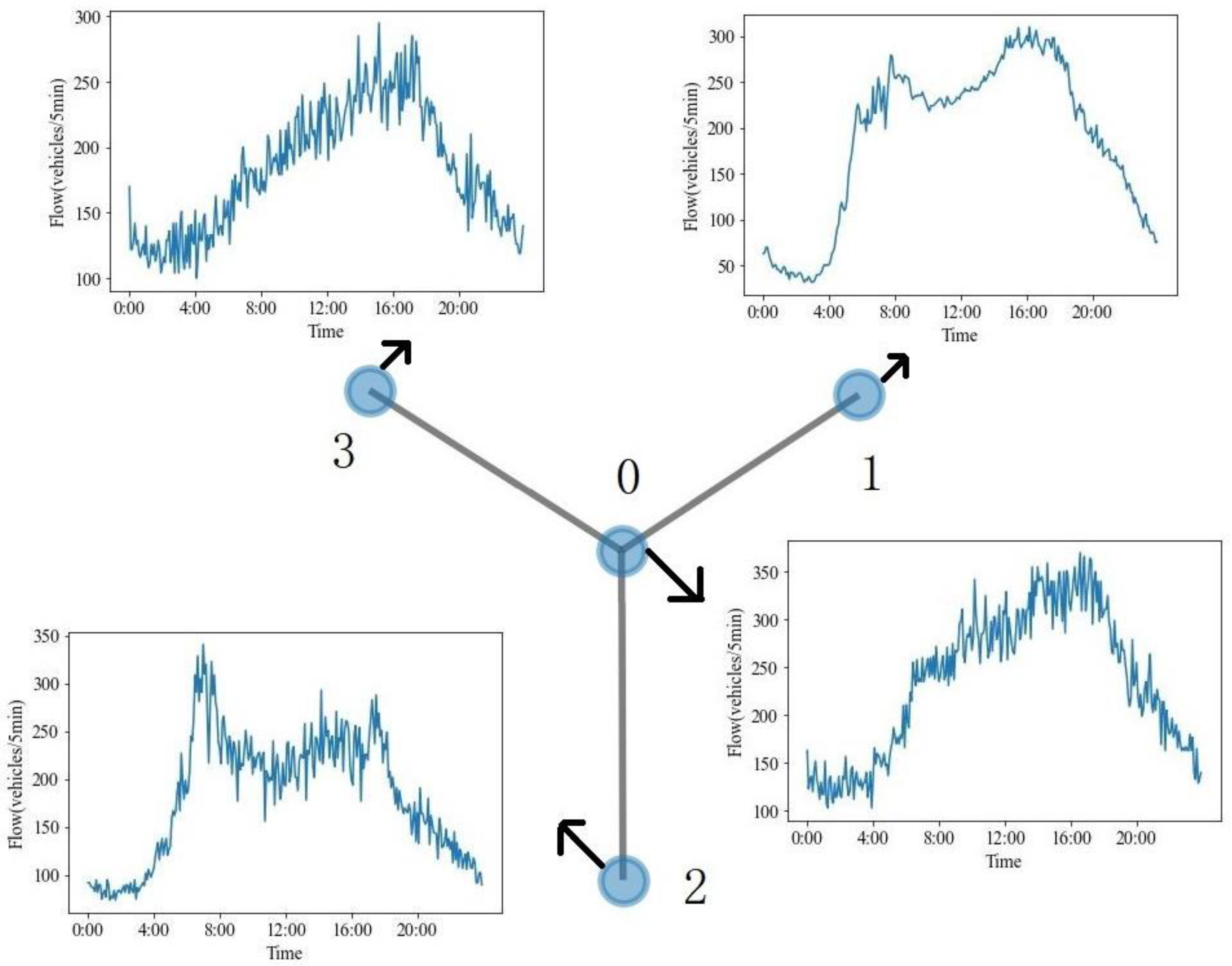
On the other hand, the Transformer model [29], proposed in 2017, is a novel foundational model that holds equal importance to CNN and RNN. In recent years, the Transformer model has made significant progress in both NLP and CV fields, and its core algorithm, the self-attention mechanism, has been widely developed and applied. Velickovic et al. [30] used self-attention layers to process graph-structured data through neural networks and achieved state-of-the-art results. Cai et al. [31] used Transformer to capture temporal correlations in traffic flow and combined these with GNN, which can capture spatial dependencies, to build a spatial–temporal traffic-flow prediction model. Xu et al. [32] used a self-attention mechanism to simultaneously capture spatial and temporal dependencies of traffic-state changes, but when capturing spatial dependencies, the computational cost was excessively high due to the large number of spatial nodes. In real traffic scenarios, due to factors such as road characteristics and PIO types, although two nodes are adjacent, there may be differences in traffic state in the same time period, as shown in Figure 1.
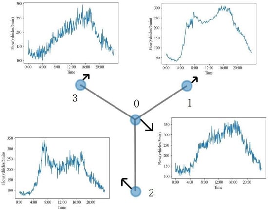
Figure 1.
Various trends in daily traffic volume for adjacent network nodes.
Nodes 1, 2, and 3 are adjacent to node 0, but each node has different traffic trends and peak periods. The results indicate heterogeneity in traffic-state changes among adjacent traffic nodes during the same time period. Therefore, a fixed-graph structure is not sufficient to capture complex dynamic traffic-flow changes. In this study, a spatial self-attention mechanism was used to capture the dynamic changes in traffic flow in the spatial dimension. Subsequently, two different attention forms were used to capture the spatial–temporal dynamic features, namely a time self-attention mechanism, which considers the entire sequence for temporal dependency relationships, and a spatial attention mechanism, for road-network-traffic-node spatial characteristics.
3. Dataset and Methodology
3.1. Dataset
Two publicly available datasets from real world are utilized in this study. (1) PeMSD04, which contains traffic-flow data from the San Francisco Bay Area. The dataset includes 340 sensors, and the selected experimental period covers two months, from 1 January 2018 to 28 February 2018. (2) PeMSD08, a real-time traffic-flow-sensor data set, includes data from 295 sensor detectors from a two-month experiment period from 1 July 2016 to 31 August 2017. The datasets were collected by the Caltrans Performance Measurement System (PeMS) [33].
3.2. Symbols and Feature Encoding
In this section, we introduce some necessary symbols and definitions that are used in this article. Next, we provide some relevant knowledge about the theoretical traffic-flow-prediction model in this article. Table 1 summarizes the main symbols.

Table 1.
Symbols.
In order to reflect the daily periodicity of traffic-flow changes in the training dataset, the method of cosine decomposition [34] was used to map the daily periodicity features to two dimensions separately, as shown in Equations (1) and (2). The heterogeneity of traffic conditions between working days and weekends was differentiated by using one-hot encoding, with weekends coded as 0 and working days coded as 1. As a result, the input data had 4 channels: traffic speed, time sine component, time cosine component, and heterogeneity components for working days and weekends.
The and are the sequences of cosine and sine components, respectively, for a time series. The is the length of the period, and is a set of integer sequences starting from 0.
3.3. Spatial–Temporal Self-Attention Graph Convolution Networks (STA-GCN)
In this section, the detailed description of the STA-GCN (spatial–temporal self-attention graph convolution network) model structure is provided. As shown in Figure 2, the model consists of an input layer, an output layer, and a spatial–temporal layer. The input layer is a fully connected neural network that maps the input spatial–temporal information , which is encoded with time, from 4 channels to a higher-dimensional channel. The spatial–temporal layer is composed of a temporal layer and a spatial layer, and we describe the model structures of these two layers in detail below.
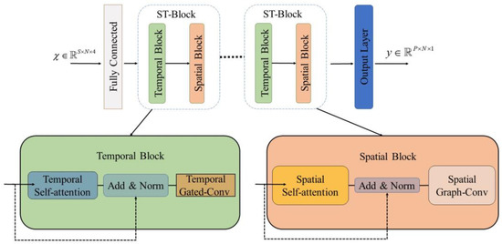
Figure 2.
Structure diagram of STA-GCN model.
3.3.1. Temporal Self-Attention
The self-attention mechanism is the core algorithm of the Transformer model, which can capture the dependency relationship between sequences through the query matrix Q, key matrix K, and value matrix V. Similarly, the dependency relationship between traffic-flow features at different time steps can be captured by the self-attention mechanism. The formula for calculating the temporal self-attention is shown in Equation (3).
The , , and refer to the time-series query matrix, key matrix, and value matrix, respectively. These matrices are used in the self-attention mechanism to capture the dependency relationship between traffic-flow features at different time steps. The query matrix A contains the queries that are compared with the keys in the key matrix B, and the value matrix C contains the values corresponding to the keys. The softmax function performs a normalization operation on the temporal dependencies at each time step. The scaling factor is applied to prevent significant differences in the probability distribution of the matrix resulting from the dot product of points and after passing through the softmax function. After obtaining the attention-probability matrix, a linear layer is applied to obtain , which is then residually connected with and normalized along the dimension. Finally, the output is passed through a ReLu activation function.
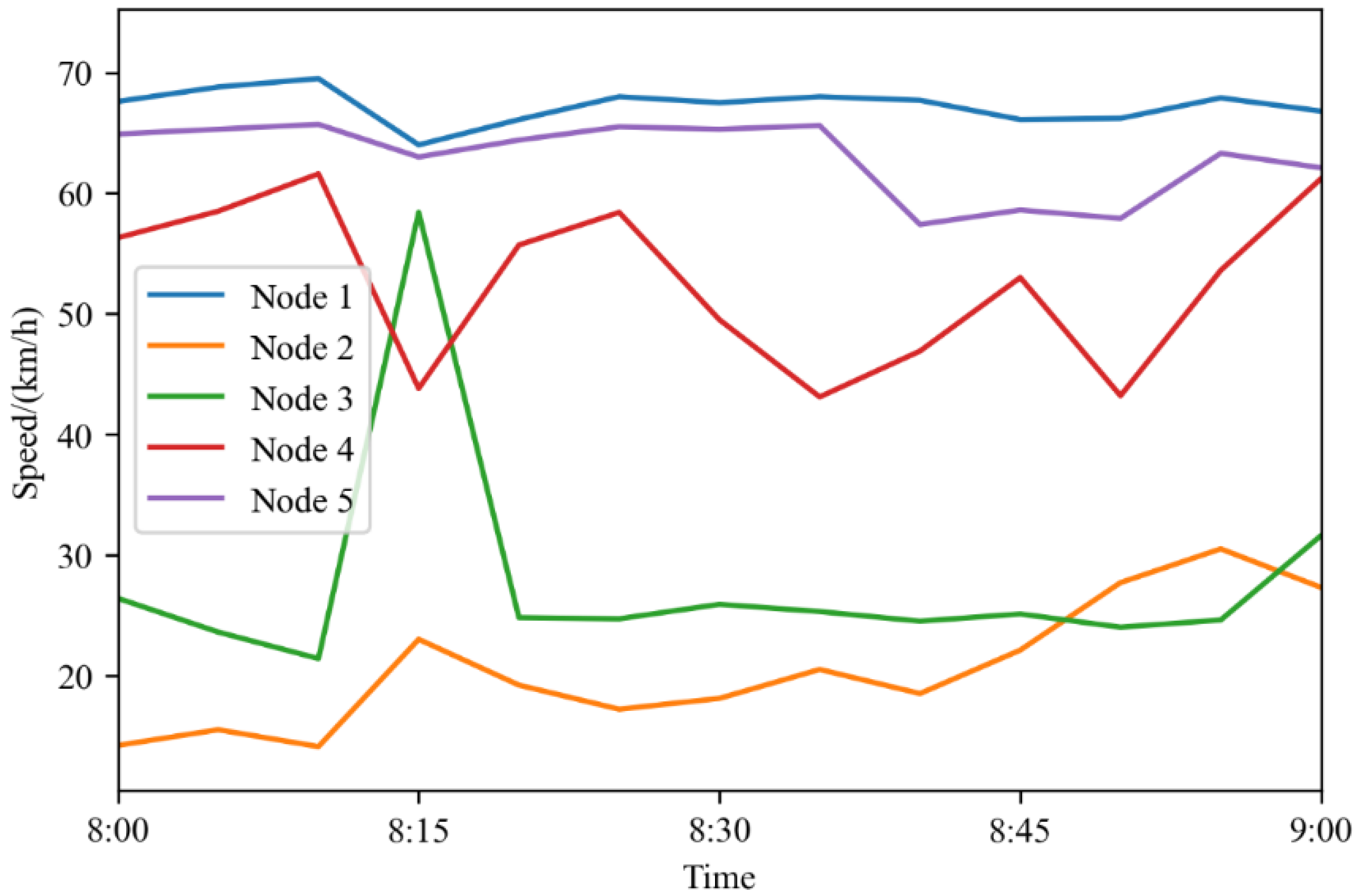
Due to the different geographical locations of transportation nodes, different transportation nodes exhibit different traffic conditions during a certain time period. As shown in Figure 3, there is a significant difference in the traffic-speed changes of the five transportation nodes during the time period from 8:00 to 9:00, indicating the existence of heterogeneity in spatial traffic characteristics. Therefore, it is necessary to capture the time-varying dependence relationship for each transportation node. As shown in Figure 4, the spatial–temporal information from multiple transportation nodes is summed up after passing through a time-attention mechanism, forming an input to the temporal gated convolution.
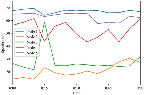
Figure 3.
Traffic-speed variation at different transportation nodes during the same period.
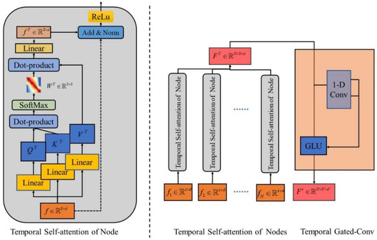
Figure 4.
Temporal module structure.
3.3.2. Temporal Gated Convolution
Although the RNN model is widely used for time-series prediction, the computational complexity of this recurrent neural network structure is relatively high. In contrast, CNNs have the advantages of fast training speed, simple structure, and no dependency constraints. Therefore, we introduced gated temporal convolution [35], and used an appropriate dilation rate for dilated convolution to obtain richer temporal dynamic correlations along the time axis. The structure of the gated temporal convolution is shown in Figure 4. After is passed through a 1D convolution layer, it is divided into two parts, and is obtained through the GLU activation function, as shown in Equation (4).
where and are two one-dimensional convolution operations. The and represent the tanh and sigmoid functions, respectively. The symbol represents the element-wise multiplication.
3.3.3. Spatial Self-Attention
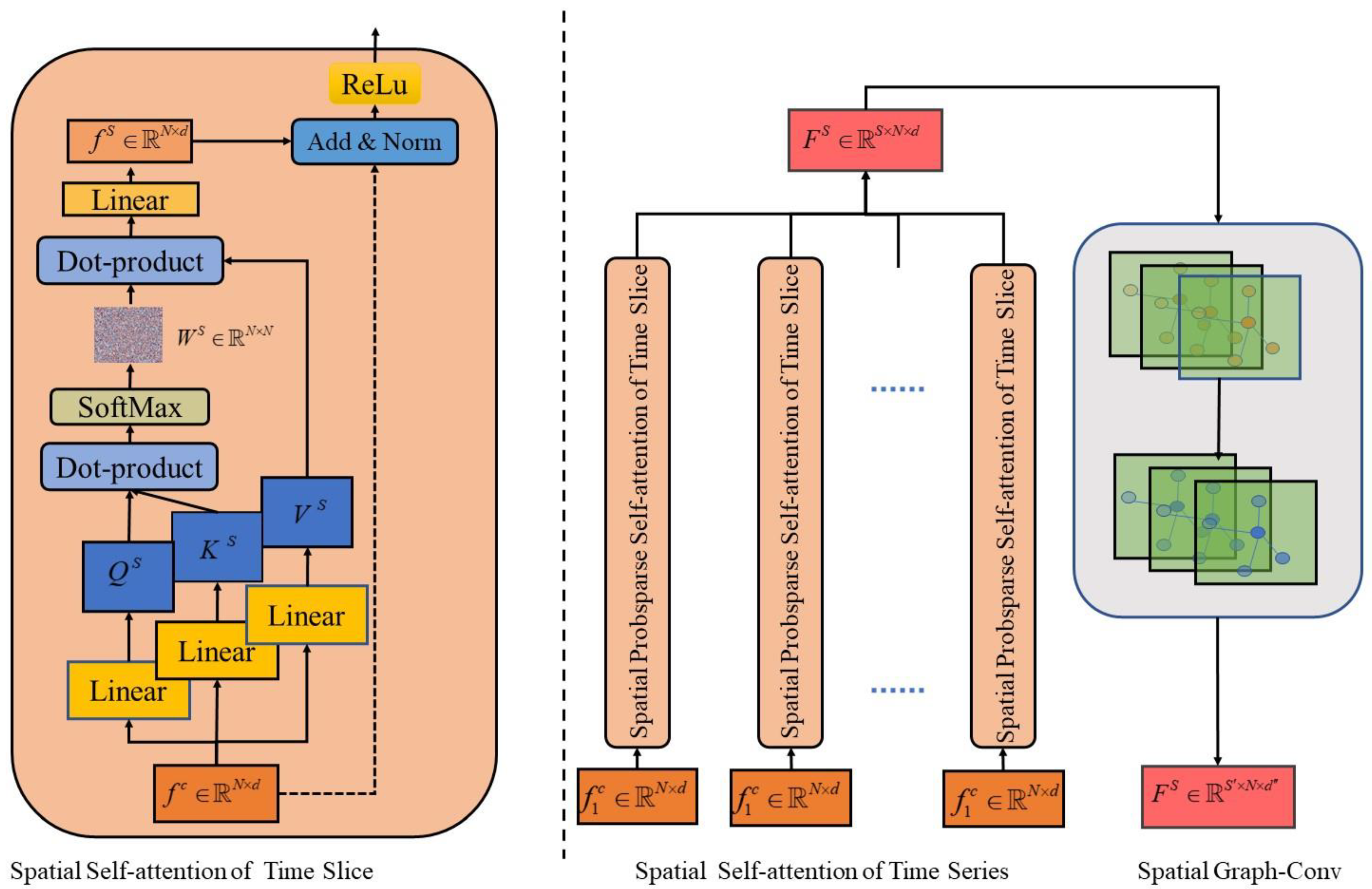
Since the spatial–temporal information output from the time module has already undergone convolution on the time axis, each vector in the time dimension can represent the spatial–temporal information of a convolution-length-time segment. The dependency relationship between each traffic node for each time segment can also be captured through self-attention mechanism. The formula for computing spatial self-attention is shown in Equation (5).
where , , and refer to the time-series query matrix, key matrix, and value matrix, respectively. These matrices are used in the self-attention mechanism to capture the dependency relationship between traffic-flow features at different time steps. The query matrix A contains the queries that are compared with the keys in the key matrix B, and the value matrix C contains the values corresponding to the keys. The softmax function performs a normalization operation on the temporal dependencies at each time step. The scaling factor is applied to prevent significant differences in the probability distribution of the matrix resulting from the dot product of points and after passing through the softmax function. After obtaining the attention-probability matrix, a linear layer is applied to obtain , which is then residually connected with and normalized along the dimension. Finally, the output is passed through a ReLu activation function.
3.3.4. Spatial Graph Convolution
The graph convolutional network (GCN) extends the convolution operation for structured data to graph-structured data. In order to fully utilize the topological relationships between various transportation nodes, spectral graph convolution is used to handle spatial dimension correlations. By analyzing the Laplacian matrix and its eigenvalues, the structural properties of the graph can be obtained. The Laplacian matrix of the graph is represented as , and in standard form as , where is the adjacency matrix, is the identity matrix, is the degree matrix, is the eigenvalue decomposition of Laplacian matrix, is a diagonal matrix, and is the Fourier basis.
The traffic parameters at time and their information on graph are represented as . The Fourier transform of this information is defined as . Graph convolution is a convolution operation that can be implemented by replacing the classic convolution operator with a diagonalizable linear operator in the Fourier domain. The formula for the convolution operation of on the graph is shown in Equation (6).
Due to the computational complexity caused by all eigenvalues and eigenvectors of the Laplacian matrix in the training process of spectral convolutional networks, this study uses graph convolutional networks based on Chebyshev polynomials to accelerate the solution of the feature matrix. The Chebyshev polynomial, as shown in Equation (7), is used for this purpose.
where is the Chebyshev segment coefficient vector, is the -th order Chebyshev polynomial of , and in , is the largest eigenvalue.
For the -th-order Chebyshev polynomial, there is a , which has a recurrence relation with the first two terms, and . The convolution operation conducted after approximating the Chebyshev polynomial shown in Equation (8) is depicted in Figure 5.

Figure 5.
Spatial module structure.
4. Results and Discussion
4.1. Data Pre-Processing
For the two datasets, we collected traffic parameters into time windows of 5 min and normalized them. We used 60% of the data as the training set, 20% as the validation set, and 20% as the test set. We use the threshold Gaussian method to establish an adjacency matrix and calculated the weights A between each detector according to Equation (9).
where represents the distance between detector and detector . The and , setting 10 and 0.5 respectively, represent the sparsity and distribution.
4.2. Parameter Setting
In this study, the STA-GCN model was implemented using the PyTorch framework, with the following parameter settings during training: a batch size of 32, the Adam optimizer, RMSE as the loss function, and an initial learning rate of 0.001.
The output dimension of the input layer was set to 32, and a (3,1) kernel was chosen for the temporal convolution based on previous work.
The Chebyshev polynomial in the graph convolution layer was set to 3.
The number of temporal and spatial modules was set to 2, and the model used the previous 12 time windows to predict the next 12 time windows. To prevent overfitting, the model stopped training if the validation loss did not decrease within 10 epochs.
4.3. Baseline Models
We compared our model to other baseline models trained on the same computer, including:
ARIMA: a classic algorithm for time-series analysis and forecasting that uses an autoregressive integrated moving-average approach.
SVR: a machine-learning algorithm that can capture non-linear temporal features.
FNN: a feedforward neural network that uses multiple hidden layers to capture non-linear temporal changes.
GRU: a type of RNN model with gated recurrent units.
FC-LSTM: a recurrent neural network with fully connected LSTM hidden units.
STGCN: a spatial–temporal traffic-flow prediction model that combines gated temporal convolutional networks with graph convolutional networks.
ASTGCN: a spatial–temporal traffic-flow prediction model that incorporates attention mechanisms to capture temporal and spatial changes. The difference between our model and ASTGCN is that ASTGCN extracts both temporal and spatial features from attention mechanisms and inputs them into spatial–temporal convolutional layers, while our model uses self-attention mechanisms to capture spatial–temporal dynamic dependencies, which are input into graph convolutional networks. Therefore, the embedding of spatial–temporal attention mechanisms is different, and our model uses self-attention mechanisms, which can capture higher-dimensional spatial–temporal dynamic characteristics.
4.4. Experimental Results
We compared our model with seven baseline models regarding the performances of different prediction horizons in Table 2, and the AST-GCN showed the best performance on both datasets. Specifically, the traditional time-series prediction methods (ARIMA, SVR) performed well on short horizons (15 min), but struggled with longer horizons (30 min, 60 min), indicating that these methods have difficulty in handling complex nonlinear traffic-flow data. Among the deep-learning models, FC-LSTM, which considers spatial dependence, and the models containing GCN modules outperformed the traditional deep-learning models (FNN and GRU). Although FC-LSTM can capture spatial features, it does not utilize the topological structure of the road network and has a significant amount of data redundancy during training. Therefore, FC-LSTM is inferior to STGCN, ASTGCN, and STA-GCN. The prediction performances of ASTGCN and STA-GCN were better than those of STGCN, demonstrating the effectiveness of adding spatial–temporal attention mechanisms to capture dynamic spatial–temporal features. Furthermore, our STA-GCN outperformed ASTGCN, especially on 60-minute horizons, with the prediction errors were reduced by 4.63% and 3.12% on the PeMSD04 and PeMSD08 datasets, respectively. These results demonstrate the superiority of the hierarchical embedding of spatial–temporal attention and the superiority of spatial–temporal self-attention mechanisms.

Table 2.
Performances of traffic-flow-prediction models.
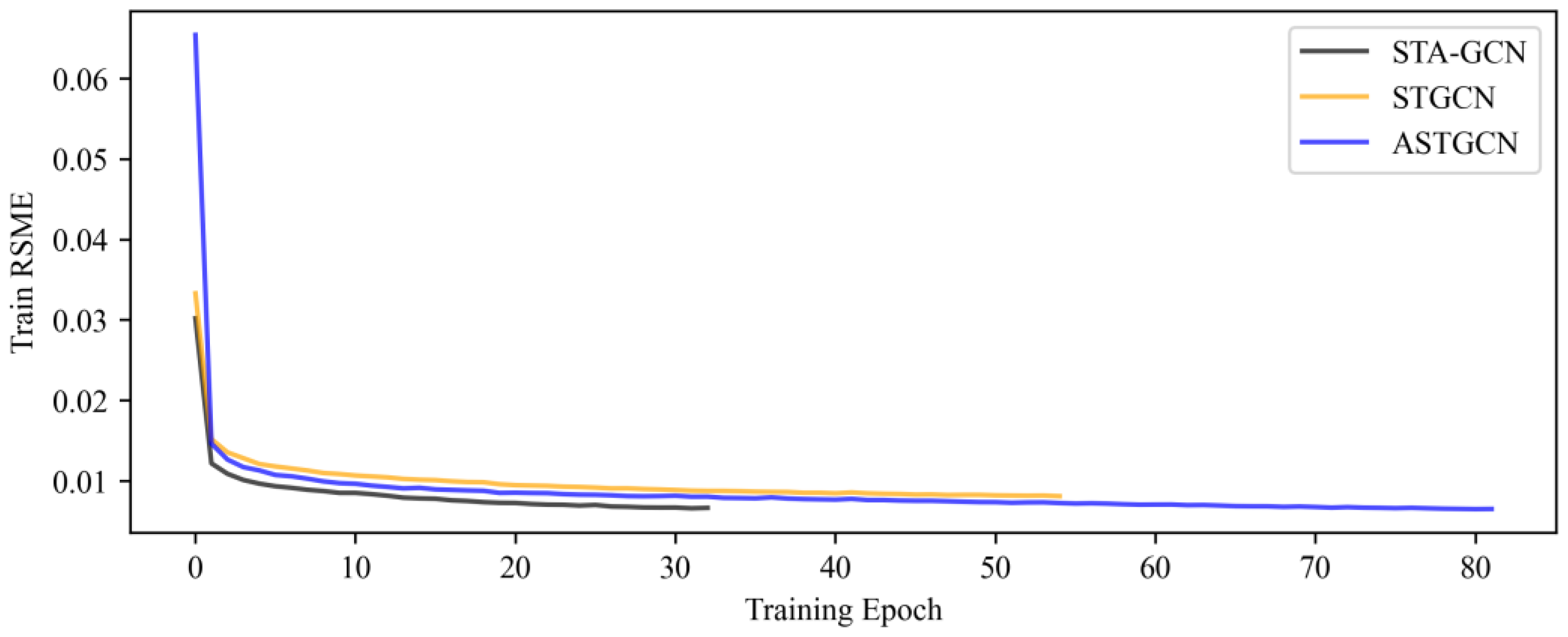
The training loss function of the model was considered to be converged when the validation set did not decrease further after ten epochs of training. Specifically, the number of training epochs and the final RMSE metric of the three types of model were compared when they reached convergence, as shown in Figure 6. It was found that the STA-GCN model had a faster convergence rate and lower prediction error.
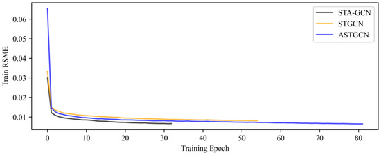
Figure 6.
Comparison of the number of training epochs and RMSE when three models converged.
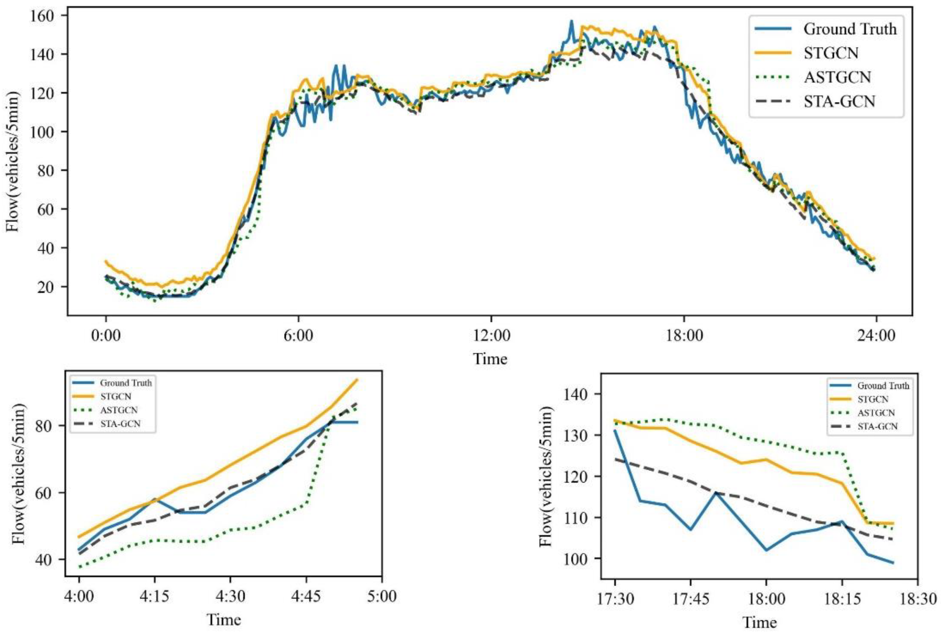
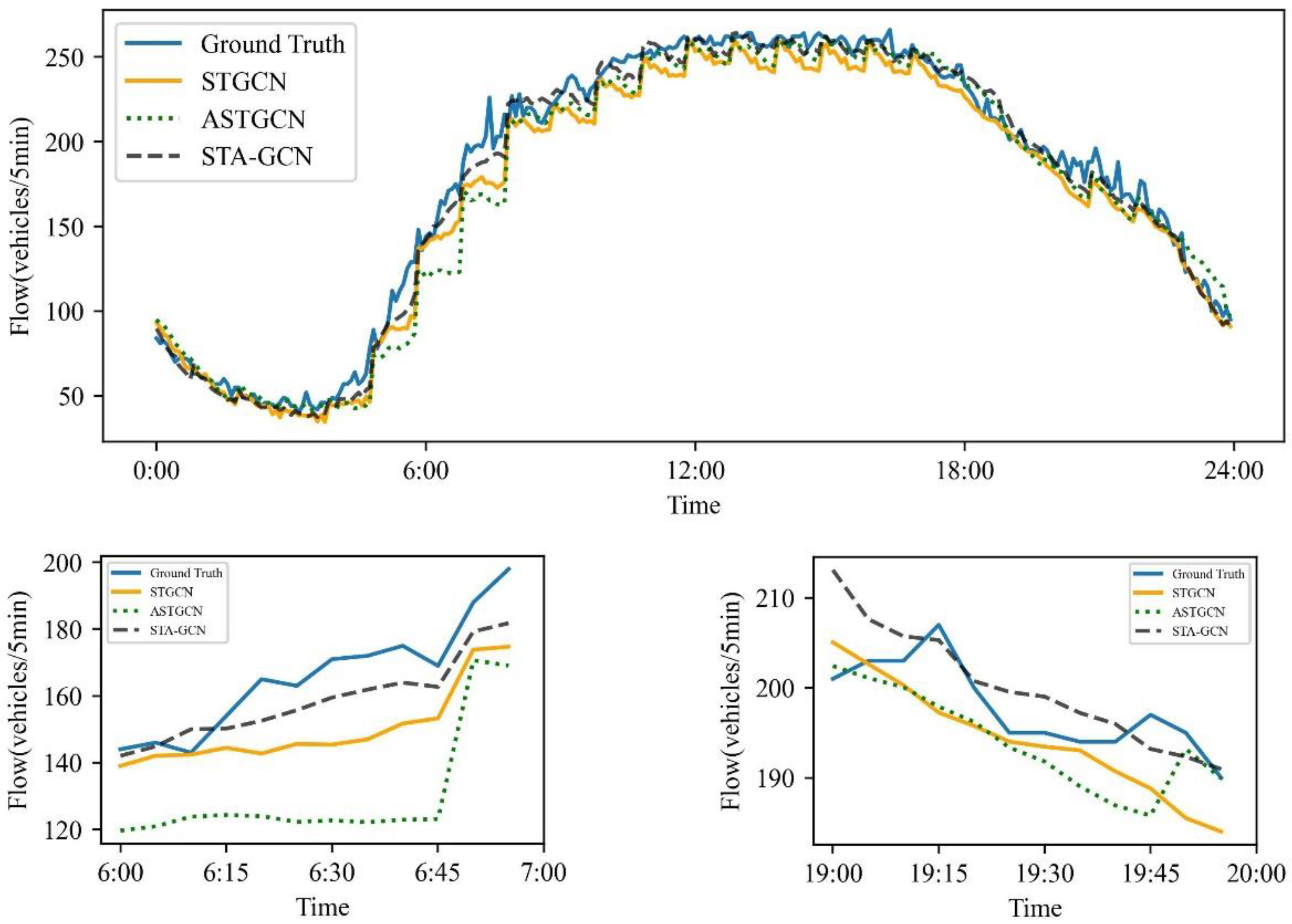
To further demonstrate that the predictive performance of STA-GCN is superior to that of STGCN and ASTGCN, we randomly selected one traffic node’s weekday and holiday prediction results from the PeMSD08 dataset for visualization. The visualization results for the weekdays are shown in Figure 7. During the time periods when the road-traffic volume suddenly increases (4:00–5:00) or decreases (17:30–18:30), STA-GCN can fit the trends in traffic-volume changes better than STGCN and ASTGCN. Similarly, the holiday prediction results are shown in Figure 8. During the time periods when the road-traffic volume suddenly increases (6:00–7:00) or decreases (19:00–20:00), STA-GCN can fit the trends in traffic-volume changes better than STGCN and ASTGCN.
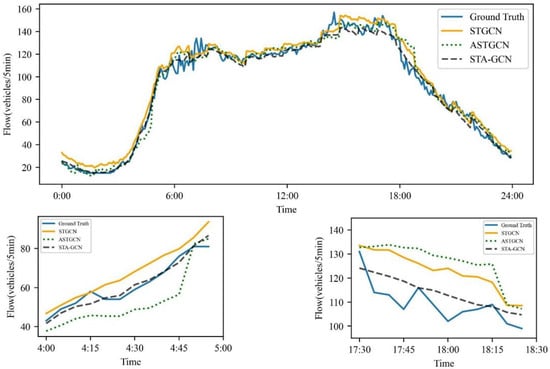
Figure 7.
Comparison of traffic-flow predictions on weekdays.
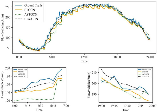
Figure 8.
Comparison of traffic-flow predictions on holidays.
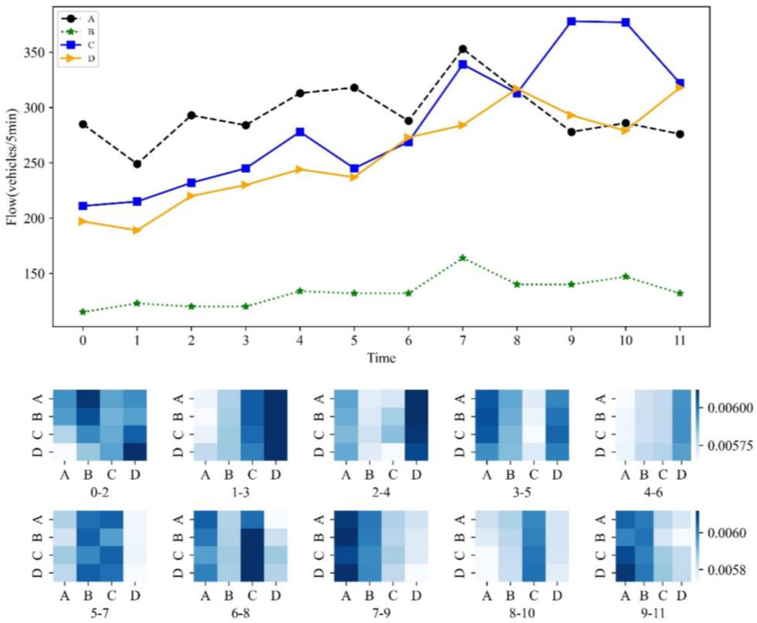
To better study the roles of the spatial self-attention mechanisms in the models, in Figure 9, the top image displays the traffic-flow changes of four randomly selected traffic nodes (A, B, C, and D) over the course of one hour. The bottom 10 images show the self-attention-score matrices of the four traffic nodes over 10 time intervals. In the 0–2 time interval, A has a higher attention score on B because the traffic-flow trends of the two nodes show a negative correlation during this time. In the 2–4 time interval, the attention scores of A, B, and C on D are the highest because the traffic flows of B and C are similar to that of D, and the traffic-flow trends are also similar. Moreover, A has a similar trend to D, and their traffic-flow increases are almost the same, at 20 and 24 respectively. Therefore, our model not only performs well in prediction but also has good interpretability.

Figure 9.
Visualization results of the spatial attention mechanism.
5. Conclusions
Traffic-flow prediction is an essential part of ITS research on improving traffic efficiency and safety. Both traffic managers and travelers can benefit from timely and accurate traffic-flow prediction. However, current spatial–temporal traffic-flow-prediction models rarely consider the periodicity and heterogeneity of traffic-flow changes from the network perspective.
To address this issue, in this paper, we proposed the spatial–temporal self-attention graph convolution network (STA-GCN) model, considering both periodic characteristics and the dynamic spatial–temporal dependence of network traffic flow. Specifically, Fourier decomposition was used to decompose the time series into periodic variables and one-hot encoding was used to distinguish the heterogeneity. Therefore, the proposed model incorporated spatial–temporal self-attention mechanisms into graph convolutional networks and time-gated convolutional networks to capture dynamic changes in traffic-flow characteristics.
Through a performance comparison with previous prediction models, the proposed model demonstrated a better performance on selected traffic-flow datasets, which indicates the effectiveness of STA-GCN in traffic-flow-prediction tasks. Furthermore, the visual analysis of the spatial-attention-prediction process was conducted to illustrate the interpretability of our model. Moreover, the proposed model is applicable to the prediction of other traffic parameters, including traffic speed and time occupancy, as well as passenger-flow predictions for subways and bus networks.
Although the STA-GCN model captures temporal–spatial traffic-flow patterns through the self-attention mechanism, the structure of the traffic-node network is fixed and unchanging. In future research, a promising method to improve the graph convolutional network would be to incorporate graph-theory-related approaches to enable the network to acquire dynamic characteristics. Furthermore, advanced neural network modules and more real-world datasets should be considered for integration into the prediction model.
Author Contributions
In this paper, Z.C. conducted the project administration, methodology, software, and original writing; C.L. conducted the data curation and validation; and J.J. developed the methodology for the factor analysis and performed the formal analysis, and review. All authors have read and agreed to the published version of the manuscript.
Funding
This research was funded by National Natural Science Funding (CN), grant number 41901396, and Youth Innovations Science and technology support project in Colleges of Shandong Province, grant 2021KJ058. The APC was funded by National Natural Science Funding (CN).
Institutional Review Board Statement
Not applicable.
Informed Consent Statement
Not applicable.
Data Availability Statement
The traffic-flow datasets PeMSD04 and PeMSD08 are open to the public and collected from the California Department of Transportation’s Performance Measurement System.
Acknowledgments
The authors would like to thank the support from the National Natural Science Foundation of China and the data support from Xuehui Chen and Shandong Hi-speed Company Limited.
Conflicts of Interest
The authors declare no conflict of interest.
References
- Zhang, J.; Wang, F.-Y.; Wang, K.; Lin, W.-H.; Xu, X.; Chen, C. Data-Driven Intelligent Transportation Systems: A Survey. IEEE Trans. Intell. Transp. Syst. 2011, 12, 1624–1639. [Google Scholar] [CrossRef]
- Lana, I.; Ser, J.D.; Velez, M.; Vlahogianni, E.I. Road Traffic Forecasting: Recent Advances and New Challenges. IEEE Intell. Transp. Syst. Mag. 2018, 10, 93–109. [Google Scholar] [CrossRef]
- Williams, B.; Hoel, L. Modeling and Forecasting Vehicular Traffic Flow as a Seasonal Arima Process: Theoretical Basis and Empirical Results. J. Transp. Eng. 2003, 129, 664–672. [Google Scholar] [CrossRef]
- Kumar, S.V.; Vanajakshi, L. Short-Term Traffic Flow Prediction Using Seasonal Arima Model with Limited Input Data. Eur. Transp. Res. Rev. 2015, 7, 21. [Google Scholar] [CrossRef]
- Cai, L.; Yu, Y.; Zhang, S.; Song, Y.; Xiong, Z.; Zhou, T. A Sample-Rebalanced Outlier-Rejected K -Nearest Neighbor Regression Model for Short-Term Traffic Flow Forecasting. IEEE Access 2020, 8, 22686–22696. [Google Scholar] [CrossRef]
- Jeong, Y.S.; Byon, Y.J.; Castro-Neto, M.M.; Easa, S.M. Supervised Weighting-Online Learning Algorithm for Short-Term Traffic Flow Prediction. IEEE Trans. Intell. Transp. Syst. 2013, 14, 1700–1707. [Google Scholar] [CrossRef]
- Dong, X.; Lei, T.; Jin, S.; Hou, Z. Short-Term Traffic Flow Prediction Based on Xgboost. In Proceedings of the IEEE 7th Data Driven Control and Learning Systems Conference (DDCLS), Beijing, China, 25–27 May 2018; pp. 854–859. [Google Scholar]
- Wang, S.; Zhao, J.; Shao, C.; Dong, C.; Yin, C. Truck Traffic Flow Prediction Based on Lstm and Gru Methods with Sampled Gps Data. IEEE Access 2020, 8, 208158–208169. [Google Scholar] [CrossRef]
- Lv, Y.; Duan, Y.; Kang, W.; Li, Z.; Wang, F.-Y. Traffic Flow Prediction with Big Data: A Deep Learning Approach. IEEE Trans. Intell. Transp. Syst. 2015, 16, 865–873. [Google Scholar] [CrossRef]
- Duan, Z.; Yang, Y.; Zhang, K.; Ni, Y.; Bajgain, S. Improved Deep Hybrid Networks for Urban Traffic Flow Prediction Using Trajectory Data. IEEE Access 2018, 6, 31820–31827. [Google Scholar] [CrossRef]
- Huang, X.H.; Tang, J.; Yang, X.F.; Xiong, L.Y. A Time-Dependent Attention Convolutional Lstm Method for Traffic Flow Prediction. Appl. Intell. 2022, 52, 17371–17386. [Google Scholar] [CrossRef]
- Scarselli, F.; Gori, M.; Tsoi, A.C.; Hagenbuchner, M.; Monfardini, G. The Graph Neural Network Model. IEEE Trans. Neural Netw. 2009, 20, 61–80. [Google Scholar] [CrossRef] [PubMed]
- Cui, Z.; Henrickson, K.; Ke, R.; Wang, Y. Traffic Graph Convolutional Recurrent Neural Network: A Deep Learning Framework for Network-Scale Traffic Learning and Forecasting. IEEE Trans. Intell. Transp. Syst. 2020, 21, 4883–4894. [Google Scholar] [CrossRef]
- Yu, B.; Yin, H.T.; Zhu, Z.X. Spatial-Temporal Graph Convolutional Networks: A Deep Learning Framework for Traffic Forecasting. In Proceedings of the 27th International Joint Conference on Artificial Intelligence, Stockholm, Sweden, 13–19 July 2018; pp. 3634–3640. [Google Scholar]
- Guo, S.; Lin, Y.; Feng, N.; Song, C.; Wan, H. Attention based spatial-temporal graph convolutional networks for traffic flow forecasting. In Proceedings of the AAAI Conference on Artificial Intelligence, Honolulu, HI, USA, 27 January–1 February 2019; Volume 33, pp. 922–929. [Google Scholar]
- Zhuang, W.; Cao, Y. Short-Term Traffic Flow Prediction Based on a K-Nearest Neighbor and Bidirectional Long Short-Term Memory Model. Appl. Sci. 2023, 13, 2681. [Google Scholar] [CrossRef]
- Huang, R.; Chen, Z.; Zhai, G.; He, J.; Chu, X. Spatial-temporal correlation graph convolutional networks for traffic forecasting. In IET Intelligent Transport Systems; John Wiley & Sons Ltd.: London, UK, 2023; pp. 1–15. [Google Scholar]
- Ma, Q.; Sun, W.; Gao, J.; Ma, P.; Shi, M. Spatio-temporal adaptive graph convolutional networks for traffic flow forecasting. In IET Intelligent Transport Systems; John Wiley & Sons Ltd.: London, UK, 2022; pp. 1–13. [Google Scholar]
- Cheng, Y.; Cheng, X.; Tan, M. Traffic Flow Prediction Based on Combination Model of ARIMA and Wavelet Neural Network. Comput. Technol. Dev. 2017, 27, 169–172. [Google Scholar]
- Tang, J.; Liang, J.; Liu, F.; Hao, J.; Wang, Y. Multi-community passenger demand prediction at region level based on spatio-temporal graph convolutional network. Transport. Res. Part C Emerg. Technol. 2021, 124, 102951. [Google Scholar] [CrossRef]
- Gilmer, J.; Schoenholz, S.S.; Riley, P.F.; Vinyals, O.; Dahl, G.E. Neural Message Passing for Quantum Chemistry. In Proceedings of the International Conference on Machine Learning, Sydney, Australia, 6–11 August 2017; Volume 70, pp. 1263–1272. [Google Scholar]
- Fang, S.; Zhang, Q.; Meng, G.; Xiang, S.; Pan, C. GSTNet: Global Spatial-Temporal Network for Traffic Flow Prediction. In Proceedings of the IJCAI, Macao, China, 10–16 August 2019; pp. 2286–2293. [Google Scholar]
- Li, Y.; Yu, R.; Shahabi, C.; Liu, Y. Diffusion Convolutional Recurrent Neural Network: Data-Driven Traffic Forecasting. In Proceedings of the International Conference on Learning Representations, Vancouver, BC, Canada, 30 April–3 May 2018; pp. 1–16. [Google Scholar]
- Song, C.; Lin, Y.; Guo, S.; Wan, H. Spatial-Temporal Synchronous Graph Convolutional Networks: A New Framework for Spatial-Temporal Network Data Forecasting. In Proceedings of the AAAI Conference on Artificial Intelligence, New York, NY, USA, 7–12 February 2020; Volume 34, pp. 914–921. [Google Scholar]
- Wu, Z.; Pan, S.; Long, G.; Jiang, J.; Zhang, C. Graph wavenet for deep spatial-temporal graph modeling. In Proceedings of the 28th International Joint Conference on Artificial Intelligence, Macao, China, 10–16 August 2019; pp. 1907–1913. [Google Scholar]
- Bruna, J.; Zaremba, W.; Szlam, A.; Lecun, Y. Spectral networks and locally connected networks on graphs. In Proceedings of the International Conference on Learning Representations (ICLR2014), Banff, AB, Canada, 14–16 April 2014; pp. 1–14. [Google Scholar]
- Defferrard, M.; Bresson, X.; Vandergheynst, P. Convolutional neural networks on graphs with fast localized spectral filtering. In Proceedings of the 30th International Conference on Neural Information Processing Systems, Barcelona, Spain, 5–10 December 2016; pp. 3844–3852. [Google Scholar]
- Diao, Z.; Wang, X.; Zhang, D.; Liu, Y.; Xie, K.; He, S. Dynamic Spatial-Temporal Graph Convolutional Neural Networks for Traffic Forecasting. In Proceedings of the AAAI Conference on Artificial Intelligence, Honolulu, HI, USA, 27 January–1 February 2019; Volume 33, pp. 890–897. [Google Scholar]
- Vaswani, A.; Shazeer, N.; Parmar, N.; Uszkoreit, J.; Jones, L.; Gomez, A.N.; Kaiser, L.; Polosukhin, I. Attention Is All You Need. In Proceedings of the Computation and Language, Long Beach, CA, USA, 4–9 December 2017; p. 3058. [Google Scholar]
- Dong, Y.; Liu, Q.; Du, B.; Zhang, L. Weighted feature fusion of convolutional neural network and graph attention network for hyperspectral image classification. IEEE Trans. Image Process. 2022, 31, 1559–1572. [Google Scholar] [CrossRef]
- Cai, L.; Janowicz, K.; Mai, G.; Yan, B.; Zhu, R. Traffic Transformer: Capturing the Continuity and Periodicity of Time Series for Traffic Forecasting. Trans. GIS 2020, 24, 736–755. [Google Scholar] [CrossRef]
- Xie, Y.; Niu, J.; Zhang, Y.; Ren, F. Multisize patched spatial-temporal transformer network for short-and long-term crowd flow prediction. IEEE Trans. Intell. Transp. Syst. 2022, 23, 21548–21568. [Google Scholar] [CrossRef]
- Yin, X.; Wu, G.; Wei, J.; Shen, Y.; Qi, H.; Yin, B. Deep Learning on Traffic Prediction: Methods, Analysis, and Future Directions. IEEE Trans. Intell. Transp. Syst. 2022, 23, 4927–4943. [Google Scholar] [CrossRef]
- Wen-Hsiung, C.; Smith, C.; Fralick, S. A Fast Computational Algorithm for the Discrete Cosine Transform. IEEE Trans. Commun. 1977, 25, 1004–1009. [Google Scholar] [CrossRef]
- Wen, C.; Zhu, L. A Sequence-to-Sequence Framework Based on Transformer with Masked Language Model for Optical Music Recognition. IEEE Access 2022, 10, 118243–118252. [Google Scholar] [CrossRef]
Disclaimer/Publisher’s Note: The statements, opinions and data contained in all publications are solely those of the individual author(s) and contributor(s) and not of MDPI and/or the editor(s). MDPI and/or the editor(s) disclaim responsibility for any injury to people or property resulting from any ideas, methods, instructions or products referred to in the content. |
© 2023 by the authors. Licensee MDPI, Basel, Switzerland. This article is an open access article distributed under the terms and conditions of the Creative Commons Attribution (CC BY) license (https://creativecommons.org/licenses/by/4.0/).

