1. Introduction
The technique of positron emission particle tracking (PEPT) has led to a paradigm shift in the measurement of flow behaviour in multiphase systems with high concentration of solids. PEPT can be applied to opaque experimental systems, as it relies on the detection of penetrating radiation from a tracer particle. The time-series location data produced by PEPT can also be used to plot high-resolution, time-averaged, or Eulerian maps of flow behaviour (e.g., [
1,
2]); additionally, it provides detailed Lagrangian paths of the tracer particle (e.g., [
3,
4]). For the three-phase mixture of mineral froth flotation, PEPT has revealed the paths and time-averaged flow profiles of particles of different mineral species (e.g., [
5,
6,
7,
8,
9]) and water [
10] inside a flotation vessel. It has also been used to track the interactions between particles and bubbles [
11].
However, questions still remain about whether high-frequency components of flow paths can be tracked effectively with PEPT. Some applications have removed these components as noise to focus on macroscale behaviour (e.g., granular flows [
12]), while others suggest that the high-frequency component of the motion displays microscale behaviour (e.g., liquid flows [
3]). This discrepancy has potential impact for applications of PEPT: either useful information about particle behaviour is being disregarded unnecessarily or information is output that could be a misinterpretation of the underlying particle behaviour.
In order to investigate the high-frequency component of the tracer particle’s motion, a model of the positron emission tomography (PET) scanner at PEPT Cape Town was developed, which produces simulated trajectories of a tracer particle moving on paths with characteristics of eddies and high-frequency fluctuations in turbulent flow. After validation with experimental data, the location data from the simulations can be compared to the ground truth path input to the simulation to determine the ability of PEPT measurements to represent turbulent flow paths.
1.1. Background of PEPT Measurements
PEPT can track the motion of tracer particles that have been radiolabelled with a positron emitting radionuclide and that share physical properties with the solid species in the system that is to be tracked [
13]. Positrons from the tracer radionuclide annihilate with electrons in the surrounding medium within the experimental system and produce pairs of almost colinear gamma ray photons. Two gamma rays that are detected within a short time window are labeled as being coincident, and the path of the gamma ray pair forms a virtual line of response (LOR) between two detectors in the scanner. The LOR traces a path indicating the potential source of the annihilation event. In any finite density medium, each point on the line has equal probability of being the location of the annihilation event, given that the LOR is a true coincidence. With multiple LORs recorded in a short time interval, the tracer particle can be located in the region of closest intersection of the LORs using a location algorithm. Time-series data of the tracer location can be compiled by selecting a sample of LORs and then applying a location algorithm to derive the tracer “location” in three dimensions at discrete time points
.
Different scanners specialised for PEPT applications have been adapted from their original medical imaging purposes to measure particle behaviour in systems of flow. These include the ADAC Forte [
14], Modular [
15], MicroPEPT [
16], and SuperPEPT [
17] cameras at the University of Birmingham, UK, where the PEPT technique was first developed [
18], and the Siemens ECAT EXACT3D HR++ camera at PEPT Cape Town at the University of Cape Town, South Africa [
19] (see
Figure 1; referred to as “HR++” henceforth). Other facilities specialising in PEPT measurements are the University of Tennessee, Knoxville in the US [
20] and the University of Bergen in Norway [
21].
1.2. Uncertainty in a PEPT Measurement
Every PEPT measurement contains inherent uncertainty from sources that include the detector configuration of the scanner, the positron range, the acolinearity of the photon pair, the sampling process, the resolution of the PET scanner, and the choice of tracking algorithm. Recent examples of location uncertainty quantification for PEPT measurements suggest values for different PEPT systems on the order of magnitudes 0.1 mm and 1 mm [
19,
23,
24,
25,
26,
27].
To minimise the uncertainty that arises from the method of deriving tracer locations, the size of the sampling window of LORs must be chosen with respect to timescales characteristic of the flow fluctuations and tracer activity. Using too few LORs leads to a loss of accuracy in the tracer location. With too many LORs, the tracer particle will move significantly within the window and also lead to a large uncertainty in the location measurements. The number of locations per unit time, or location rate, is also determined by the number of LORs used per sample and non-constant gamma ray attenuation due to the varying density of the local media [
28].
Uncertainty in a PEPT measurement also arises from temporal limitations of the PET scanner, specifically from the listmode timestamp output of the PET scanner. For the HR++, when coincidence data are being recorded, the timestamp is given to the nearest 1 ms. Therefore, PEPT measurements of flotation at PEPT Cape Town are performed with a conservative maximum location rate of 1 kHz [
29], calculated as the reciprocal of the timestamp. Higher location rates have been calculated for other PEPT systems by assuming an even distribution of the times of events within each timestamp [
21], using a small field of view (FOV) camera and an overlapping sampling window [
30], and with the SuperPEPT system [
17].
1.3. Simulation Tools to Improve PEPT Measurements
The Monte Carlo software GATE (Geant4 Application for Tomographic Emission) [
31,
32,
33] has been applied to PEPT measurements to explore different aspects of a PEPT measurement and the corresponding uncertainty [
24,
34,
35]. GATE is built upon the Geant4 (GEometry ANd Tracking 4) toolkit developed at CERN [
36]. GATE simulations are improving the treatment of PEPT data, specifically for the quantification of uncertainty in a PEPT measurement [
26], dynamic optimization of tracking parameters where the flow behaviour of the system is predictable [
37], validation with other simulation techniques such as Discrete Element Method (DEM) models [
28], and comparison with the performance of different PEPT location algorithms relative to the scanners commonly used for PEPT [
24].
One of the main advantages of GATE simulations for PEPT is that the true path of the tracer particle is known, since this is created as an input to the simulation. This can be used to determine the optimum reconstruction of time-series location data for PEPT measurements as well as to test the limits of PEPT as a technique and to determine if the PET scanner is able to track paths characteristic of a specific application, e.g., turbulent fluctuations in the flow of multiphase fluids. PEPT experiments are generally expensive to perform and time-consuming, making the use of GATE simulations valuable to optimise the parameters that decrease uncertainty in the measurement arising from the experimental protocol and data treatment.
1.4. Overview and Aim of This Work
This paper presents the development of a computational model in GATE to generate virtual paths for tracer particles and produce simulated lines of response to perform PEPT measurements. A series of validation tests was conducted, where physical experiments were performed with a tracer particle moving along defined paths to produce experimental lines of response. After deriving location data from the LORs with the PEPT-ML algorithm [
38], the location data from equivalent simulations were compared to the experimentally derived values to test if the accuracy and precision measured from the GATE simulation are comparable to those of the experimental data.
Once the model was validated, two different types of tracer motion were simulated to investigate the tracking ability (in terms of accuracy and precision) of PEPT measurements performed on the HR++ PET scanner. The extended simulations were inspired by the target application of this work, improving the tracking of turbulent flows in mineral froth flotation with PEPT (following [
8,
9,
10]). There do not yet exist sufficiently complex models of the interaction of the three phases in flotation that can produce Lagrangian trajectories of flow carriers of the solid, liquid, and gas phases to use with the HR++ PET scanner simulation (in comparison to recent studies with GATE and DEM simulations of granular flow [
28]). Instead, features of flow paths expected to be found in multiphase flows were reproduced. The first motion was an oscillation in a single dimension to explore the ability of PEPT to track high rates of acceleration (following [
24]) and the second was a helical path with constant tangential speed to explore the ability of PEPT to track turbulent vortices or eddies on different length scales. The tracking results were interpreted relative to the smallest eddies found in the water phase of flotation pulps with high energy dissipation rates to determine whether the PEPT measurement with the HR++ can reproduce Lagrangian paths of flow structures on the order of 10
m (in laminar flows) and 100
m (in turbulent flows) [
39].
2. Methods: Simulations with GATE
2.1. Model of the HR++ PET Scanner
The HR++ PET scanner (shown previously in
Figure 1) is managed by the Department of Physics at the University of Cape Town and is currently located at the iThemba LABS complex in South Africa. The scanner consists of 48 rings of bismuth germanate (BGO) crystals [
40]. The BGO crystals have dimensions of 4.39 mm × 4.05 mm × 30 mm (with a centre-to-centre spacing of 4.85 mm × 4.51 mm) [
40]. The crystals are arranged in 8 × 8 grids called blocks that are grouped into segments called “buckets” and composed of 6 detector blocks and their electronics (ADCs, preamplifiers, and discriminators), which can be physically removed. The cylindrical field of view (FOV) has a diameter of 82.0 cm and an axial length of 23.4 cm, which is significantly larger than a typical ring PET scanner.
The geometry used in GATE, including the array of detector elements, can be seen in
Figure 2, which included the absence of two detector buckets that were removed during measurements for repair and maintenance.
2.2. GATE Digitiser Parameters
The data acquisition and post-processing settings within the GATE simulation package are called digitiser parameters and include the coincidence timing window, the coincidence multiples policy (i.e., if more than two single events are detected within the same coincidence window), the minimum sector difference or span acceptance, dead time, energy blurring, and energy resolution. The specific digitiser parameters used in the HR++ detector model are listed in
Table 1.
2.3. Tracer Fabrication
Two types of tracer particle were used for the experiments and simulations. The polymethyl methacrylate (PMMA) cylindrical source, termed a “button” source, is 11.5 mm in height and 10.0 mm in diameter, with the activity located within a small conic section at the centre of the cylinder. Different versions of the button source were produced for the simulation, and the specifics of each use of this type of simulated source is henceforth referred to with the shorthand notation ButtonTracer [
A (
Ci),
RN], where
A denotes the activity of the radionuclide of species
RN. The second tracer type, the “NRW-100” tracer, is a spherical particle of varying radii and is composed of the ion exchange resin Purolite NRW-100 [
43]. It is referred to by the shorthand notation PointTracer [
A (
Ci),
R (
m),
], where
A denotes the activity,
R denotes the radius of the tracer in
m, and
denotes the radionuclide.
2.4. Tracer Configuration in the FOV
The tracer position in the FOV was configured in two ways for validation purposes: in a stationary position and while undergoing circular motion. Two shorthand notations are used: Stationary [X (mm), Y (mm), Z (mm)], where X, Y and Z denote the 3D coordinates of the tracer, and Circular [A (mm), f (Hz), (mm), (mm)], where A and f are the amplitude the frequency of the motion. For and , the subscripts a and b indicate the plane of rotation, while C identifies the centre of rotation within the specified plane.
2.5. Definitions
This subsection defines several terms that are used throughout this work. Any references to outputs of the simulation, such as “simulated location data” and “simulated data”, refer to the location data that were derived from the lines of response produced by the GATE simulation of the HR++ scanner. The location data were not produced directly by the simulation; instead, PEPT-ML was used to derive the locations from the simulated lines of response. Equivalently, “experimental location data” or “experimental data” refer to the location data that were derived from the lines of response recorded by the HR++ scanner during physical experiments. The terms “tracked location” and its time series equivalent “tracked path” can refer to the location data derived from either the experimental or simulated lines of response. This is also used generally to define metrics, and if a specific application was required, this is given. The “true” path refers to the ground truth path, which is used as an input to the simulation. It does not relate to the use of “true” in “true fraction” or “true coincidence”, which refer to the pairing of gamma rays to define coincidences when recording listmode data with the PET scanner. The term “PEPT measurement” is reserved for general application: it can be used for both experimental and simulation applications and refers to the entire process of obtaining an output location or series of locations, from the recording of the coincidence data to the derivation of a location.
3. Methods: Deriving the Location of the Source
For this work, the procedure used to convert the raw LORs into a series of locations was the same for both the experimental and simulated data. The source locations were calculated using the PEPT-ML package developed at the University of Birmingham [
38].
PEPT-ML is a machine learning tracking algorithm that first calculates the distance between all combinations of pairs of LORs in a given sample size (
). If two LORs are spatially closer than a user-defined maximum distance (
), they form a “cutpoint”, which is defined as the midpoint on the shortest line that connects the two LORs. After grouping all the LORs, the resulting cutpoints are then found using the Hierarchical Density-Based Spatial Clustering of Applications with Noise (HDBSCAN) algorithm [
44].
The PEPT-ML algorithm uses a true fraction (
) parameter to determine the fraction of cutpoints that are considered to arise from truly coincident LORs and classifies the remaining cutpoints as outliers [
38]. The final location of the tracer in 3D is then derived from an average of the positions of the remaining cutpoints. Once these locations are found, HDBSCAN can be applied again with a second pass in order to smooth and reduce noise of the first pass.
This algorithm requires seven parameters to run with two passes. The 7 parameters are: sample size 1 (SS1), overlap 1 (OL1), maximum distance (MD), true fraction 1 (TF1), sample size 2 (SS2), overlap 2 (OL2), and true fraction 2 (TF2). Each use of this algorithm is described with the parameters in shorthand by the term Clustering [SS1, OL1, MD (mm), TF1, SS2, OL2, TF2].
PEPT-ML was chosen for this work, instead of the more commonly used Birmingham algorithm, for convenience in applying multiple passes of HDBSCAN, which provide additional smoothing to reduce noise in location data. For example, there was a significant percentage reduction of ≈94% in positional error when comparing the PEPT-ML algorithm to the Birmingham algorithm when tracking two tracers undergoing circular motion at 42 RPM [
38]. It has been demonstrated to have increased precision for certain tracking scenarios [
38]. Its source code is also shared open source via the python package installer pip for easy implementation.
For the validation tests, the Clustering parameters were kept constant between equivalent tests in the simulation and experiments in order to remove any variations in the results due to the HDBSCAN parameters. These fixed parameters were chosen in such a way as to output location data with a location rate of approximately 1.0 kHz and to allow for a statistically meaningful comparison between the experimental and simulation results (e.g., avoiding the analysis of samples with very small or very large numbers of LORs that may not produce a location after processing with PEPT-ML). In the extended simulations, a gridsearch was used to find the parameter combination that minimised the difference between the output “tracked” path and the input “true” path. Unless otherwise specified, a combination of sample size (
) and overlap (
) parameters were used that met this minimum difference condition and output location rate of approximately 1.0 kHz. A short report giving further details on the procedure to optimise PEPT-ML for deriving location data from one of the extended simulations is given in
Appendix A.
The PEPT-ML parameters used for deriving location data as shown in all the results of this work can be found in
Appendix C,
Table A3 and
Table A4. The output location rate
L was calculated using
, where
B was the number of locations and
was the tracking time. The uncertainty in the location rate
was calculated using a counting uncertainty
. The location rates for all the results of this work can be found in
Appendix C,
Table A3 and
Table A4. An overlap in the first pass of PEPT-ML was not implemented in any of the results. Future research could study the impact of this parameter on the uncertainty in the measurement of the time variable of a location.
4. Methods: Experiments for Validation
In clinical uses of PET and other PEPT simulations, GATE simulations of PET scanners are routinely validated according to a standard of the National Electrical Manufacturers Association (NEMA), NEMA NU 2-2012 [
45]. In the present work, it was not possible to use NEMA NU 2-2012, as the HR++ scanner does not record single event data. Instead, coincidence data have been used to show that the GATE simulation produces similar LOR data to equivalent physical experiments by comparing locations from PEPT measurements.
Three sets of experiments were performed to correspond to simulations consisting of either a stationary or a moving source. Measurements of the location of a stationary tracer with decreasing activity were used to assess whether the simulated geometry and the detector and digitiser settings produced comparable coincidence rates between experiment and simulation over the changing activity of the source. Measurements of the location of a stationary tracer in different positions around the scanner FOV were used to directly compare the uncertainty in the location between experiments and the GATE simulation. Measurements of circular motion were used with experimental data to validate the HR++ model’s ability to simulate the tracer undergoing motion on two paths of different radii and rotational frequency.
4.1. Experiment: Stationary Source with Decreasing Activity
This experiment was performed with a button tracer with activity of 20 Ci Ga located at the centre of the FOV. Due to the short half-life of Ga ( = 68 min), it was possible to perform measurements of the same location over a wide range of activities. There were a total of eight samples of LORs recorded over 7 h and 55 min, with each recording 120 s in duration and timed to occur between intervals when the tracer activity reduced by half, i.e., every 68 min. The source was formed by evaporating 10–15 L of the Ga solution in the centre of the button tracer before sealing the source. Gaussian fits were performed on the experimentally derived location data to find the average location to use as the ground truth in the corresponding simulations.
4.2. Experiment: Stationary Source in Different Positions
A button tracer with 60
Ci
Na was placed at multiple locations within the FOV of the HR++, as shown in
Figure 3. The experimental locations can be found in
Appendix C,
Table A1, and these locations were used as the ground truth location in each simulation. The stationary source was formed in a similar way as reported previously for the button source, with
Na as the radionuclide instead. The acquisition was performed by saving the listmode data every 120 s.
4.3. Experiment: Moving Source on a Circular Path
Two PEPT experiments were performed of a tracer particle following a circular path. The first experiment was a button tracer with 60
Ci
F activity undergoing circular motion. The amplitude and frequency were 71.19 mm and 1.06 Hz, respectively. The circular motion took place in the
plane, with the centre of the circular motion at
X = −1.30 mm and
Y = −0.54 mm, and the listmode data were acquired with a 5.0 s duration. The source was formed as before with
F as the radionuclide. The tracer was attached using adhesive to a wooden rotating disc with a radius of approximately 70 mm. The second experiment was performed with an NRW-100 tracer of radius 400
m with 591
Ci activity of
Ga. The NRW-100 tracer underwent circular motion with an amplitude and frequency of 27.64 mm and 19.74 Hz, respectively. The circular motion took place in the
plane, with the centre of the circular rotation at
X = 1.14 mm and
Z = 1.73 mm, with a 0.5 s duration of listmode acquisition. The tracer was attached using adhesive tape to a wooden disc with an approximate radius of 30 mm. It should be noted that the parameters describing the circular motion were calculated from the sinusoidal fits described by the circular motion [
46], to produce a series of locations derived from processing experimentally obtained LORs with PEPT-ML to achieve a location rate of approximately 1.0 kHz. These fit parameters for the circular motion were then used to define the ground truth in the corresponding simulations.
During processing, additional oscillations were observed in the experimentally derived location data that likely arose from additional vibrations in the equipment. These were added to the model, and there is a short description of the implementation in
Appendix B.
5. Results: Model Validation
Each of the three experiments described in
Section 3 was simulated using the HR++ GATE model.
5.1. Validation with Coincidence Count Rate Data
The coincidence rates from the experiments and simulations of a stationary tracer particle with decreasing activity can be seen in
Figure 4. There is strong agreement between the experiment and simulation coincidence rate data with activity. Linear fits were applied to the data, and the gradients obtained from the experimental and simulated coincidence data were 1295 ± 22 s
Ci
and 1279 ± 9 s
Ci
, respectively, which agree within one standard uncertainty. All fits and uncertainties were computed using LMFIT [
47]. The vertical offsets for the linear fits to the experimental and simulated coincidence data were 1170 ± 179 s
and 1151 ± 74 s
, which also agree within one standard uncertainty.
5.2. Validation with Location Data from a Stationary Tracer
The experiments with the tracer particle at different stationary positions within the FOV of the HR++ scanner, as shown in
Figure 3, were also simulated using the ButtonTracer [60
Ci,
Na] in the HR++ GATE model.
Figure 5 shows examples of the LOR distributions from experiments and simulations at Position O (see
Figure 3). There were two missing buckets during the experiments, and they were removed from the simulation. Both plots show the sites of the missing buckets as areas where no events were detected. Due to the stochastic nature of the nuclear interactions involved in PET, the simulation will never reproduce an identical combination of LORs as found in the experiments.
The experimental and simulated LOR data from a stationary tracer particle were processed using PEPT-ML to produce a series of tracer locations as shown in
Figure 6. Gaussian functions were fitted to the distributions of locations to find a mean location with a standard uncertainty value in order to compare the simulated and experimental values, the full results of which can be found in
Appendix C,
Table A1. In order to compare the deviations from the ground truth between the experiments and simulations, Equation (
1) was applied to the location data with time, where
is the difference in position as calculated between a location
i on the tracked path (
) and the ground truth path at the time value taken from the tracked path (
), and
N is the number of locations. The parameter
will be referred to as the average path uncertainty.
Figure 6 shows agreement between locations derived from the HR++ model and the experiments, as the fitted Gaussian distributions have similar profiles. This point is reinforced by a comparison of the mean and standard uncertainty values from the fits as given in
Table 2 where the intervals overlap, and thus the experiment and simulation results agree within experimental uncertainty. A similar analysis for the other FOV positions is given in
Appendix C,
Table A1.
5.3. Validation with Location Data from a Tracer Undergoing Circular Motion
For the circular motion experiments described in
Section 4, the location data derived from simulations and experiments were used to produce 1D profiles of the motion in the
X,
Y, and
Z dimensions, as shown in
Figure 7. The amplitude and frequency fit parameters can be seen in
Appendix C,
Table A2, which are generally in agreement to one standard uncertainty.
Location data from PEPT measurements of the NRW-100 PointTracer [591
Ci, 400
m,
Ga] moving on a different circular path are shown in
Figure 8, with a location rate of approximately 1.0 kHz. This motion has higher speeds than the other circular motion shown in
Figure 7. The amplitude and frequency fit parameters can be seen in
Appendix C,
Table A2. The Gaussian fits to the distributions of the true and tracked locations are generally not in agreement within one standard uncertainty.
An alternative method to compare the measurements of location data between the experiments and simulations is the path uncertainty (Equation (
1)).
Table 3 and
Table 4 show the values of the path uncertainty for the 2 different circular motions used in the validation tests. The path uncertainty is less sensitive to small variations in the centre of the circular motion and starting position on the path, which can lead to differences between the parameters of the sinusoidal fits to the experiment and simulated location data that are greater than one standard uncertainty. The paths for both the ButtonTracer and PointTracer undergoing circular motion at different speeds show similar values in the path uncertainty regardless of whether they were calculated from experimental or simulated location data.
6. Results: Simulations of Extended Scenarios
Having validated the HR++ GATE model under the above-described scenarios, the ability of the model to track a tracer particle in different situations that represent important features of a particle moving in a turbulent fluid are investigated.
6.1. Modes of Tracer Motion
Two additional types of motion were introduced to the GATE model: a non-sinusoidal oscillatory motion and a spiral motion. For the non-sinusoidal oscillatory motion, the motion is described by
where the parameters include frequency
f and the amplitude of the motion
Q [
48]. A plot showing the motion of Equation (
2) can be seen in
Figure 9.
The shorthand notation for the simulations of oscillatory motion is Oscillatory [
Q (mm),
f (Hz)]. The oscillatory motion was used previously to explore the ability of different location algorithms for PEPT to track the tracer at the turning points of a path [
49] and offers an alternative test to the circular path used in other works (e.g., [
18,
19,
29]). The oscillatory motion was chosen for this work to give insight into the ability to track tracer motion at the turning points of a path. The tracer particle has infinite acceleration at the turning points, a feature that occurs in high-frequency fluctuations as could be expected in turbulent multiphase flow paths.
The spiral motion was a constant linear velocity (CLV) spiral in the
plane, which has a constant tangential velocity independent of the radius of the spiral. The polar position (
,
r) has two coordinates as a function of time
t,
and
The parameters describing the spiral are
, the spiral separation or sampling pitch along the radial direction, and
V, the instantaneous velocity [
50].
Thus, the coordinates of the
position of the tracer on the spiral at a given time
t are
with a constant
Z value.
A shorthand notation for the simulation of the spiral motion is Spiral [ (mm), V (ms)]. This motion was chosen to test the ability of PEPT measurements with the HR++ scanner to track the structure of eddies of different length scales that appear in turbulent, multiphase fluids.
6.2. Tracking a Particle in Oscillatory Motion
Two simulations were run using a PointTracer [1100
Ci, 300
m,
Ga] with Oscillatory [100 mm,
Hz] in the
X direction. This particle was chosen to represent the type of particle used in published examples of PEPT measurements of multiphase flow and the type of tracer particle that is routinely fabricated for experiments at PEPT Cape Town with the HR++ scanner [
13].
Two cases of oscillatory motion for extreme values of velocity have been highlighted in
Figure 9, with
Figure 9a,c representing the low-speed (0.5 m s
) path and
Figure 9b,d showing the high-speed (25.0 m s
) path. For the low-speed path (
Figure 9a,c), the location data of the tracked path tend to be close in value to those of the true path, as illustrated by small values of the residuals. Near the turning points, the absolute values of the residuals tend to be larger but are mostly within an acceptable range of
m defined by the size of the tracer. This range is referred to as acceptable because it is expected that positrons from the tracer generally annihilate within or close to the material of the tracer particle when placed in dense media such as water and solid particle mixtures [
25].
Looking at the high-speed path (
Figure 9b,d), there is a significant difference as compared to the low-speed case in the tracking fidelity of the oscillatory motion. On the straight portions of the trajectory, the tracer particle experiences a constant velocity, and the residuals are low along this path. However, near the turning points, the residuals are considerably larger. During constant linear motion and within a given time window, an average of multiple tracer positions will tend to be a good measure of the true position of the tracer particle at the middle of the time window. In contrast, during linear acceleration, the averaging process will not cancel out those tracer positions that were taken before or after the middle of the time window. This will lead to large uncertainty in the tracer location whenever a tracer is undergoing acceleration during any given time window. Calculation of an average residual over several cycles of the oscillatory motion would tend to a small value, close to zero, but would misrepresent the overall distribution of residuals over each cycle, which are significantly larger near the turning points.
Therefore, the large deviation in
X arising at the turning points of the oscillatory motion in
Figure 9 is due to the non-symmetric distribution of the LORs in the samples around the turning points. This asymmetry is caused by the infinite acceleration about the turning points, which shifts the mean of the distribution of cutpoints used in each location to a point before/after the turning point.
Examples of the distributions of cutpoints used in samples both at and in between the turning points of the motion are given in
Figure 10 to illustrate this behaviour. The distribution of cutpoints in the sample near the turning point (see
Figure 10a) is narrower and tends to have more weight to the right (in this case) of the true value of the location. The tracked location occurs 3.89 mm away from the true location. A smaller deviation of the tracked location from the true location of 0.30 mm is visible in
Figure 10b for the location on the linear part of the motion, with cutpoints distributed symmetrically and around the true location.
6.3. Tracking a Tracer Particle on a Spiral Path
The parameters that describe the spiral simulation were Spiral [0.1 mm, 0.8 m s
] for a simulation time of
s with the tracer PointTracer [1000
Ci, 300
m,
Ga]. The location data with time can be seen in
Figure 11. The combination of a path with low speed and a tracer particle with high radiolabelled activity was used to ensure that as many locations as possible were present on the parts of the spiral path with smaller radii. The spiral gets larger in radius as time increases and allows for the determination of the smallest structure that can be tracked on a Lagrangian path with the HR++ scanner in terms of the minimally tracked radius.
In the first 0.2 s of
Figure 11d, the residuals are the largest, showing an inability to track the spiral path of the smallest radii considered, which correspond to the higher rates of acceleration experienced by the tracer.
To analyse the spiral tracking results in more depth, the uncertainty in the path
was calculated with Equation (
1), where the residual
is defined as the difference between samples of locations from the true and tracked paths.
Figure 12 shows the results as a function of radius and magnitude of acceleration. In
Figure 12a, the uncertainty in the path tends to decrease with increasing radius for a tracer moving along the spiral path. For radii larger than 2.0 mm, the uncertainty tends to an asymptotic value of around 0.25 mm, which is similar in magnitude to the radius of the tracer particle. For radii smaller than 2.0 mm, the uncertainty is considerably larger than the size of the tracer, suggesting that, within this spiral, the PEPT measurement is unable to reliably track structures smaller than 2.0 mm with a Lagrangian path. The uncertainty in the path as a function of acceleration is shown in
Figure 12b, where the acceleration tends to increase with a decreasing radius. For locations on the spiral path with acceleration values less than approximately 400 m s
, the uncertainty in the path was smaller than the radius of the tracer particle.
7. Discussion
Considering the results of the validation tests performed to compare location data from experimental LORs with the output of the GATE simulation of the HR++, it was shown that the HR++ model is an effective model for PEPT measurements of stationary and moving tracer particles. Specifically, the experiment and simulation location data show agreement within one standard uncertainty for the measurements of the location of a stationary source in different positions around the FOV of the PET scanner, agreement within one standard uncertainty of the parameters of sinusoidal fits to the path of a tracer particle moving on a circular path at low frequency, and agreement in the path uncertainty of a tracer particle moving on a circular path at high frequency. Similarity between PEPT measurements performed in experiments and simulations with different types of tracer particles (button and point) and three different radionuclides (
F,
Na,
Ga) were demonstrated to broaden the application of the model. This validation is not as rigorous as performing the tests advised by the standard protocol NEMA NU 2-2012 [
45], which compare measurements between experiments and corresponding GATE simulations in terms of the spatial resolution, scatter fraction, sensitivity, accuracy, and image quality. The standard is used by the medical imaging community and, more recently, by developers of PEPT as a technique at the University of Birmingham [
37]. In the absence of the appropriate data from experiments with the HR++ scanner, in particular single-event data, the work presented here used coincidence data to demonstrate the validity of the HR++ GATE model to reproduce PEPT measurements of tracer particles both stationary and moving, where the motion is predictable. Future research will explore the validity of the simulation for scenarios far removed from those presented here, while the current model will be used to develop improvements to data processing techniques and interpretation of PEPT measurements of multiphase flows.
The GATE simulations were also used to explore PEPT measurements of tracer particles moving on paths characteristic of flow paths where turbulence is present. When tracking a particle of routine fabrication at PEPT Cape Town (radius 300 m and activity 1000 Ci) on an oscillating path, it was illustrated that PEPT can track high-speed, linear sections of the path; however, sampling artefacts introduce large uncertainty into the PEPT location measurement on the turning points of the path. Specifically, when using a sample of LORs to derive a tracer location, if the tracer does not accelerate within the temporal window, the average location will tend to be on the true path without significant deviation from the true path. This deviation was measured to be 0.30 mm, a size similar to that of the tracer particle. On the other hand, if the tracer experiences acceleration within the sampling temporal window, the average location may not tend to be on the true path, with considerable deviation of over 3 mm. This is likely a regular occurrence when tracking the turning points of high-speed paths. These results illustrate the potential of this sampling artefact to reduce the amplitude of high-speed fluctuations in the path of turbulent, multiphase flows in regions where there is high particle acceleration. Using the order of magnitude of the deviation of the tracked path from the true path at the turning points, PEPT measurements with the HR++ would be unable to accurately track fluctuations smaller than a millimetre scale.
Simulations were also performed of a tracer particle moving on a spiral path and showed that measurements with the HR++ are able to track spiral structures with radii larger than or equal to 2.0 mm, to an uncertainty smaller than the size of the tracer particle. Tracking the path to smaller radii led to an increase in the location uncertainty in terms of an increasing deviation from the true path. The size of the tracer particle is suggested as an acceptable uncertainty based on several assumptions of the radiolabelling of the tracer particle, as the role of positron range has not yet been determined in location calculations with the routine tracer particles. It is expected that the radionuclide is contained in a surface layer of the NRW100 resin material; therefore, positrons from the tracer particle will tend to annihilate within the resin. In practice, this is likely to underestimate the average range of the positron, and it remains an area of future work for GATE simulations to relate the positron range in different media to the accuracy and precision of location measurements.
The threshold for fluctuations presented here, which is on the order of magnitude of 1 mm based on results of 2–3 mm from the oscillating and spiral simulations, is considerably larger than the size of the tracer particle and the size of the smallest eddies found in the water phase of flotation pulps, 10 and 100
m for laminar and turbulent flow, respectively [
39]. However, it is a matter of debate whether particles of the same size as the tracer particle can experience the interior of these microscale eddy structures, and tests with smaller tracer particles were not performed. In combination with the threshold for location uncertainty of the size of the tracer particle, the results presented here suggest that PEPT measurements with the HR++ have greater applicability to systems using larger tracer particles (for a larger acceptable location uncertainty) and with larger fluctuations and characteristic length scales of turbulence.
Further work is required to extend the scope of the simulations and explore the role of the varying density of the local media, the tracer activity, and the size of the tracer particle; however, the results of the simulations included here suggest that PEPT measurements performed with PET scanners with lower spatial resolution and/or lower tracer activity would tend to have poorer ability to track turbulent fluctuations than demonstrated in this work.
The uncertainty in the measured locations could be reduced by using a different radionuclide for the tracer fabrication, where
F generally has a shorter positron range in dense media [
51], and by employing a PET scanner with higher instrinsic spatial resolution, such as the microPET system at the University of Tennesse, Knoxville [
20] or SuperPEPT at the University of Birmingham [
17]. These improvements may make feasible PEPT measurements with smaller tracer particles which, based on current methods for tracer fabrication, are associated with lower radiolabelled activity and would tend to increase the uncertainty values given here.
The location rate of the presented PEPT measurements is also significant, where the 1.0 kHz threshold ensures a large sample of LORs are used in the calculation of each location. Where the tracer particle does not move within the sample temporal window, this leads to the calculation of a location with high precision. However, where the particle moves within the window, such as on the spiral path with radii smaller than 2.0 mm, an increase in location rate could be achieved with an overlapping sample size or dynamic sample size. A higher location rate has the potential to improve the tracking result and enable the tracking of the path to smaller radii. For similar impact, the data acquisition hardware of the HR++ scanner could be improved, ideally to record the time of each LOR to a higher precision than the 1 ms timestamp.
8. Conclusions
A computational model of the Siemens ECAT “EXACT3D” HR++ PET scanner was constructed in GATE to explore the ability of PEPT measurements at PEPT Cape Town to track flow behaviour in multiphase applications such as mineral froth flotation. The model was validated for PEPT research by measuring the coincidence rate over a range of activity radiolabelled on the tracer particle and by comparing tracer locations calculated from the GATE simulation to values acquired from experiments with stationary and two moving sources at varying speeds.
The model was then used to explore two extended scenarios that were used to investigate the tracking of turbulent fluctuations. Using simulations of a path with non-sinuoidal oscillation in 1D, the location data from PEPT measurements at a typical location rate of 1 kHz were able to track high-speed, linear motion but unable to track the turning points in the motion. Following a tracer on a simulated spiral path, the uncertainty in the location increased as the size of the spiral decreased. Above a radius of 2.0 mm, the PEPT measurement tracked the path of the spiral to an uncertainty less than the size of the tracer particle, ≈300 m, and below a 2.0 mm radius of the spiral. The location uncertainty increased beyond this threshold due to the high acceleration along the helical path.
In conclusion, for the benefit of the host facility for this research, PEPT Cape Town at the University of Cape Town, the validated GATE model presented can be used to explore more complicated flow situations, providing realistic data to aid in experimental design, and to better understand the limitations of the HR++ detector. Future applications for the HR++ model that are currently underway include: optimising measurement parameters at iThemba LABS by being able to initially run an experiment virtually; advancing tracer development by looking at an extensive range of materials, shapes, and sizes to determine the best combination for a given situation, even possibly providing custom tracers; and extending the work to include investigations into dynamic sampling with field-of-view attenuation to improve the tracking of turbulent, multiphase flows.
Author Contributions
Conceptualization, R.P., K.C., S.W.P., J.S. and P.R.B.-P.; methodology, R.P., K.C., J.S. and S.W.P.; software, R.P., S.W.P. and K.C.; validation, K.C., S.W.P., J.S. and P.R.B.-P.; formal analysis, R.P.; investigation, R.P., K.C., M.R.v.H., Y.-Y.L. and J.Z.; resources, K.C., S.W.P., A.B., M.R.v.H. and P.R.B.-P.; data curation, A.B., K.C., S.W.P., P.R.B.-P. and M.R.v.H.; writing—original draft preparation, R.P., K.C. and S.W.P.; writing—review and editing, R.P., K.C., S.W.P., J.S., P.R.B.-P., A.B., Y.-Y.L., J.Z. and M.R.v.H.; visualization, R.P.; supervision, K.C., S.W.P. and J.S.; project administration, S.W.P. and K.C.; funding acquisition, K.C., R.P., S.W.P. and P.R.B.-P. All authors have read and agreed to the published version of the manuscript.
Funding
This research was funded by the University Research Council at the University of Cape Town (1551680) and the National Research Foundation (NRF) through their DSI-NRF First Time Doctoral Scholarships (PMDS22060920524).
Data Availability Statement
The data and simulations presented in this study are available on request from the corresponding author.
Conflicts of Interest
The authors declare no conflict of interest.
Abbreviations
The following abbreviations are used in this manuscript:
| ADC | Analogue-to-Digital Converter |
| BGO | Bismuth Germanate |
| CLV | Constant Linear Velocity |
| DEM | Discrete Element Methods |
| ELR | Location Rate of Experimentally Derived Data |
| FOV | Field of View |
| GATE | Geant4 Application for Tomographic Emission |
| Geant4 | GEometry ANd Tracking 4 |
| HDBSCAN | Hierarchical Density-Based Spatial Clustering of Applications with Noise |
| LOR | Line of Response |
| MD | Maximum Distance |
| NEMA | National 128 Electrical Manufacturers Association |
| OL1 | Overlap 1 |
| OL2 | Overlap 2 |
| PEPT | Positron Emission Particle Tracking |
| PEPT-ML | Positron Emission Particle Tracking Machine Learning |
| PET | Positron Emission Tomography |
| PIV | Particle Image Velocimetry |
| PMMA | Polymethyl Methacrylate |
| RN | Radionuclide |
| SLR | Location Rate of Simulation-Derived Data |
| SS1 | Sample Size 1 |
| SS2 | Sample Size 2 |
| TF1 | True Fraction 1 |
| TF2 | True Fraction 2 |
Appendix A. Optimisation of PEPT-ML for Extended Scenarios
The location data from the simulated LORs for
Section 6.2 and later subsections in
Section 6 were derived with an optimisation procedure with PEPT-ML that sought to find the parameter combination over two passes of the algorithm that led to the minimum location uncertainty for a target location rate, where the path uncertainty is a measure of the difference between the tracked and true paths as given in Equation (
1). Using results from the simulation of non-sinusoidal oscillation described in
Section 6, this is a short report on the methods used to optimise PEPT-ML with data that have a ground truth.
It should be noted that, in theory, there will be different optimal combinations of the parameters for PEPT-ML when considering the turning point of the path and the part in constant motion for the simulated data in
Section 6.2. However, in practice, it is difficult to know when processing experimental data whether the tracer is moving on a constant velocity path or an accelerating path. Therefore, a set of parameters was used to produce location data with a
global minimum of path uncertainty, which was derived with data from both characteristic sections of the path (linear and turning point). For the first pass, a gridsearch was used to find the optimal sample size
as shown in
Figure A1a, noting the overlap
was set to 0, as mentioned previously.
The
optimisation can be seen in
Figure A1b, which ended once a minimum location uncertainty had been found. There was little reduction in the uncertainty for different values of
, which is possibly related to the measurements being performed in the centre of the field of view of the scanner, a region with the highest geometric efficiency and with no other attenuating materials present. A value for the overlap of the second pass
was then found, as shown in
Figure A1c, where the second pass of the PEPT-ML algorithm reduces the uncertainty in the tracked path by smoothing and removing outliers that might be present in the first pass. This leads to a further reduction in the location uncertainty, which can be seen from comparing
Figure A1a,c. The optimisation process was stopped once a parameter combination had been found that corresponded to a target location rate of approximately 1.0 kHz.
Figure A1.
The optimisation procedure for the PEPT-ML algorithm to find the optimal combination of tracking parameters for the simulations of Oscillatory [100 mm, 62.5 Hz] motion path for a PointTracer [1100 Ci, 300 m, Ga]. For the first pass, (a) shows the path uncertainty in the X dimension of the oscillatory motion and location rate L of the tracked path for different sample sizes with maximum distance and true fraction set to 1.8 mm and 0.6, respectively. (b) for different values of the true fraction with and set to 2.0 mm and 140, respectively. For the second pass, (c) shows and location rate L of the tracked path for different sample sizes with set to 0.6. (d) as a function of true fraction with set to 5, and the overlap set to 4. The shaded regions show a threshold of uncertainty of ≤0.3 mm, which is the radius of the tracer.
In
Figure A1d, the uncertainty stays constant and then suddenly decreases to a lower value, which is caused by the low true fraction removing a significant number of locations at a low
due to the low
. Once the
reached 0.5, enough points remained that HDBSCAN was able to cluster these locations from the first pass of tracking.
The maximum distance
optimisation can be seen in
Figure A2, where the optimal
value was found to be 2.0 mm due to a diminishing reduction in uncertainty for higher values. In the main implementation of PEPT-ML [
38], a value of
= 0.1 mm to 0.2 mm is recommended; however, a value of 2.0 mm leads to a lower uncertainty for the measurements presented here. This is likely due to the use of a different camera configuration with the testing of PEPT-ML.
In summary, the optimal parameters for Oscillatory [100 mm, 62.5 Hz] motion were found to be Clustering [140, 0, 2.0 mm, 0.55, 5, 4, 0.50]. The value of
= 140 was selected as giving a location rate of approximately 1.0 kHz. This appears to be optimal for this experiment because a higher location rate leads to an uncertainty larger than the tracer size, while a lower location rate produces a lower uncertainty but fewer locations to maintain tracking accuracy (see
Figure A1). The value of
is always 1 less than
, to maintain a constant location rate while smoothing the data relative to nearby locations.
Figure A2.
Uncertainty
as a function of maximum distance
in mm. The
and
values were set to 140 and 0.6, respectively. The other parameters for the PEPT-ML optimisation procedure are given in
Figure A1.
Figure A2.
Uncertainty
as a function of maximum distance
in mm. The
and
values were set to 140 and 0.6, respectively. The other parameters for the PEPT-ML optimisation procedure are given in
Figure A1.
Appendix B. Fixed Axes Vibrations in the Circular Motion
In two of the validation tests following a tracer particle on circular paths, as described in
Section 4, the motion was constrained to 2 dimensions. The third dimension of the locations in both cases should have been a constant with time; however, in experiments, it was observed to show additional oscillations that tended to increase the uncertainty in the sinusoidal fits to the simulated location data. These vibrations in the fixed axes of rotation of the location data in the
Z dimension of the button tracer and the
Y dimension of the NRW100 tracer can be seen in
Figure A3 and
Figure A4, respectively. It is expected that the oscillation in
Figure A3 is due to vibration of the rotating disk, which is caused by a slight misalignment of the motor and the drive shaft, and the shape of the wooden disk, which had a slightly unequal distribution of mass around the central axis of rotation. It is believed that the vibration in
Figure A4 was caused by a slight misalignment in the shaft mount of the disc.
Both additional motions were added to the corresponding simulations as sinusoidal motion in the
Z dimension for the ButtonTracer and sinusoidal motion in the
Y dimension for the PointTracer. The sinusoidal motion in the
Z dimension for the ButtonTracer and
Y dimension for the PointTracer were simulated by adjusting the phase shift, frequency, and amplitude of the oscillation in the HR++ simulation by using a sinusoidal fit to the experimentally derived location data. In the case of the additional vibration in the
Z dimension of the button tracer in the experimental data, the motion was well-characterised by a sinusoidal fit to the
Z dimension of the locations as shown by the agreement in the fitting parameters in
Appendix C,
Table A3, within one standard uncertainty. However, in the case of the additional vibration in the
Y dimension, the motion of the NRW-100 tracer particle was not well-characterised by a sinusoidal motion, as indicated by the lack of agreement between the fitted parameters of the sinusoidal function in
Appendix C,
Table A3. Therefore, despite adding the additional vibration to the motion of the tracer particle, the parameters of the sinusoidal functions fitted to the experimental data were not in agreement with the simulated data within experimental uncertainty, suggesting there was a random part of the motion present in experiments that could not be predicted to be incorporated into the simulation. This represents the challenges in performing experiments consistently and to a high enough precision to create an appropriate ground truth to simulate the situation.
Figure A3.
The
Z dimension with time
t from the location data of the ButtonTracer as shown in
Figure 7c, with a higher-resolution scale for the
Z axis in order to illustrate the additional sinusoidal motion. The fits to the experimental (“Exp”) and simulated (“Sim”) tracks are given in
Appendix C,
Table A2.
Figure A4.
The
Y dimension with time
t from the location data of the PointTracer as shown in
Figure 8b, with a higher-resolution scale for the
Y axis in order to illustrate the additional sinusoidal motion. The fits to the experimental (“Exp”) and simulated (“Sim”) tracks are given in
Appendix C,
Table A2.
Appendix C. Additional Data
Table A1.
Parameters of the Gaussian fits, mean, and standard deviation for each of the X, Y, and Z dimensions of the stationary locations measured with the HR++ scanner for both the experimental (“Exp”) and simulated (“Sim”) data. The simulation used the values of the fitting parameters from the experimental locations as the ground truth.
| Location | X (mm) | Y (mm) | Z (mm) |
|---|
| O Exp | | | |
| O Sim | | | |
| 1 Exp | | | |
| 1 Sim | | | |
| 2 Exp | | | |
| 2 Sim | | | |
| 3 Exp | | | |
| 3 Sim | | | |
| 4 Exp | | | |
| 4 Sim | | | |
| 5 Exp | | | |
| 5 Sim | | | |
| 6 Exp | | | |
| 6 Sim | | | |
Table A2.
The amplitude A and frequency f values for the sinusoidal fit to the 1D profiles of the experimental (“Exp”) and simulated (“Sim”) location data from different tracers undergoing circular motion in the X, Y, and Z dimensions.
Table A2.
The amplitude A and frequency f values for the sinusoidal fit to the 1D profiles of the experimental (“Exp”) and simulated (“Sim”) location data from different tracers undergoing circular motion in the X, Y, and Z dimensions.
| Dimension | A (mm) | f (Hz) |
|---|
| X Exp ButtonTracer | 71.198 ± 0.011 | 1.061880 ± 0.000018 |
| X Sim ButtonTracer | 71.158 ± 0.004 | 1.061905 ± 0.000007 |
| Y Exp ButtonTracer | 71.460 ± 0.012 | 1.061911 ± 0.000020 |
| Y Sim ButtonTracer | 71.143 ± 0.004 | 1.061911 ± 0.000007 |
| Z Exp ButtonTracer | 0.546 ± 0.004 | 1.061601 ± 0.000768 |
| Z Sim ButtonTracer | 0.550 ± 0.003 | 1.061187 ± 0.000655 |
| X Exp PointTracer | 27.605 ± 0.029 | 19.763844 ± 0.000776 |
| X Sim PointTracer | 27.088 ± 0.052 | 19.426168 ± 0.000796 |
| Y Exp PointTracer | 0.765 ± 0.012 | 18.659985 ± 0.017592 |
| Y Sim PointTracer | 1.307 ± 0.023 | 19.965042 ± 0.016816 |
| Z Exp PointTracer | 27.482 ± 0.012 | 19.748624 ± 0.000776 |
| Z Sim PointTracer | 28.852 ± 0.008 | 19.759364 ± 0.000847 |
Table A3.
The tracking parameters for the PEPT-ML algorithm used for the validation tests when deriving location data from both the experiments and simulations. The terms are: maximum distance ; for the first pass, sample size , true fraction , and overlap ; for the second pass, sample size , true fraction , and overlap . , the first pass overlap, was kept constant at 0 for all the datasets. and are the location rates of the experimental and simulated location data, respectively.
| Data | | (mm) | | | | | (kHz) | (kHz) |
|---|
| ButtonTracer Stationary | 50 | 0.9 | 0.2 | 5 | 4 | 0.6 | 0.95 ± 0.03 | 0.92 ± 0.03 |
| ButtonTracer Circular | 70 | 0.9 | 0.2 | 5 | 4 | 0.6 | 0.92 ± 0.02 | 0.95 ± 0.02 |
| NRW-100 Tracer Circular | 176 | 1.9 | 0.2 | 5 | 4 | 0.6 | 1.02 ± 0.04 | 1.01 ± 0.05 |
Table A4.
The tracking parameters for the PEPT-ML algorithm used for the extended scenarios when deriving location data from the simulations. The terms are: maximum distance ; for the first pass, sample size , true fraction , and overlap ; for the second pass, sample size , true fraction , and overlap . , the first pass overlap, was kept constant at 0 for all the datasets. is the location rate of the simulated location data.
| Data | | (mm) | | | | | (kHz) |
|---|
| Oscillatory [100 mm, 1.25 Hz] | 140 | 2.0 | 0.55 | 5 | 4 | 0.50 | 1.02 ± 0.02 |
| Oscillatory [100 mm, 62.5 Hz] | 140 | 2.0 | 0.55 | 5 | 4 | 0.50 | 0.98 ± 0.02 |
| Spiral [0.1 mm, 0.8 m s] | 330 | 1.9 | 0.25 | 5 | 4 | 0.60 | 1.00 ± 0.03 |
References
- Chiti, F.; Bakalis, S.; Bujalski, W.; Barigou, M.; Eaglesham, A.; Nienow, A.W. Using positron emission particle tracking (PEPT) to study the turbulent flow in a baffled vessel agitated by a Rushton turbine: Improving data treatment and validation. Chem. Eng. Res. Des. 2011, 89, 1947–1960. [Google Scholar] [CrossRef]
- Pérez-Mohedano, R.; Letzelter, N.; Amador, C.; VanderRoest, C.; Bakalis, S. Positron Emission Particle Tracking (PEPT) for the analysis of water motion in a domestic dishwasher. Chem. Eng. J. 2015, 259, 724–736. [Google Scholar] [CrossRef]
- Savari, C.; Li, K.; Barigou, M. Multiscale wavelet analysis of 3D Lagrangian trajectories in a mechanically agitated vessel. Chem. Eng. Sci. 2022, 260, 117844. [Google Scholar] [CrossRef]
- Li, K.; Savari, C.; Sheikh, H.A.; Barigou, M. A data-driven machine learning framework for modeling of turbulent mixing flows. Phy. Fluids 2023, 35, 015150. [Google Scholar] [CrossRef]
- Waters, K.; Rowson, N.; Fan, X.; Parker, D.; Cilliers, J. Positron emission particle tracking as a method to map the movement of particles in the pulp and froth phases. Miner. Eng. 2008, 21, 877–882. [Google Scholar] [CrossRef]
- Waters, K.E.; Rowson, N.A.; Fan, X.; Cilliers, J.J. Following the path of hydrophobic and hydrophilic particles in a Denver Cell using positron emission particle tracking. Asia-Pac. J. Chem. Eng. 2009, 4, 218–225. [Google Scholar] [CrossRef]
- Boucher, D.; Jordens, A.; Sovechles, J.; Langlois, R.; Leadbeater, T.W.; Rowson, N.A.; Cilliers, J.J.; Waters, K.E. Direct mineral tracer activation in positron emission particle tracking of a flotation cell. Miner. Eng. 2017, 100, 155–165. [Google Scholar] [CrossRef]
- Mesa, D.; Cole, K.; van Heerden, M.R.; Brito-Parada, P.R. Hydrodynamic characterisation of flotation impeller designs using Positron Emission Particle Tracking (PEPT). Sep. Purif. Technol. 2021, 276, 119316. [Google Scholar] [CrossRef]
- Cole, K.; Brito-Parada, P.R.; Hadler, K.; Mesa, D.; Neethling, S.J.; Norori-McCormac, A.M.; Cilliers, J.J. Characterisation of solid hydrodynamics in a three-phase stirred tank reactor with positron emission particle tracking (PEPT). Chem. Eng. J. 2022, 433, 133819. [Google Scholar] [CrossRef]
- Mesa, D.; van Heerden, M.; Cole, K.; Neethling, S.J.; Brito-Parada, P.R. Hydrodynamics in a three-phase flotation system—Fluid following with a new hydrogel tracer for Positron Emission Particle Tracking (PEPT). Chem. Eng. Sci. 2022, 260, 117842. [Google Scholar] [CrossRef]
- Sommer, A.E.; Ortmann, K.; Van Heerden, M.; Richter, T.; Leadbeater, T.; Cole, K.; Heitkam, S.; Brito-Parada, P.; Eckert, K. Application of Positron Emission Particle Tracking (PEPT) to measure the bubble-particle interaction in a turbulent and dense flow. Miner. Eng. 2020, 156, 106410. [Google Scholar] [CrossRef]
- De Klerk, D. Investigating Multi-Directional Inhomogeneous Granular Suspensions. Ph.D. Thesis, Faculty of Science, University of Cape Town, Cape Town, South Africa, 2021. [Google Scholar]
- Cole, K.; Buffler, A.; Cilliers, J.; Govender, I.; Heng, J.; Liu, C.; Parker, D.; Shah, U.; van Heerden, M.; Fan, X. A surface coating method to modify tracers for positron emission particle tracking (PEPT) measurements of froth flotation. Powder Technol. 2014, 263, 26–30. [Google Scholar] [CrossRef]
- Parker, D.; Forster, R.; Fowles, P.; Takhar, P. Positron emission particle tracking using the new Birmingham positron camera. Nucl. Instrum. Methods Phys. Res. Sect. A Accel. Spectrometers Detect. Assoc. Equip. 2002, 477, 540–545. [Google Scholar] [CrossRef]
- Leadbeater, T.; Parker, D.; Gargiuli, J. Characterization of the latest Birmingham modular positron camera. Meas. Sci. Technol. 2011, 22, 104017. [Google Scholar] [CrossRef]
- Parker, D.J.; Hampel, D.M.; Kokalova Wheldon, T. Performance Evaluation of the Current Birmingham PEPT Cameras. Appl. Sci. 2022, 12, 6833. [Google Scholar] [CrossRef]
- Hampel, D.; Manger, S.; Parker, D.; Kokalova Wheldon, T. SuperPEPT: A new tool for positron emission particle tracking; first results. Nucl. Instrum. Methods Phys. Res. Sect. A Accel. Spectrometers Detect. Assoc. Equip. 2022, 1028, 166254. [Google Scholar] [CrossRef]
- Parker, D.; Broadbent, C.; Fowles, P.; Hawkesworth, M.; McNeil, P. Positron emission particle tracking—A technique for studying flow within engineering equipment. Nucl. Instrum. Methods Phys. Res. Sect. A Accel. Spectrometers Detect. Assoc. Equip. 1993, 326, 592–607. [Google Scholar] [CrossRef]
- Buffler, A.; Cole, K.; Leadbeater, T.; van Heerden, M. Positron emission particle tracking: A powerful technique for flow studies. Int. J. Mod. Phys. Conf. Ser. 2018, 48, 1860113. [Google Scholar] [CrossRef]
- Langford, S.; Wiggins, C.; Tenpenny, D.; Ruggles, A. Positron Emission Particle Tracking (PEPT) for Fluid Flow Measurements. Nucl. Eng. Des. 2016, 302, 81–89. [Google Scholar] [CrossRef]
- Hoffmann, A.C.; Dechsiri, C.; van de Wiel, F.; Dehling, H.G. PET investigation of a fluidized particle: Spatial and temporal resolution and short term motion. Meas. Sci. Technol. 2005, 16, 851. [Google Scholar] [CrossRef]
- Buffler, A.; Govender, I.; Cilliers, J.; Parker, D.; Franzidis, J.; Mainza, A.; Newman, R.; Powell, M.; Van der Westhuizen, A. PEPT Cape Town: A new positron emission particle tracking facility at iThemba LABS. In Proceedings of the International Topical Meeting on Nuclear Research Applications and Utilization of Accelerators, Vienna, Austria, 4–8 May 2009; pp. 4–8. [Google Scholar]
- Leadbeater, T.; Buffler, A.; Cole, K.; van Heerden, M. Uncertainty Analysis for Positron Emission Particle Tracking (PEPT) Measurements; South African Institute of Physics: Johannesburg, South Africa, 2018. [Google Scholar]
- Windows-Yule, C. Ensuring adequate statistics in particle tracking experiments. Particuology 2021, 59, 43–54. [Google Scholar] [CrossRef]
- Windows-Yule, K.; Nicuşan, L.; Herald, M.T.; Manger, S.; Parker, D. Positron Emission Particle Tracking; IOP Publishing: London, UK, 2022. [Google Scholar]
- Offner, A.; Manger, S.; Vanneste, J. Uncertainty quantification in positron emission particle tracking. arXiv 2022, arXiv:2210.09001. [Google Scholar] [CrossRef]
- Wiggins, C.; Patel, N.; Bingham, Z.; Ruggles, A. Qualification of multiple-particle positron emission particle tracking (M-PEPT) technique for measurements in turbulent wall-bounded flow. Chem. Eng. Sci. 2019, 204, 246–256. [Google Scholar] [CrossRef]
- Herald, M.; Sykes, J.; Werner, D.; Seville, J.; Windows-Yule, C. DEM2GATE: Combining discrete element method simulation with virtual positron emission particle tracking experiments. Powder Technol. 2022, 401, 117302. [Google Scholar] [CrossRef]
- Cole, K.; Barker, D.J.; Brito-Parada, P.R.; Buffler, A.; Hadler, K.; Mackay, I.; Mesa, D.; Morrison, A.J.; Neethling, S.; Norori-McCormac, A.; et al. Standard method for performing positron emission particle tracking (PEPT) measurements of froth flotation at PEPT Cape Town. MethodsX 2022, 9, 101680. [Google Scholar] [CrossRef]
- Sovechles, J.; Boucher, D.; Pax, R.; Leadbeater, T.; Sasmito, A.; Waters, K. Performance analysis of a new positron camera geometry for high speed, fine particle tracking. Meas. Sci. Technol. 2017, 28, 095402. [Google Scholar] [CrossRef]
- Sarrut, D.; Bardiès, M.; Boussion, N.; Freud, N.; Jan, S.; Létang, J.M.; Loudos, G.; Maigne, L.; Marcatili, S.; Mauxion, T.; et al. A review of the use and potential of the GATE Monte Carlo simulation code for radiation therapy and dosimetry applications. Med. Phys. 2014, 41, 064301. [Google Scholar] [CrossRef]
- Jan, S.; Benoit, D.; Becheva, E.; Carlier, T.; Cassol, F.; Descourt, P.; Frisson, T.; Grevillot, L.; Guigues, L.; Maigne, L.; et al. GATE V6: A major enhancement of the GATE simulation platform enabling modelling of CT and radiotherapy. Phys. Med. Biol. 2011, 56, 881. [Google Scholar] [CrossRef]
- Jan, S.; Santin, G.; Strul, D.; Staelens, S.; Assié, K.; Autret, D.; Avner, S.; Barbier, R.; Bardies, M.; Bloomfield, P.; et al. GATE: A simulation toolkit for PET and SPECT. Phys. Med. Biol. 2004, 49, 4543. [Google Scholar] [CrossRef]
- Herald, M.; Bingham, Z.; Santos, R.; Ruggles, A. Simulated time-dependent data to estimate uncertainty in fluid flow measurements. Nucl. Eng. Des. 2018, 337, 221–227. [Google Scholar] [CrossRef]
- Herald, M.; Wheldon, T.; Windows-Yule, C. Monte Carlo model validation of a detector system used for Positron Emission Particle Tracking. Nucl. Instrum. Methods Phys. Res. Sect. A Accel. Spectrometers Detect. Assoc. Equip. 2021, 993, 165073. [Google Scholar] [CrossRef]
- Allison, J.; Amako, K.; Apostolakis, J.; Arce, P.; Asai, M.; Aso, T.; Bagli, E.; Bagulya, A.; Banerjee, S.; Barrand, G.; et al. Recent developments in Geant4. Nucl. Instrum. Methods Phys. Res. Sect. A Accel. Spectrometers Detect. Assoc. Equip. 2016, 835, 186–225. [Google Scholar] [CrossRef]
- Herald, M.; Sykes, J.; Parker, D.; Seville, J.; Wheldon, T.; Windows-Yule, C. Improving the accuracy of PEPT algorithms through dynamic parameter optimisation. Nucl. Instrum. Methods Phys. Res. Sect. A Accel. Spectrometers Detect. Assoc. Equip. 2023, 1047, 167831. [Google Scholar] [CrossRef]
- Nicuşan, A.; Windows-Yule, C.R.K. Positron emission particle tracking using machine learning. Rev. Sci. Instrum. 2020, 91, 013329. [Google Scholar] [CrossRef]
- Nguyen, A.V.; An-Vo, D.A.; Tran-Cong, T.; Evans, G.M. A review of stochastic description of the turbulence effect on bubble-particle interactions in flotation. Int. J. Miner. Process. 2016, 156, 75–86. [Google Scholar] [CrossRef]
- Spinks, T.J.; Jones, T.; Bloomfield, P.M.; Bailey, D.L.; Miller, M.; Hogg, D.; Jones, W.F.; Vaigneur, K.; Reed, J.; Young, J.; et al. Physical characteristics of the ECAT EXACT3D positron tomograph. Phys. Med. Biol. 2000, 45, 2601. [Google Scholar] [CrossRef]
- Jan, S.; Comtat, C.; Strul, D.; Santin, G.; Trebossen, R. Monte Carlo Simulation for the ECAT EXACT HR+ system using GATE. IEEE Trans. Nucl. Sci. 2005, 52, 627–633. [Google Scholar] [CrossRef]
- Hyslop, N. Sub-Millimetre Positron-Emission Particle Tracking Using a CdZnTe Semiconductor Array. Master’s Thesis, Faculty of Science, University of Cape Town, Cape Town, South Africa, 2021. [Google Scholar]
- Cole, K.; Buffler, A.; Van der Meulen, N.; Cilliers, J.; Franzidis, J.; Govender, I.; Liu, C.; van Heerden, M. Positron emission particle tracking measurements with 50 micron tracers. Chem. Eng. Sci. 2012, 75, 235–242. [Google Scholar] [CrossRef]
- McInnes, L.; Healy, J.; Astels, S. HDBSCAN: Hierarchical density based clustering. J. Open Source Softw. 2017, 2, 205. [Google Scholar] [CrossRef]
- National Electrical Manufacturers Association (NEMA). Standards Publication NU 2-2012: Performance Measurements of Positron Emission Tomographs; National Electrical Manufacturers Association: Rosslyn, VA, USA, 2012. [Google Scholar]
- Goldstein; Herbert; Poole; Charles; Safko; John. Classical Mechanics; Pearson: New York, NY, USA, 2002. [Google Scholar]
- Newville, M.; Stensitzki, T.; Allen, D.B.; Rawlik, M.; Ingargiola, A.; Nelson, A. LMFIT: Non-linear least-square minimization and curve-fitting for Python. Astrophys. Source Code Libr. 2016, ascl-1606.014. Available online: https://ui.adsabs.harvard.edu/abs/2016ascl.soft06014N/abstract (accessed on 6 March 2023).
- Trott, M. The Mathematica Guidebook for Programming; Springer: Berlin/Heidelberg, Germany, 2013. [Google Scholar]
- Windows-Yule, C.R.K.; Herald, M.T.; Nicuşan, A.L.; Wiggins, C.S.; Pratx, G.; Manger, S.; Odo, A.E.; Leadbeater, T.; Pellico, J.; de Rosales, R.T.M.; et al. Recent advances in positron emission particle tracking: A comparative review. Rep. Prog. Phys. 2022, 85, 016101. [Google Scholar] [CrossRef] [PubMed]
- Carrasco-Zevallos, O.M.; Viehland, C.; Keller, B.; McNabb, R.P.; Kuo, A.N.; Izatt, J.A. Constant linear velocity spiral scanning for near video rate 4D OCT ophthalmic and surgical imaging with isotropic transverse sampling. Biomed. Opt. Express 2018, 9, 5052–5070. [Google Scholar] [CrossRef] [PubMed]
- Levin, C.S.; Hoffman, E.J. Calculation of positron range and its effect on the fundamental limit of positron emission tomography system spatial resolution. Phys. Med. Biol. 1999, 44, 781. [Google Scholar] [CrossRef] [PubMed]
Figure 1.
The Siemens HR++ PET scanner of PEPT Cape Town [
19,
22].
Figure 1.
The Siemens HR++ PET scanner of PEPT Cape Town [
19,
22].
Figure 2.
GATE model of the HR++ PET scanner. The yellow shading represents the crystals, and the red shading represents the photomultiplier tubes. The white wire frame represents the world volume of the simulation. Z represents the axial dimension of the field of view, and XY is the transaxial plane.
Figure 3.
Source positions used within the FOV for the validation tests. A button tracer was used with radiolabelled activity 60 Ci Na. O lies at the centre of the FOV, while 1 and 3 lie on the X axis, 2 and 4 lie on the Y axis, and 5 and 6 lie on the Z axis of the scanner FOV.
Figure 3.
Source positions used within the FOV for the validation tests. A button tracer was used with radiolabelled activity 60 Ci Na. O lies at the centre of the FOV, while 1 and 3 lie on the X axis, 2 and 4 lie on the Y axis, and 5 and 6 lie on the Z axis of the scanner FOV.
Figure 4.
Coincidence rate as a function of activity A for both the simulation and experiment using a ButtonTracer [20 Ci, Ga] placed at position Stationary [−1.60 mm, 0.49 mm, −1.50 mm]. Both fits to the experimental and simulated coincidence data had a reduced of approximately 28,000.
Figure 4.
Coincidence rate as a function of activity A for both the simulation and experiment using a ButtonTracer [20 Ci, Ga] placed at position Stationary [−1.60 mm, 0.49 mm, −1.50 mm]. Both fits to the experimental and simulated coincidence data had a reduced of approximately 28,000.
Figure 5.
The distribution of 300 LORs projected in 2D in the
plane from a tracer particle at Position O (see
Figure 3) in the HR++ PET scanner as derived from (
a) PEPT experiments and (
b) GATE simulations.
Figure 5.
The distribution of 300 LORs projected in 2D in the
plane from a tracer particle at Position O (see
Figure 3) in the HR++ PET scanner as derived from (
a) PEPT experiments and (
b) GATE simulations.
Figure 6.
Locations and histograms of the stationary tracer particle at Position 1 in the FOV (see
Figure 3) derived from PEPT experiments (“Exp”) and simulations (”Sim”) of LORs with the HR++ scanner. Subplots (
a–
c) show the locations with time in the
X,
Y, and
Z dimensions, respectively. The histograms (
d–
f) of the location data are shown with Gaussian fits. The goodness of fits were in the range 0.18 ≤ reduced
≤ 0.72.
Figure 7.
Location data for the ButtonTracer [60 Ci, F] particle undergoing Circular [71.19 mm, 1.06 Hz, = −1.30 mm, = −0.54 mm] in the plane as determined from PEPT experiments (red dots) and GATE simulations (blue dots). Subplots (a–c) show the locations with time in the X, Y, and Z dimensions.
Figure 7.
Location data for the ButtonTracer [60 Ci, F] particle undergoing Circular [71.19 mm, 1.06 Hz, = −1.30 mm, = −0.54 mm] in the plane as determined from PEPT experiments (red dots) and GATE simulations (blue dots). Subplots (a–c) show the locations with time in the X, Y, and Z dimensions.
Figure 8.
Location data for the NRW-100 PointTracer [591 Ci, 400 m, Ga] undergoing Circular [27.64 mm, 19.74 Hz, = 1.14 mm, = 1.73 mm] in the plane from PEPT experiments (red dots) and GATE simulations (blue dots). Subplots (a–c) show the locations with time in the X, Y, and Z dimensions respectively.
Figure 9.
Simulated oscillatory motion in the X dimension of the NRW-100 PointTracer [1100 Ci, 400 m, Ga] against time and corresponding path residuals for speeds of 0.5 m s (a,c) and 25.0 m s (b,d). The time series location data plots show the “true path”, which is the ground truth input to the simulation, and the “tracked path”, which is derived from the simulated LORs.
Figure 10.
The distribution of cutpoints in the
X dimension for the oscillatory motion [100 mm, 62.5 Hz] using a PointTracer [1100
Ci, 300
m,
Ga] of the sample of LORs used to find two tracer locations on different parts of the oscillatory motion. Corresponding to locations given at times on
Figure 9b, (
a) is a sample over a turning point at 0.064 s, and (
b) is a sample of linear motion at 0.056 s. Also given are the values of the “tracked location”, which is derived from the simulated LORs, and the “true location”, which is the ground truth input to the simulation.
Figure 11.
The location data of the simulation of Spiral [0.1 mm, 0.8 m s] with a PointTracer [1000 Ci, 300 m, Ga] in the (a) X, (b) Y, and (c) Z dimensions with time t. Shown is the “tracked path”, the location data derived from the simulated LORs, and the “true path”, which is the ground truth input to the simulation. Note the different scale in subplot (c). The tracked path residuals are shown in (d).
Figure 12.
(a) Uncertainty in the path as a function of spiral radius. (b) with acceleration a of the particle moving along the spiral path. The shaded area shows the size of the tracer on the axis of the plot. Fits have been included to guide the eye: in (a), an exponential function, , with a reduced of 0.0017, and (b) a hyperbolic sine function, , with a reduced of 0.0018.
Table 1.
Digitiser parameter values used by the HR++ GATE simulation [
41,
42].
Table 1.
Digitiser parameter values used by the HR++ GATE simulation [
41,
42].
| Parameter | Value |
|---|
| Crystal Quantum Efficiency | 0.88 |
| Minimum Crystal Energy Resolution Blurring | 0.20 |
| Maximum Crystal Energy Resolution Blurring | 0.30 |
| Crystal Reference Energy | 511.0 keV |
| Paralysable Block Deadtime | 700.0 ns |
| Coincidence Window | 12.0 ns |
| Coincidence Multiples Policy | KeepIfAnyIsGood |
| Minimum Sector Difference | 19 |
Table 2.
The mean location and path uncertainty from Gaussian fits to the distribution of locations from PEPT experiments (“Exp”) and GATE simulations (“Sim”) at Position 1 in the FOV in each of the
X,
Y, and
Z dimensions. The fits correspond to the data shown in
Figure 6.
Table 2.
The mean location and path uncertainty from Gaussian fits to the distribution of locations from PEPT experiments (“Exp”) and GATE simulations (“Sim”) at Position 1 in the FOV in each of the
X,
Y, and
Z dimensions. The fits correspond to the data shown in
Figure 6.
| Location | (mm) | (mm) | (mm) |
|---|
| 1 (Exp) | | | |
| 1 (Sim) | | | |
Table 3.
The path uncertainties
of a tracer particle ButtonTracer [60
Ci,
F] undergoing Circular [71.19 mm, 1.06 Hz,
= −1.30 mm,
= −0.54 mm] calculated from locations from PEPT experiments (“Exp”) and GATE simulations (“Sim”) in each of the
X,
Y, and
Z dimensions. The values correspond to the data shown in
Figure 7.
| Type | (mm) | (mm) | (mm) |
|---|
| Exp | 0.53 | 0.59 | 0.19 |
| Sim | 0.52 | 0.60 | 0.16 |
Table 4.
The path uncertainties
of a tracer particle NRW-100 PointTracer [591
Ci, 400
m,
Ga] undergoing Circular [27.64 mm, 19.74 Hz,
= 1.14 mm,
= 1.73 mm] calculated from locations from PEPT experiments (“Exp”) and GATE simulations (“Sim”) in each of the
X,
Y, and
Z dimensions. The values correspond to the data shown in
Figure 8.
| Type | (mm) | (mm) | (mm) |
|---|
| Exp | 0.60 | 0.76 | 0.55 |
| Sim | 0.60 | 0.74 | 0.60 |
| Disclaimer/Publisher’s Note: The statements, opinions and data contained in all publications are solely those of the individual author(s) and contributor(s) and not of MDPI and/or the editor(s). MDPI and/or the editor(s) disclaim responsibility for any injury to people or property resulting from any ideas, methods, instructions or products referred to in the content. |
© 2023 by the authors. Licensee MDPI, Basel, Switzerland. This article is an open access article distributed under the terms and conditions of the Creative Commons Attribution (CC BY) license (https://creativecommons.org/licenses/by/4.0/).


 ,
, 


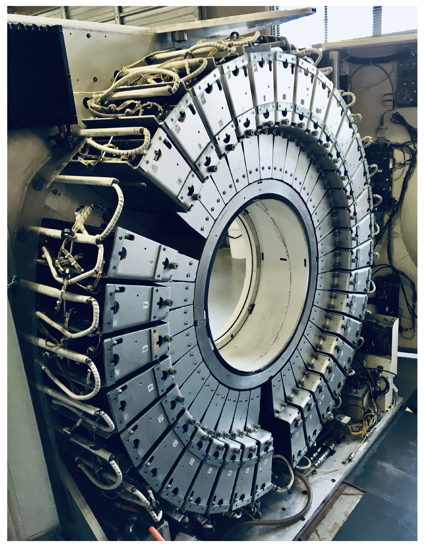
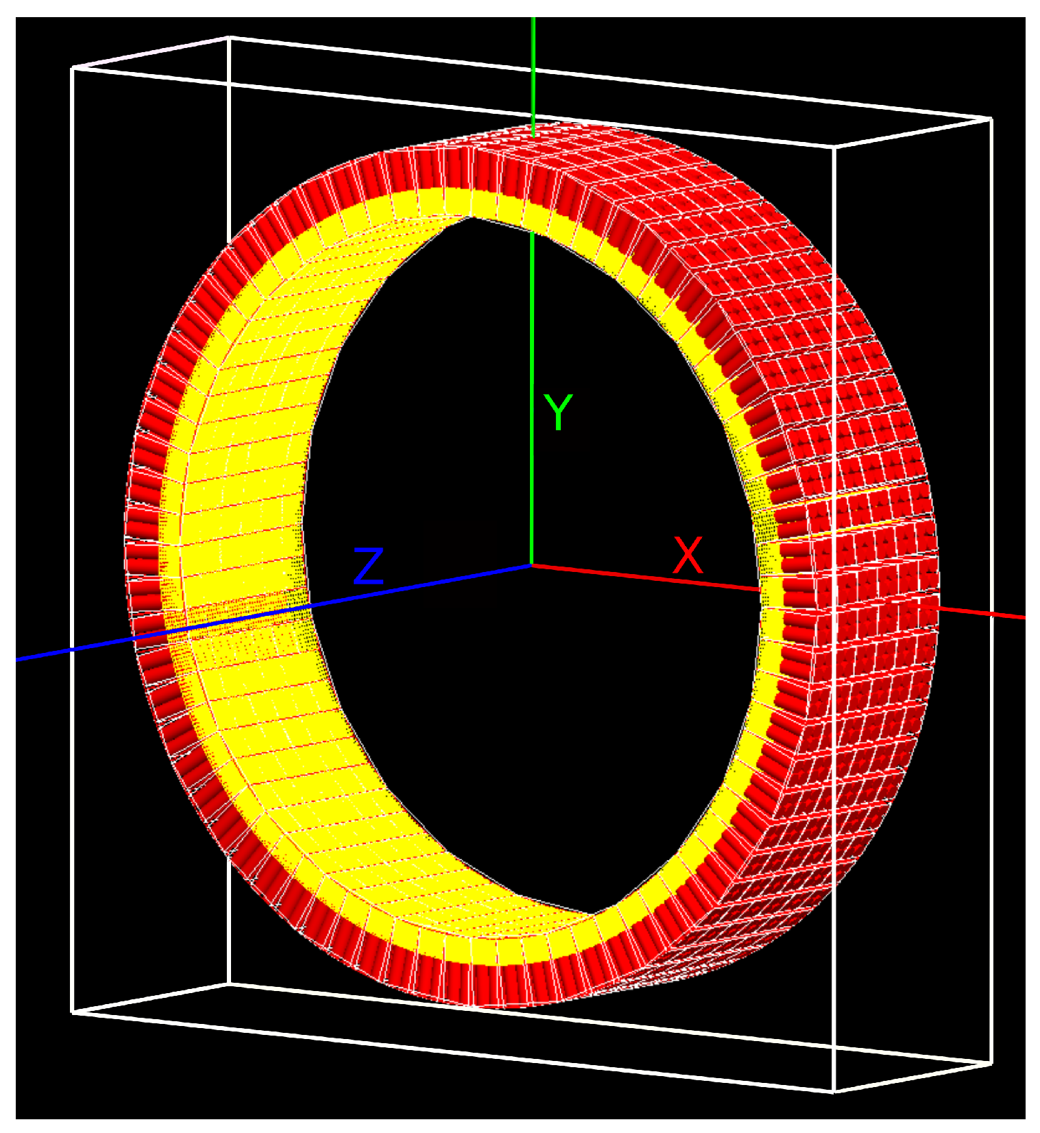
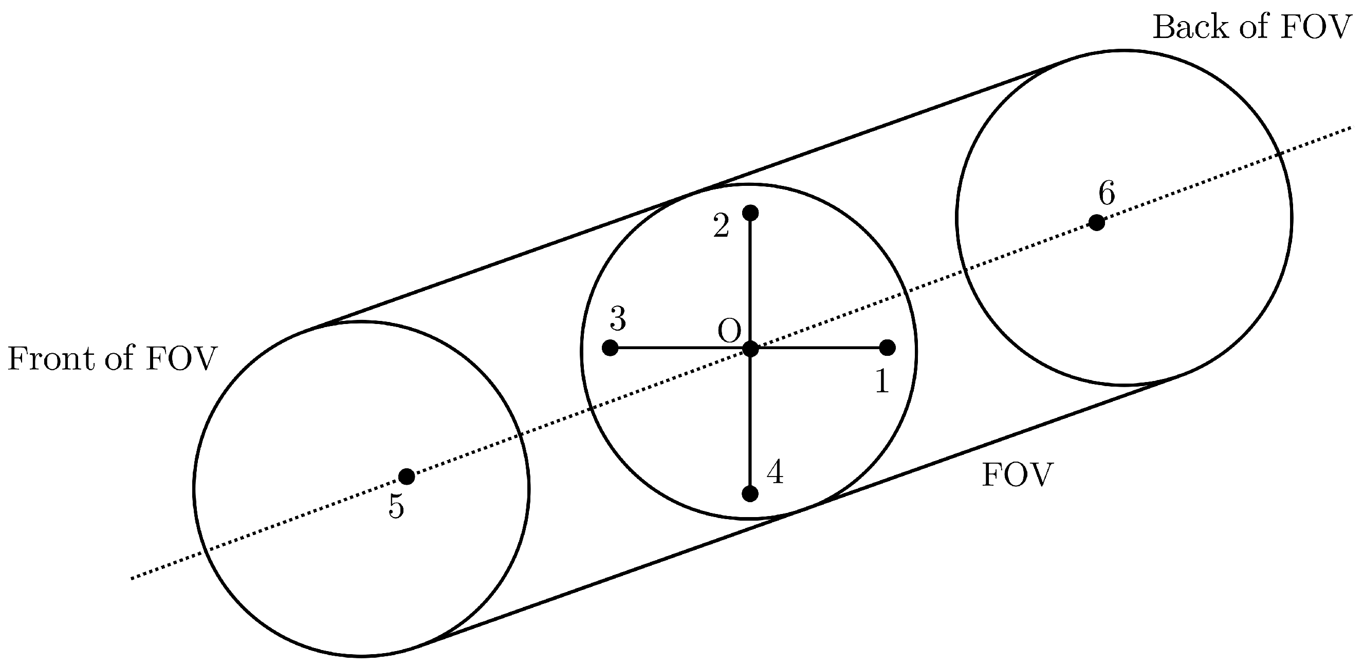
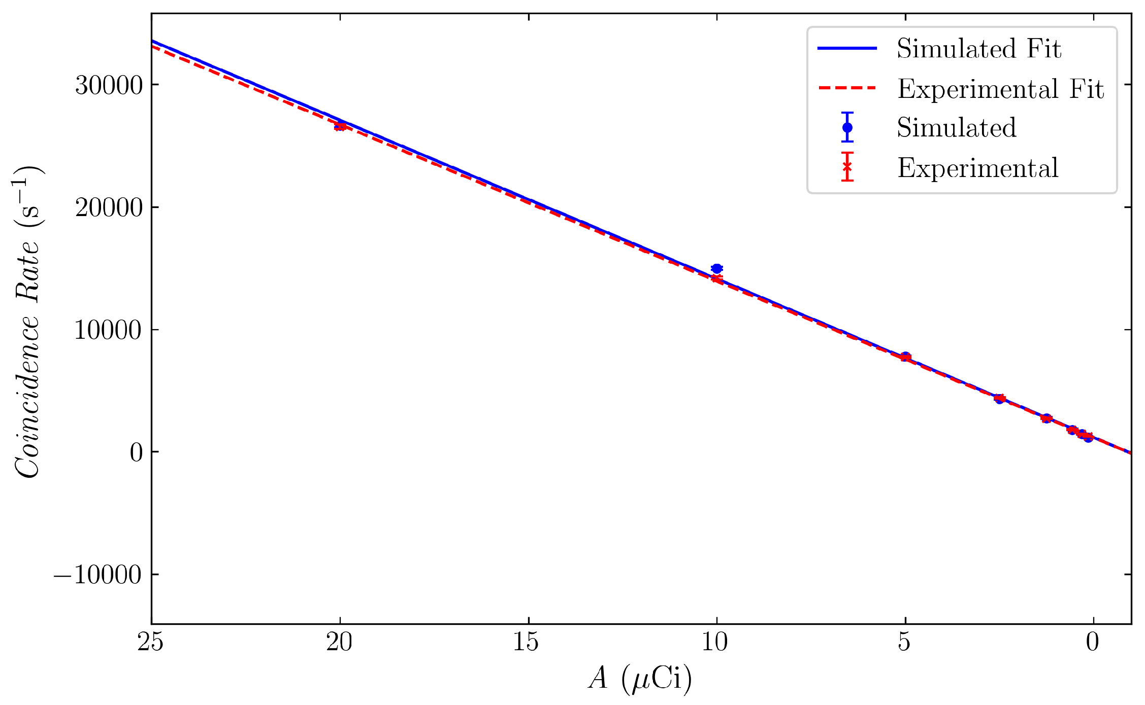
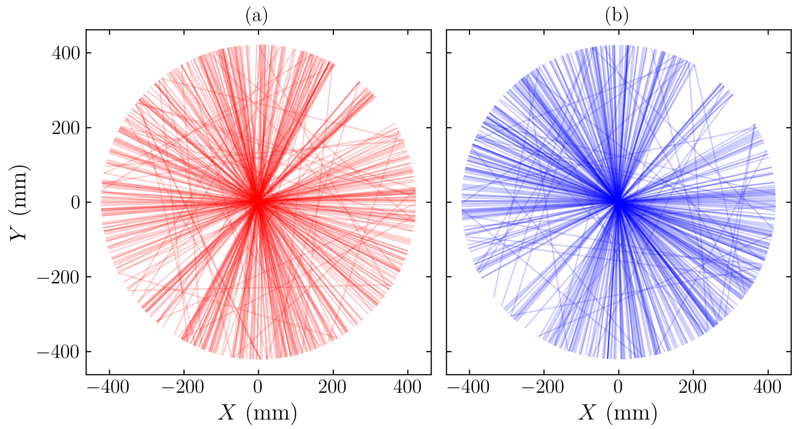
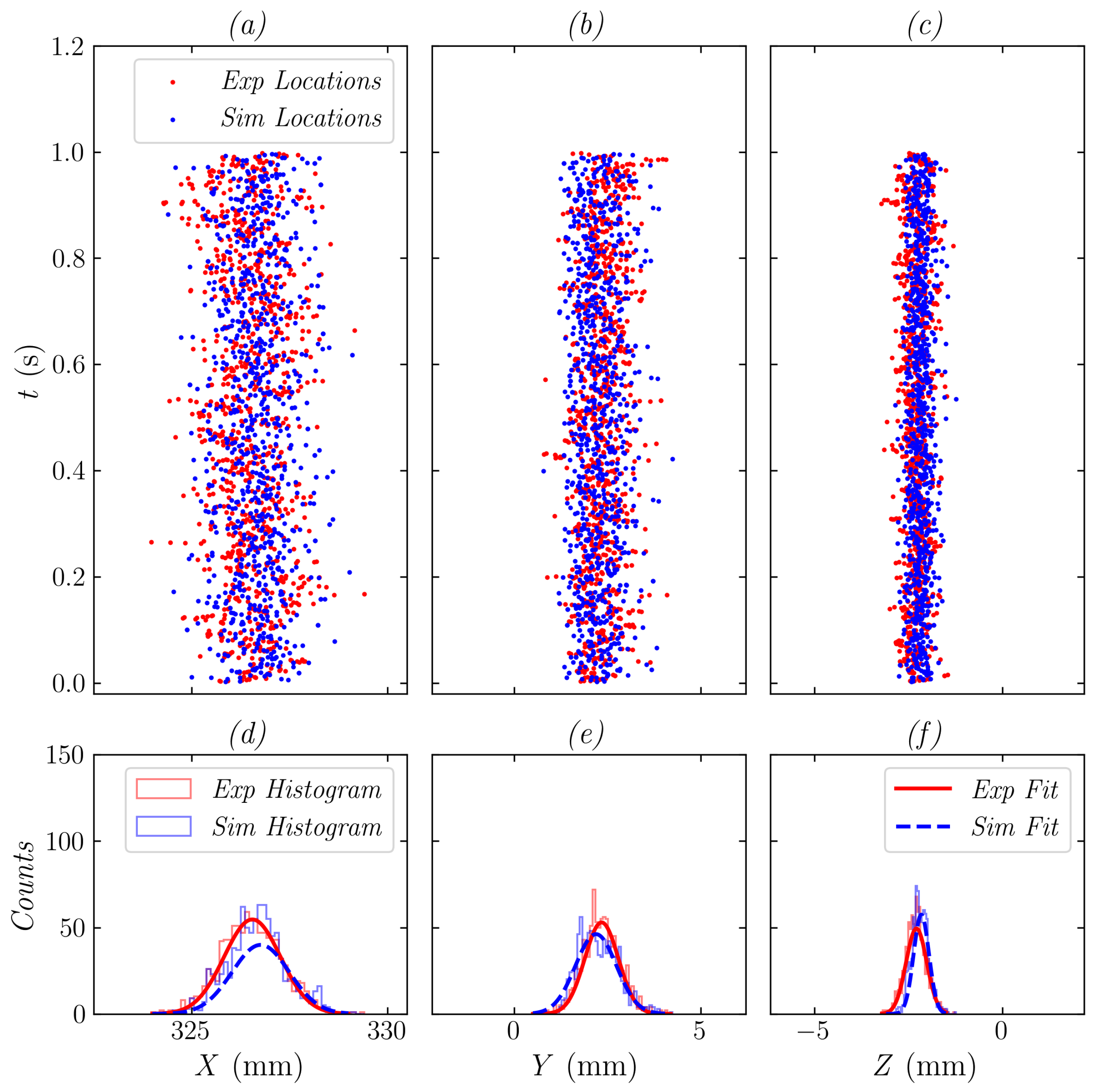
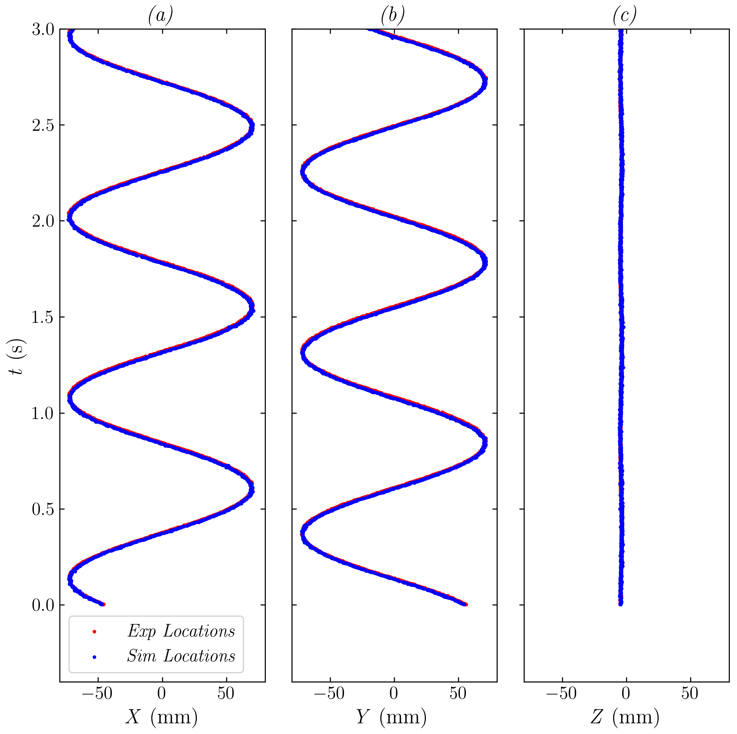
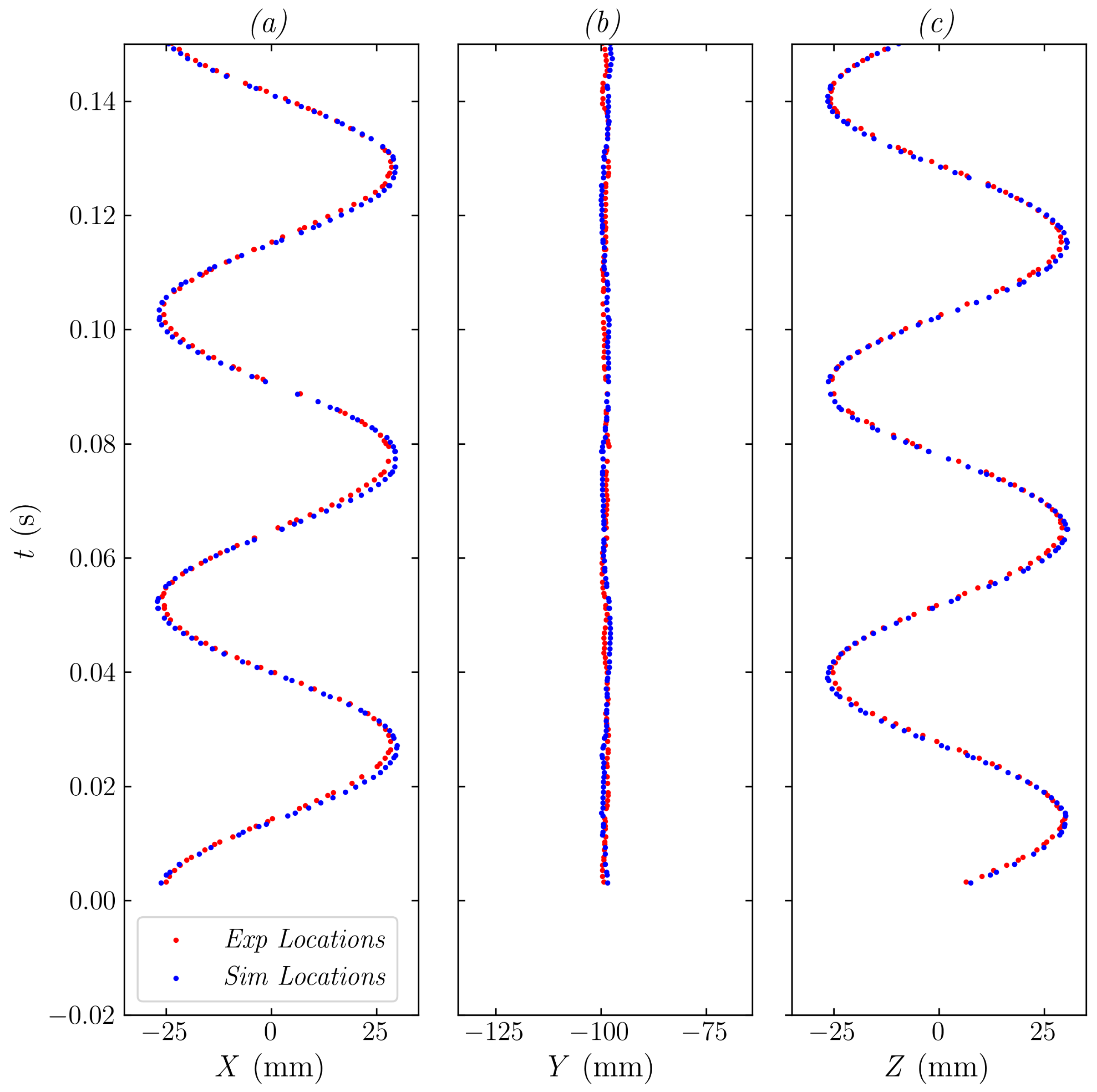
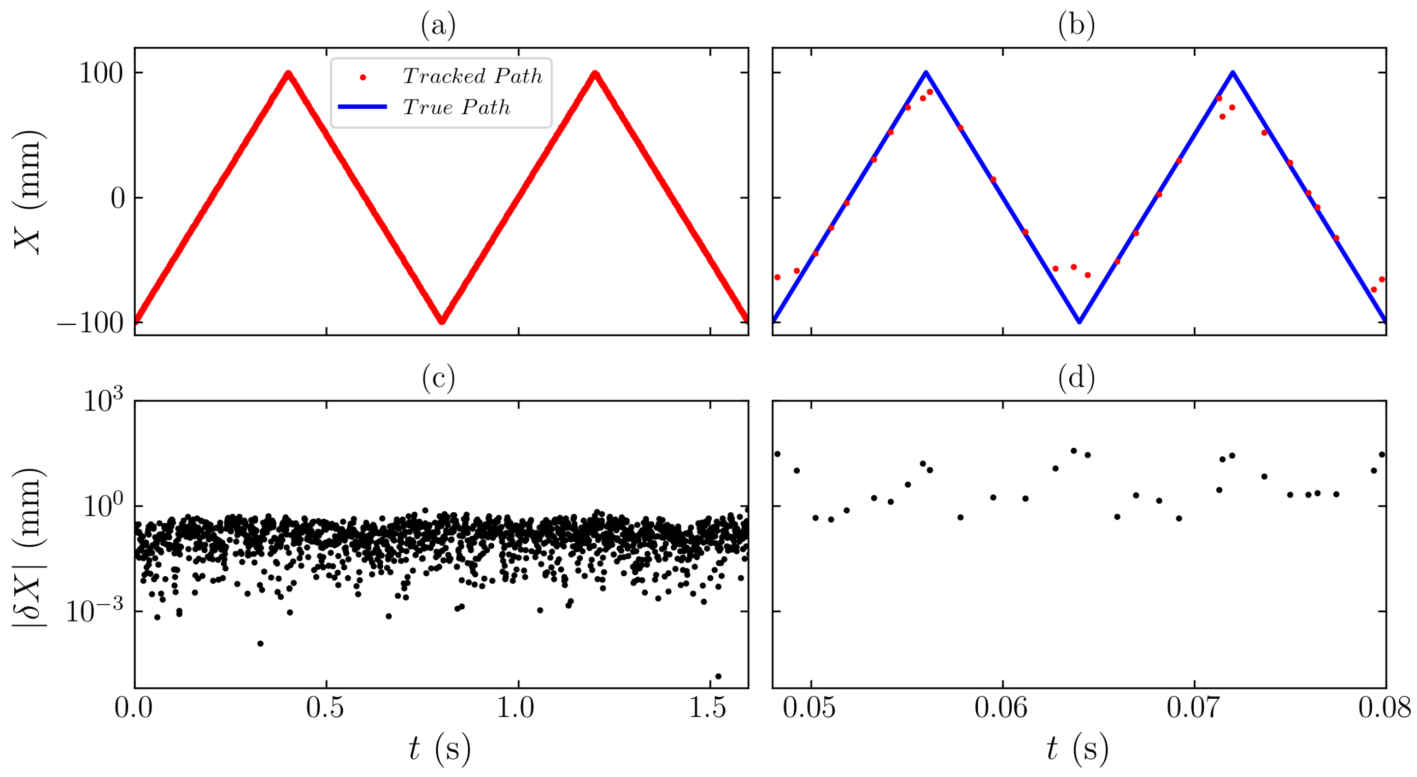
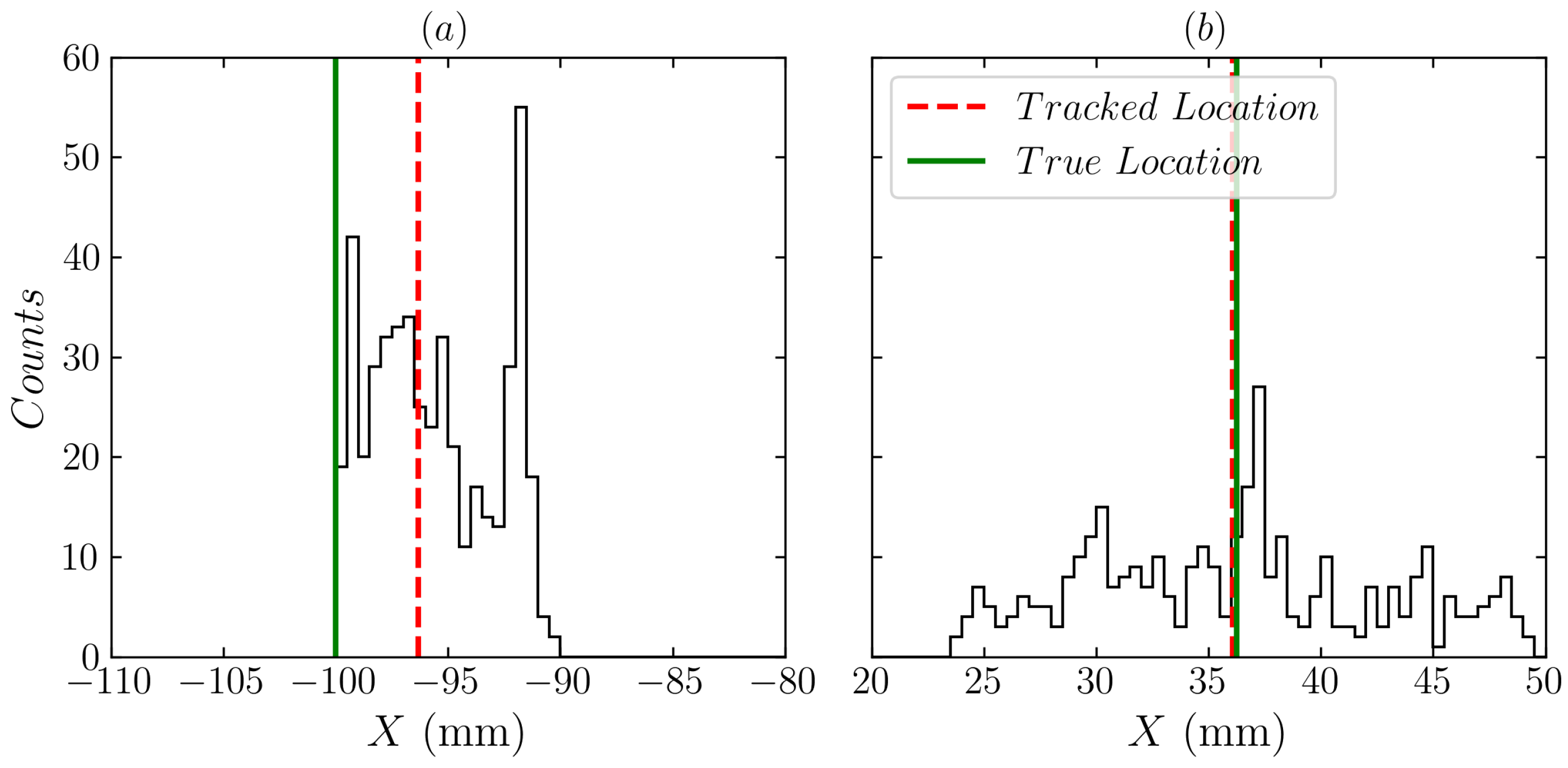
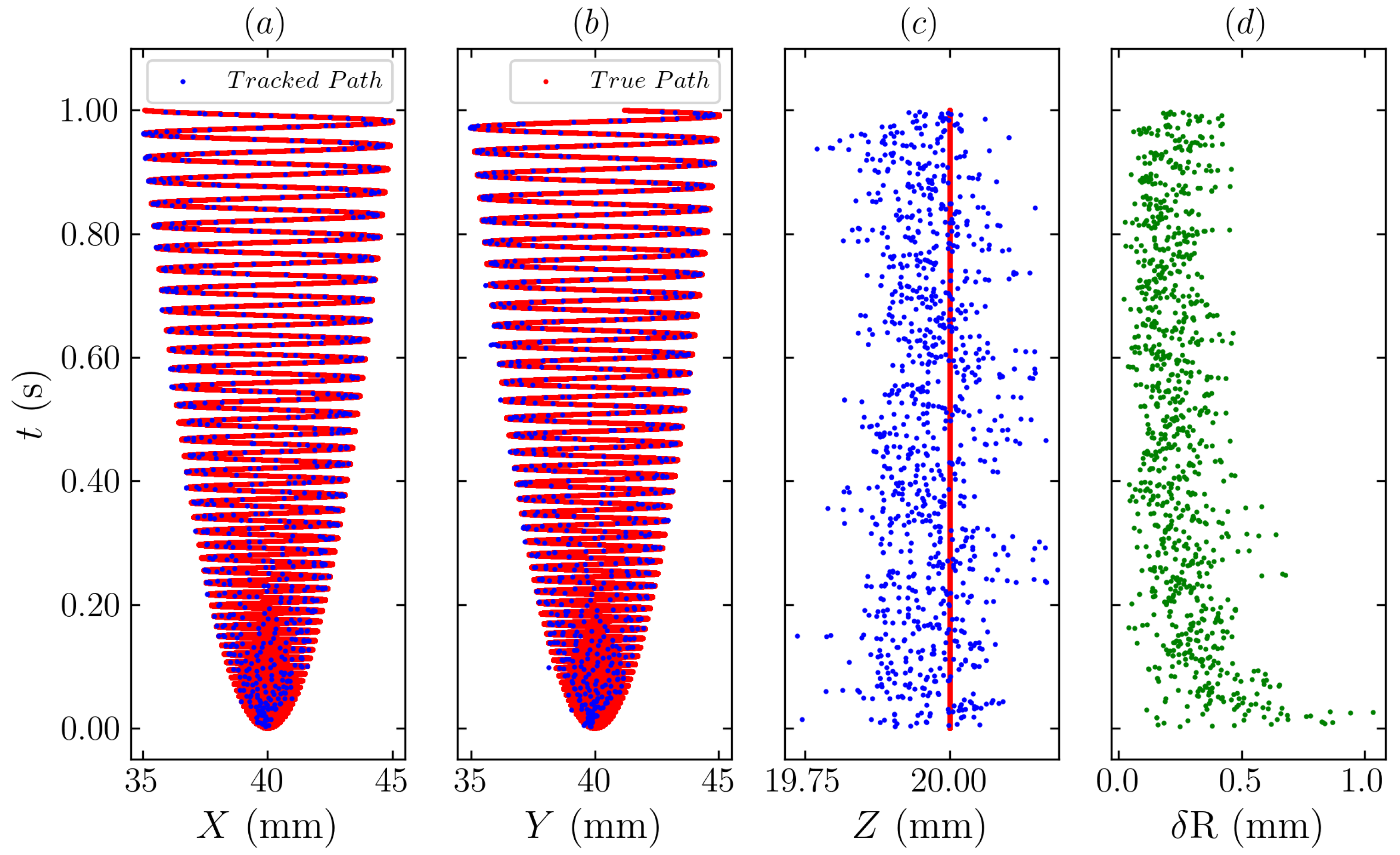
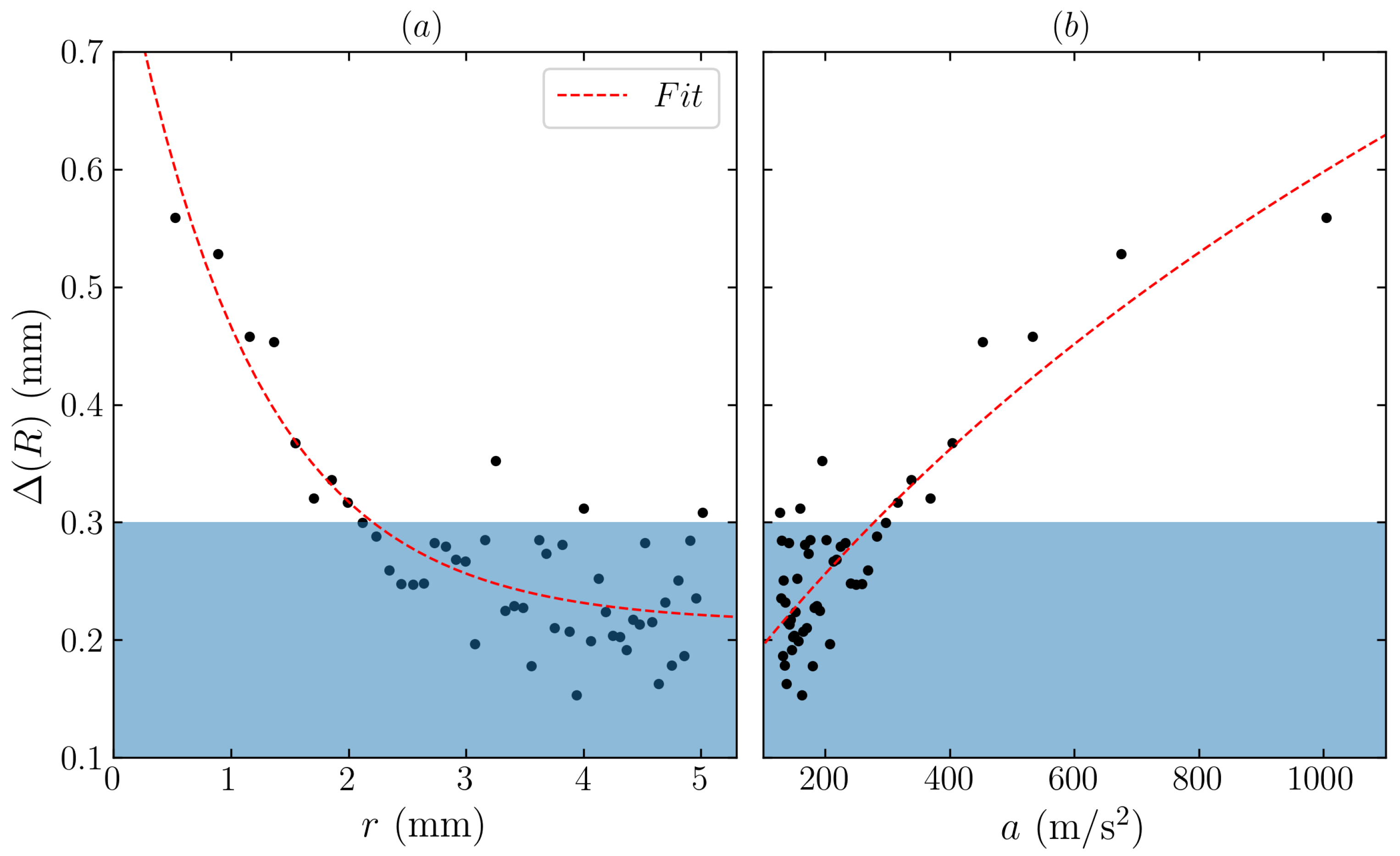
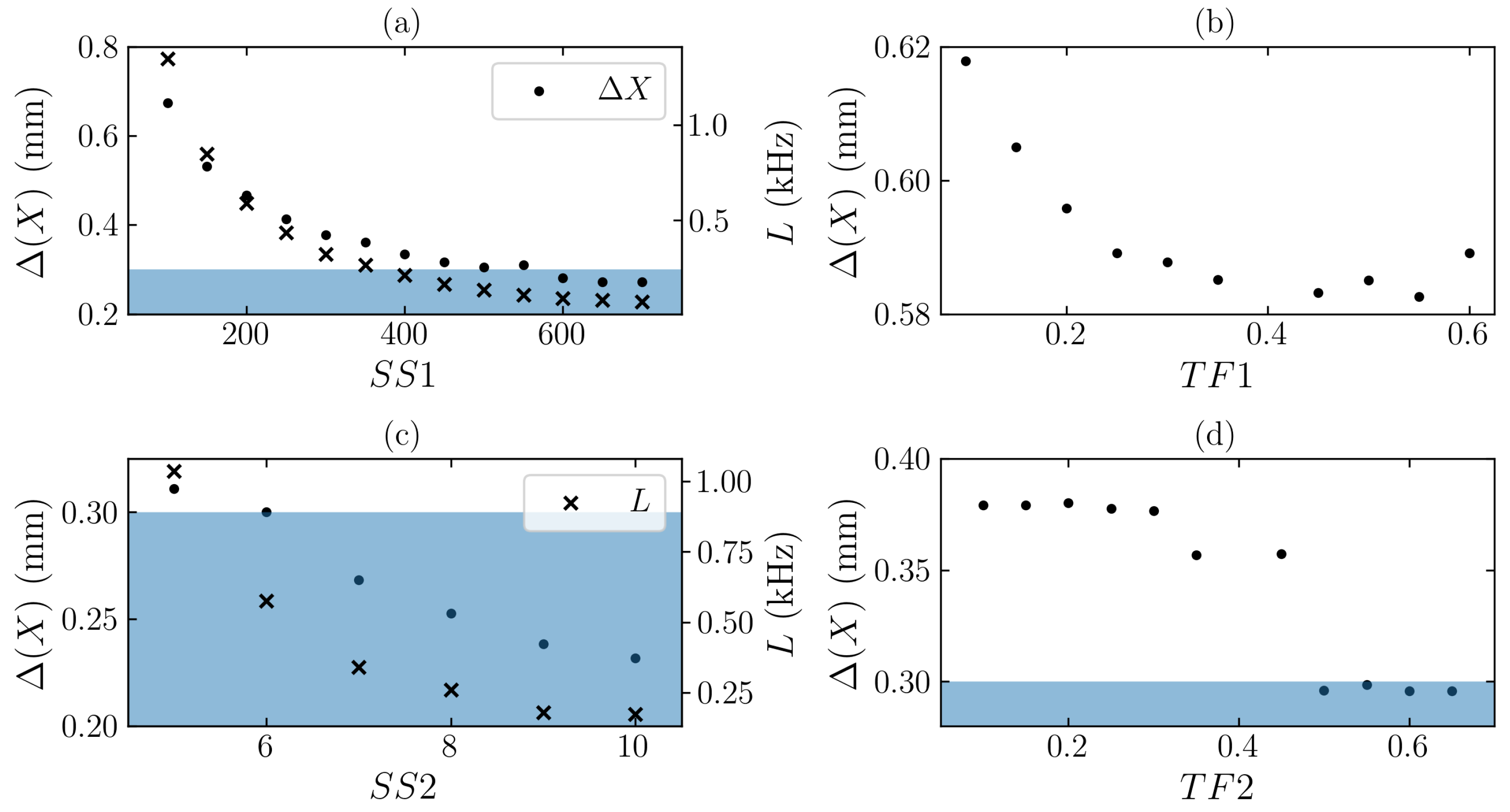
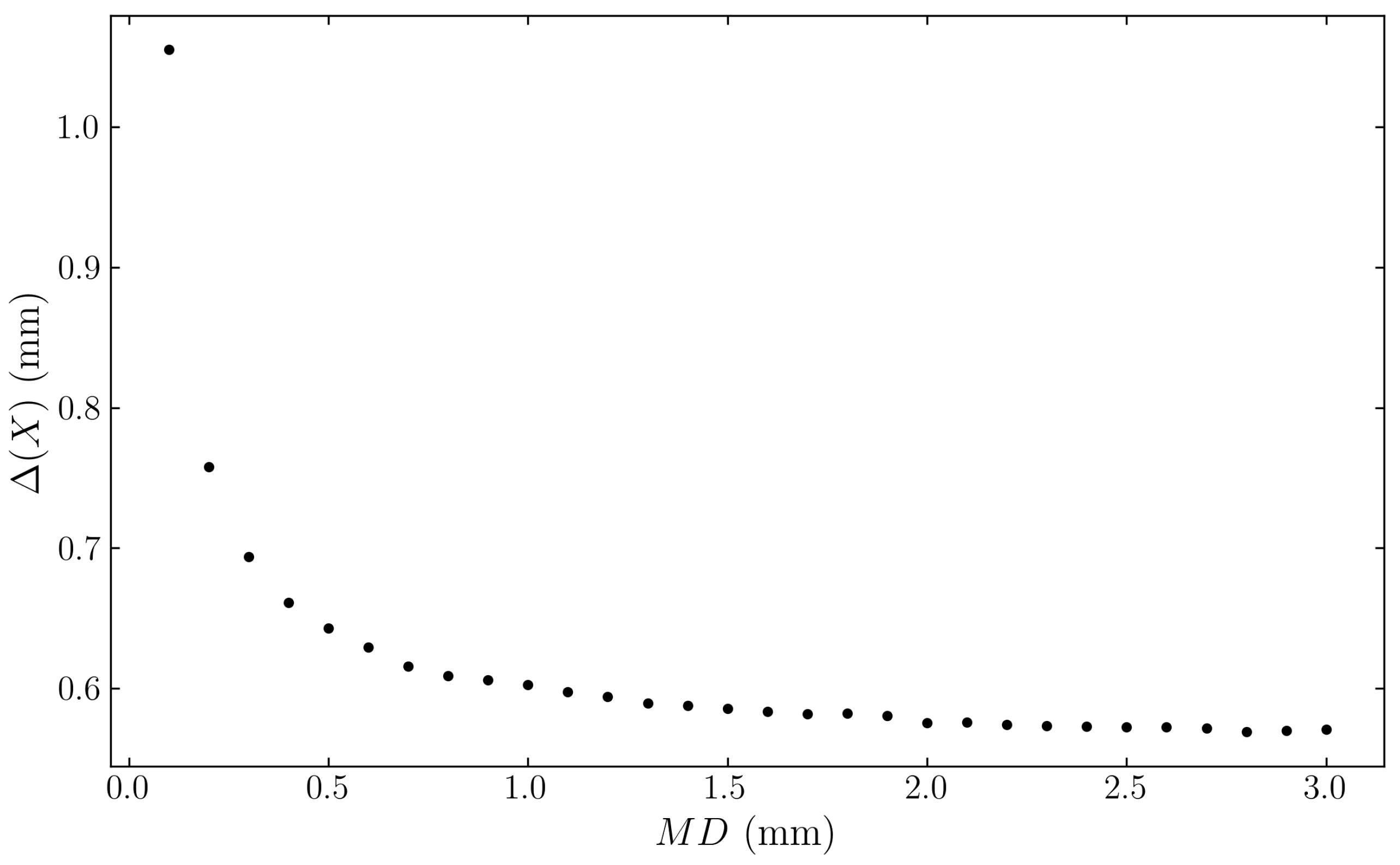
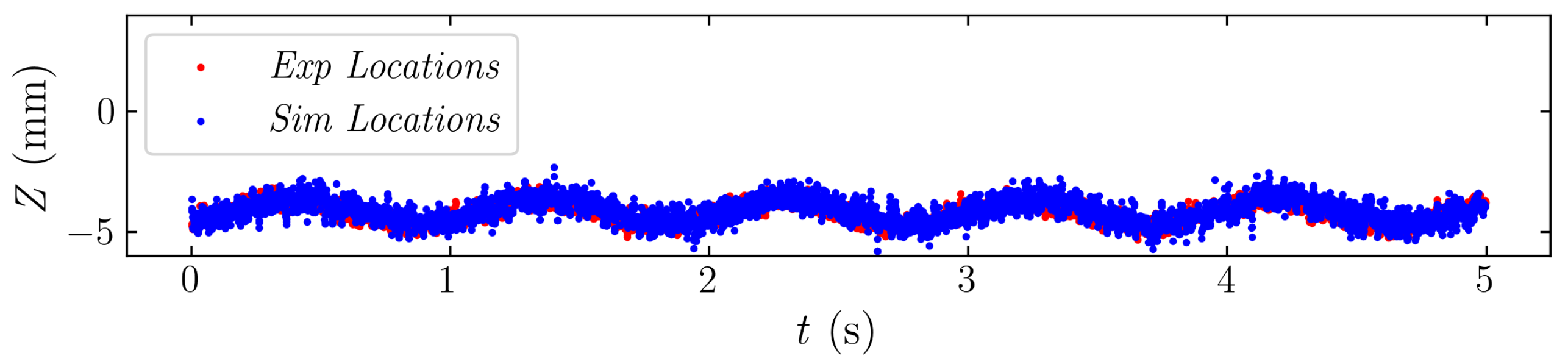
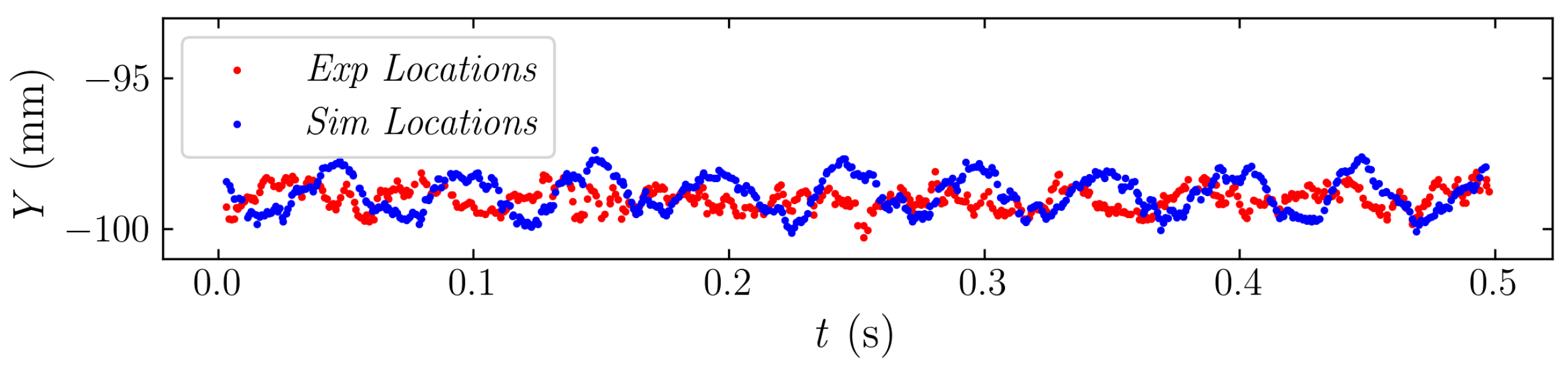


