An Intelligent Measurement Method and System for Vehicle Passing Angles

Abstract

Vehicle passing angles are critical metrics for evaluating the geometric passability of vehicles. The accurate measurement of these angles is essential for route planning in complex terrain and in guiding the production of specialized vehicles. However, the current measurement methods cannot meet the requirements of efficiency, convenience and robustness. This paper presents a novel measurement method by building and measuring the point cloud of a vehicle chassis. Based on this method, a novel measurement system is designed and its effectiveness is verified. In the system, a wheeled robot acquires and processes data after passing underneath the vehicle. Then, we introduce a new approach to reduce the main sources of error when building point clouds beneath the vehicle, achieved by modifying the extraction algorithm and the proportion of different feature points in each frame. Additionally, we present a fast geometric calculation algorithm for calculating the passing angles. The simulation experiment results demonstrate deviations of 0.06252%, 0.01575%, and 0.003987% when comparing the calculated angles to those of the simulated vehicle. The experimental results show that the method and system are effective at acquiring the point cloud of the vehicle and calculating the parameters of passing angles with good data consistency, exhibiting variances of 0.12407, 0.12407, and 0.69804.

1. Introduction and Background

Vehicle passing angles are important parameters in vehicle measurement standards [1]. The vehicle passing angles are the geometric parameters of a vehicle that determine a vehicle’s ability to pass on different terrains; the larger the passing angle, the better the ability to pass on steep roads. The stability- and quality-related measurements of vehicles’ passing angles affect the quality of acceptance in the industrial production of vehicles, and they also play an important role in the planning of transportation systems [2] and military deployment in complex terrains [3]. During the vehicle manufacturing process, the actual parameters often deviate from the designed vehicle model. Accurate measurements of these parameters are of significant importance for guiding production processes and determining competitive bidding. The vehicle passing angle diagram shown in Figure 1, which includes the approach angle, departure angle and ramp breakover angle [1], are still commonly measured manually in practice [4]. The staff must select the target points on the vehicle and estimate the position of the line tangent to the tire manually and then measure them and calculate the passing angles using trigonometric functions. However, this manual measurement method introduces multiple sources of error, making it inefficient and difficult to quantify and guarantee the consistency of the data and thus causing this method to be prone to controversy in both product acceptance and competitive bidding.

Existing automated non-contact measurement methods for vehicle contours are gradually maturing. A method for traversability assessment planning was proposed in the research of Zhang, K. et al. [5], which was based on the computation of a specific vehicle model considering the geometric information of a rough terrain surface obtained from laser scanning with LIDAR. However, this method mainly assesses the passability for a specific vehicle model and thus cannot be universally applied to vehicles easily or provide specific measurement parameters. Ma, Y. et al. [6] presented a measuring system that analyzes the wheels of passing vehicles using a horizontal LIDAR in a plane close and nearly parallel to the road surface. However, only the wheels were considered in the paper, and no data were collected from the chassis of the vehicle; thus, this method cannot be applied to calculate vehicle-related geometric parameters. In 2019, Xue, G. et al. [7] proposed another method to measure vehicle passing angles using a measuring plate and an improved tool instead of manual measurement. However, different models of modified lifting plates were required to fit the widely varying vehicle requirements, meaning that it is still a contact measurement method that needs to be more convenient. Some automated methods are available to measure the geometric parameters of vehicles [8,9,10,11]. However, these methods cannot be directly applied to the measurement of passing parameters. The methods proposed in [8,9,10] employ various image segmentation techniques combined with vehicle morphology [8], neural networks [9], or prior knowledge [10] to extract vehicle contour boundaries and calculate their dimensions. Although these single-view methods are fast, they tend to have larger errors, and they struggle to capture information about the vehicle’s bottom side using a single perspective. The method presented in [11] is a multi-view 3D imaging and detection approach that uses unmanned aerial vehicles to capture vehicle images from different angles and reconstruct them in 3D. However, these multi-view methods require comprehensive information from multiple angles to ensure robustness and accuracy. When capturing images of the vehicle’s bottom side, the angles of acquisition are limited, and factors such as lighting conditions and image quality can significantly affect the imaging quality and completeness. Additionally, the scale of the 3D models obtained using the Multi-View Stereo (MVS) approach needs to be adjusted to match real-world dimensions through camera-to-world scaling, introducing additional sources of error.

Laser scanning is a convenient, non-contact detection method with advantages including the ability to scan millions of points rapidly and detect some areas that traditional tools cannot cover. Due to these advantages, laser scanning has become popular, and its application has extended into the field of monitoring, detection, and identification. Luo, R. et al. [12] proposed a method to compare the daily construction scaffold technique using LIDAR point clouds. Point clouds were also applied to detecting changes in confined building interiors [13] and for automated damage detection and evaluation in bridges [14]. Njaastad, E.D. et al. [15] also adopted this method to identify geometric design parameters of ISO 484-class propeller blades using scanned point-cloud data. Laser point clouds can directly represent the geometric information of objects and can be used for measurement and evaluation. An empirical study on LIDAR point density [16] analyzed the variation across different land covers, providing a reference for a convenient approach to land classification. Researchers have also presented a method to evaluate the geometry of structures in underground mining based on LiDAR/Terrestrial Laser Scanner measurements [17]. The laser point cloud was also utilized to analyze the geometrical consistency of 3D-printed, cement-based materials with an as-designed modeled system [18].

Building point clouds is the foundation for measurements based on laser scanning. Scanning and registering point clouds using LIDAR is a universal point-cloud acquisition technique [19]. Many researchers have focused on how to build high-quality overall point clouds using different methods. An improved ICP algorithm was adopted by Liu, J. et al. [20] that used a corresponding accelerated method for point-cloud registration. Zhang, J. [21] proposed a state-of-the-art open source method that builds an overall point cloud in real time by dividing feature points and registering them separately. Shan, T and Englot, B. [22] presented a registration method with point segmentation to reduce grass interference. Principal component analysis was also used [23] to robustly extract features and build point clouds. Image information can complement some blind areas of laser scanning. The literature [24] presented better reconstructed 3D models by using laser scanning and photogrammetric data. Additionally, a more robust method [25] has been proposed using complement visual odometry to laser data.

Manual measurement of passing angles requires several staff and tools to cooperate, resulting in high labor costs and low efficiency. The target points selected based on manual experience often deviate due to the various components on the vehicle chassis, and the selected area is sometimes not a regular plane. The deviations are magnified by the angle conversion, leading to poor data consistency in repeated testing by different staff, causing disputes between evaluated companies during competitive bidding. An automated approach to measuring passing angles based on laser scanning can improve the efficiency and robustness of the measurement and reduce potential disputes. However, based on long-term field measurements, we still found it difficult to conveniently obtain the relevant point cloud through existing technical means due to differences in the scanning scenarios. The relevant point cloud includes the point cloud of the vehicle chassis and the point cloud of the tires below the chassis. In this scenario, the height of the LIDAR that can pass underneath the vehicle is low, limiting the field of view (FOV) of the LIDAR. During laser data acquisition, there is a large number of laser points on the flat ground. Moreover, the feature points that effectively represent the structure under a vehicle are sparse. These situations result in a much smaller proportion of vehicle chassis and tire point clouds in each frame of the laser data compared to ground point clouds, causing a disproportionate contribution of ground points in the alignment process. Additionally, the point cloud of the flat plane is more susceptible to the noise and vibration from the acquisition equipment, leading to odometry drift [26]. Furthermore, the ground points collected by the LIDAR near the flat ground present multiple circular shapes, and the alignment of circular-shaped point clouds is more likely to result in local optimal solutions, leading to alignment errors and mistakes. Consequently, it becomes challenging to obtain a reliable overall point cloud of the vehicle chassis and tires and even more challenging to obtain passing angle parameters with good data consistency based on that point cloud.

This paper proposes a method and designs a system that can be readily deployed to measure vehicle passing angles objectively, efficiently and robustly. Our system utilizes a wheeled robot equipped with a LIDAR and a camera to pass underneath the vehicle, scan and building the point cloud and calculate the passing angles automatically. In our method, we propose a novel point cloud-building approach to address the challenges of building point clouds from underneath a vehicle and a point cloud-based parameter measurement approach to select target points and measure passing angles without the use of manual operations.

This article is organized as follows: Section 2 describes the system, Section 3 details the method, Section 4 presents the experimental results, Section 5 provides a discussion of the proposed system and Section 6 concludes this article.

2. Design of the Measurement System

The primary challenge in efficiently automating the measurement of vehicle passing parameters is how to obtain data from underneath the vehicle without modifying the testing site or the testing platform. To address this issue, we propose a solution involving a wheeled robot equipped with sensing devices that passes underneath the vehicle. Subsequently, a three-dimensional point cloud is built and the parameters are calculated based on the data extracted from the point cloud. The schematic diagram in Figure 1 illustrates the operation of the passing angle measurement system. In this system, the wheeled robot equipped with a LIDAR and a camera longitudinally passes underneath the vehicle to acquire the data on the vehicle chassis, tires and the ground. The overall point cloud is built by the processor and subsequently analyzed to derive the passing angles. The final results are transmitted to the handheld device to be recorded and displayed.

2.1. Hardware System Framework

For the convenience of system operation, the measurement system consists of measurement equipment and an operator interface. The operator interface is a handheld device used to initiate and terminate the system and to receive the point cloud data and calculated parameter data processed by the industrial PC mounted on the wheeled robot. As shown in Figure 2, the hardware block includes a wheeled robot and a handheld device. The wheeled robot’s dimensions are 295 mm in width, 384 mm in length and 88 mm in height, while the LIDAR has a diameter of 103 mm and a height of 72 mm. The system is suitable for common household vehicles, off-road vehicles, delivery vehicles and any special vehicle with a chassis higher than 160 mm.

In the robot, the STM32 is used as the controller for its actuator, which controls the motor system to drive the McNamee wheel to achieve movement via the CAN bus and electronic speed controller (ESC). The wheeled robot can move in all directions without rotating. In such a case, the motion model of the equipped LIDAR can be considered as a linear model [27], simplifying the distortion correction problem caused by the LIDAR data’s width moving.

The LIDAR used in our system is a VLP-16, which has a 16-channel laser sensor distributed over a vertical FOV of 30° (±15°) and an angular resolution of 2°. The camera selected in our system is the RealSense D435.

The digital transmission and receiver units access a handheld PC and the industrial PC via USB universal ports for communication to facilitate remote start-up and interrupt control.

Regarding the placement position of the LIDAR, if the Z-direction is oriented towards the front of the wheeled robot, both the vehicle and the ground are too close to the sensor, causing interference in obtaining the point cloud data. Therefore, the LIDAR is horizontally positioned on the wheeled robot horizontally, as shown in Figure 1. This configuration allows the laser lines above the horizontal line of the LIDAR to gradually scan the vehicle chassis and a portion of the tires as the wheeled robot moves.

2.2. Software System Overview

An overview of the software framework is shown in Figure 3.

The overall system is divided into three modules. The first module, data acquisition, involves receiving and processing the raw data acquired by the camera and the LIDAR to obtain the odometry. The second module, point cloud building, constructs a feature map based on the odometry and the feature points, estimating the pose through a scan-to-map algorithm [28]. The estimated pose is then used to fuse all point cloud frames. The third module, parameter calculation, obtains passing angles by selecting and calculating the target point at the overall point cloud automatically. Section 3 describes the details of the software system’s algorithms.

3. Measurement Method

3.1. Segmentation

When acquiring point clouds from underneath vehicles, a significant portion of the points often corresponds to the ground. The circular shape of the ground point cloud can introduce matching errors between point cloud frames and increase the likelihood of encountering local optima. To address this issue, we employ the RANSAC (random sample consensus) algorithm [29,30] to remove the ground points in each frame based on point features, thereby enhancing the quality of the point clouds. Both sphere and plane features can be utilized for point cloud frames, as the ground points form a circular shape on a plane in a single frame. Based on experimental results concerning efficiency and time consumption, we choose the plane model to select inliers for the RANSAC algorithm. In this section, our objective is to reduce the number of ground points quickly, allowing us to halt the iteration when the number of inliers exceeds 50% of the point cloud in the frame and then segment these inliers from the frame.

3.2. Motion Compensation

In our method, data compensation is necessary to account for the movement speed of the wheeled robot, as the laser scan is prone to distortion while the robot is in motion (Figure 4). When the wheeled robot moves linearly, the LIDAR moves at a constant linear velocity, while its internal laser sensor is scanning at constant angular velocity. In such case, the motion compensation problem can be simplified.

The $0^{°}$ of the LIDAR is aligned with the moving direction of the wheeled robot under ideal conditions, as shown in Figure 4. In actual conditions, the installation deviation angle $A$ and the actual motion speed $v$ of the wheeled robot can be obtained through system calibration. Therefore, the points in each frame can be compensated as:

$$\left\{\begin{array}{c}{x}_i=x_i^0-\alpha v\frac{\theta }{{\omega }_{\mathrm{r}}}\sin (A)\\ \begin{array}{l}{y}_i=y_i^0+\alpha v\frac{\theta }{{\omega }_{\mathrm{r}}}\cos (A)\\ z_i=z_i^0\end{array}\end{array}\right.$$

(1)

where ${\omega }_r$ is the rotation speed of the laser sensor inside the LIDAR, $\theta$ is the LIDAR’s angle of rotation, $(x_i^{},y_i^{},z_i^{})$ are the coordinates after compensation, and $\alpha$ is the experience scaling factor.

3.3. Laser Odometry

In this paper, laser odometry is calculated based on the 3D point cloud data obtained from the LIDAR, while visual odometry is calculated using feature points extracted from the 2D image. The odometry, which exhibits smoothness, is obtained from both of them.

Laser odometry is computed by extracting and aligning feature points from each point cloud frame, following a similar approach as described in [21,22], where corner points and plane points are differentiated based on the point curvature for alignment. In this study, the feature point extraction has been improved to cater to the measurement task in this part.

Outliers refer to sparse points located at a certain distance from the main structure of the point cloud. Outliers are typically caused by insufficient scanning coverage or noise, etc. During the extraction of corner points, outlier points can easily be detected as corner points by the computer. However, these outlier points do not accurately represent the structure of the scanned object and can introduce negative interference, affecting both the accuracy and precision of the alignment process. Therefore, it is necessary to remove outlier points in each frame during the feature extraction in our measurement task.

Since the laser point cloud in a single frame is distributed along 16 laser lines, all points can be processed along these laser lines. In this section, for point cloud feature extraction and outlier points determination, a sliding window $W$ is employed in each laser line. Each point is considered as the center point within the sliding window, and $N$ adjacent points are selected for calculation.

The constraint on the length of sliding window $W$ is calculated as:

$$r_w=\left|\arcsin (\frac{y_N}{\sqrt{x_N^2+y_N^2}}-\frac{y_{-N}}{\sqrt{x_{-N}^2+y_{-N}^2}})\right|$$

(2)

where $r_w$ represents the length constraint of $W$, which is the angle between the first and last points in the window in the LIDAR coordinate system $L$.

The width of $W$ is limited to $r_w<1/16\pi$, and any point that exceeds this limit will not be counted or processed.

The average distance from the center point to the other points in $W$ is calculated as:

$$l_a=\frac{1}{2N}{\displaystyle \sum _{j=-N}^N{l}_j}$$

(3)

where

$$l_j=\sqrt{{(x_0^W-x_j^W)}^2+{(y_0^W-y_j^W)}^2+{(z_0^W-z_j^W)}^2},j\in [-N,N]$$

(4)

where $(x_0^W,y_0^W,z_0^W)$ is the center point. Then, the StatisticalOutlierRemoval filter [31] is applied to remove outliers.

The smoothness score for fast feature point extraction is also considered here. Different from the method in [21], the smoothness score is calculated simultaneously with the outlier points in the window to improve efficiency and eliminate outliers and unstable feature points that may cause interference. The smoothness score is defined as:

$$c=\frac{‖{\displaystyle \sum _{j=-N}^N[(x_j^W,y_j^W,z_j^W)-(x_0^W,y_0^W,z_0^W)]}‖}{\left|W\right|·‖(x_0^W,y_0^W,z_0^W)‖}$$

(5)

The points for which $c>{\lambda }_{c1}$ are considered corner feature points, and the points for which $c<{\lambda }_{c2}$ are considered plane feature points, where ${\lambda }_{c1}$ and ${\lambda }_{c2}$ are the corner feature threshold and the plane feature threshold, respectively.

The window used for outlier removal and feature extraction is constrained in such a way that allows the algorithm to avoid extracting points at the edge of structural fractures and outliers to some extent, as shown in Figure 5.

Finally, the two-step alignment method by Levenberg–Marquardt [21] is used in our method to obtain the laser odometry.

3.4. Odometry

The feature points of image frames are calculated as the wheeled robot passes underneath the vehicle, allowing for the estimation of visual odometry [32]. This visual odometry serves as a supportive component to the dominant LIDAR odometry, enhancing the alignment process by incorporating relevant vehicle data and reducing alignment errors.

The wheeled robots are programmed to move in a fixed direction at a constant speed. With this knowledge, the rotation and translation components can be processed separately. The rotation increment can be considered constant, while the translation increment can be approximated as uniform. Therefore, the knowledge of the motion constraint can be applied to the odometry to reduce the error in Algorithm 1.

Algorithm 1: Odometry

Input:  $\overline{d}$$, d_l^k$$, d_v^k$$, \Delta d_l^k$ Output:  $d_o^k=[Q_o^k,T_o^k]$

1: $\mathrm{if} \mathrm{the} \mathrm{elements} \mathrm{in} Abs(O_l^k)<[0.1,0.1,0.1]$ then 2:    $Q_o^k=Q_l^k$$\mathrm{The} Abs()$ refers to taking the absolute value of each element in the matrix. 3:  else 4:    $Q_o^k=\min \{Sum(Q_l^k),Sum(Q_v^k)\}$$\mathrm{The} Sum()$ refers to summing the elements in the matrix. 5: end if 6: $\mathrm{if} \mathrm{the} \mathrm{elements} \mathrm{in} Abs(T_l^k)<[0.1,0.5,0.1]$ then 7:    $T_o^k=T_l^k$ 8:  else 9:    $T_o^k=\min \{Sum(T_l^k),Sum(T_v^k)\}$ 10:  end if 11:  $\mathrm{return} d_o^k=[Q_o^k,T_o^k]$

The averaged odometry data from the previous ten instances of approximately uniform motion are used as a reference value as follows:

$$\overline{d}=\frac{1}{10}{\displaystyle \sum _{p=1}^{10}\frac{1}{2}}(d_l^p+d_v^p)$$

(6)

where $d_l^p$ and $d_v^p$ denote the laser odometry and visual odometry of the $p$ frame, respectively.

Then, the variation in the odometry at $k$ time is obtained as follows:

$$\left\{\begin{array}{c}\Delta d_l^k=d_l^k-\overline{d}\\ \Delta d_v^k=d_v^k-\overline{d}\end{array}\right.$$

(7)

where $d_l^k=[Q_l^k,T_l^k]$, $\Delta d_l^k=[\Delta Q_l^k,\Delta T_l^k]$, $d_v^k=[Q_v^k,T_v^k]$ and $\Delta d_v^k=[\Delta Q_v^k,\Delta T_v^k]$. Here, $Q=[q_x,q_y,q_z,q_w]$ denotes the component of the rotation and $q_x,q_y,q_z,q_w$ are the quaternions. $T=[x_T,y_T,z_T]$ denotes the component of the translation.

Therefore, the odometry $d_o^k$ at $k$ time is obtained by combing laser odometry and visual odometry according to the constraints.

3.5. Point Cloud Building

In this section, the odometry and the features of the plane and corner are utilized to create a feature point map. The feature points of the subsequent frames are aligned with the feature point map [28] to estimate the pose [30]. The LIDAR point cloud frames are fused based on the estimated pose to build an overall point cloud. To reduce noise while preserving the edges, bilateral filtering [31,33] is applied.

3.6. Parameter Calculation

After building the point cloud, it is necessary to align it with national regulations to identify target points and calculate the parameters. Several parameters of vehicle chassis can be calculated rapidly by rotating and segmenting the overall point cloud collected by this paper. Here, we focus on solving the passing angles, which currently have the lowest degree of automated detection and the poorest data consistency in Algorithm 2.

Algorithm 2: Parameters calculation

Input: L1, L2, L3, T1, T2 Output: $\alpha$, $\beta$, $\lambda$

1: Select a point $A_o$$\mathrm{in} \mathrm{L}1 \mathrm{and} \mathrm{a} \mathrm{point} B_o$ in T1 as init. 2: $\mathrm{for} \mathrm{traverse} \mathrm{the} \mathrm{point} A_o$ in L1 do 3:    $\mathrm{Choose} \mathrm{the} \mathrm{point} A$ so that it satisfies Equation (8). 4: end for 5: $\mathrm{for} \mathrm{traverse} \mathrm{the} \mathrm{point} B_o$ in T1 do 6:    $\mathrm{Choose} \mathrm{the} \mathrm{point} B$ so that it satisfies Equation (9). 7: end for 8: $\mathrm{Calculate} \mathrm{the} \mathrm{approach} \mathrm{angle} \alpha$ as Equation (10). 9: $\mathrm{Select} \mathrm{a} \mathrm{point} G_o$$\mathrm{in} \mathrm{L}3, \mathrm{and} \mathrm{a} \mathrm{point} F_o$ in T2 as init. 10:  $\mathrm{for} \mathrm{traverse} \mathrm{the} \mathrm{point} G_o$ in L3 do 11:    $\mathrm{Choose} \mathrm{the} \mathrm{point} G$ so that it satisfies Equation (11). 12:  end for 13:  $\mathrm{for} \mathrm{traverse} \mathrm{the} \mathrm{point} F_o$ in T2 do 14:    $\mathrm{Choose} \mathrm{the} \mathrm{point} F$ so that it satisfies Equation (12). 15:  end for 16:  $\mathrm{Calculate} \mathrm{the} \mathrm{departure} \mathrm{angle} \lambda$ as Equation (13). 17:  $\mathrm{Select} \mathrm{a} \mathrm{point} C_o$$\mathrm{in} \mathrm{L}2, \mathrm{a} \mathrm{point} D_o$$\mathrm{in} \mathrm{T}1 \mathrm{and} \mathrm{a} \mathrm{point} E_o$ in T2 as init do 18:    $\mathrm{for} \mathrm{traverse} \mathrm{the} \mathrm{point} C_o$ in L2 do 19:      $\mathrm{Choose} \mathrm{the} \mathrm{points} D_p$$\mathrm{and} E_p$ so that it satisfies Equation (14). 20:    end for 21:    $\mathrm{Calculate} \mathrm{angle} {\beta }_o$ as Equation (16). 22:    $\mathrm{if} {\beta }_o$ is minimum then 23:      $\mathrm{Calculate} \mathrm{the} \mathrm{ramp} \mathrm{break} \mathrm{angle} \beta ={\beta }_o$, as Equation (15). 24:    end if 25:  end for 26:  $\mathrm{return} \alpha$, $\beta$, $\lambda$

An iterative algorithm is employed to determine the target points during the calculation of passing angles, as shown in Figure 6. The point cloud belonging to the vehicle body and the point clouds associated with the tires are separated using the RANSAC method, which utilizes a planar model for the body and a cylindrical model for the tires. Subsequently, these point clouds are projected onto suitable surfaces for further analysis.

The cylindrical model is used to segment the tire point clouds, allowing for the extraction of parameters such as the circle center and radius. Additionally, based on these parameters and the Z-axis coordinates, the lower portion of the tire point clouds, referred to as T1 and T2, can be extracted to reduce computational overhead. Similarly, the body point cloud can be segmented into LI, L2 and L3 using these parameters. The approach angle, ramp break-over angle and departure angle are then calculated according to the standard definition [1].

In Algorithm 2, certain points should be selected randomly. As shown in Figure 6, points $B_o$, $D_o$, $E_o$ and $F_o$ represent the initial random selection points in the edge part of the tire point clouds. Additionally, points $A_o$, $G_o$ and $C_o$ represent the traversal points in the point cloud of the body.

The target point $A$ for the approach angle can be obtained by traversing as:

$$\frac{z_A-z_{B_o}}{y_A-y_{B_o}}=\min \left\{\frac{z_{A_o}-z_{B_o}}{y_{A_o}-y_{B_o}}\right\}$$

(8)

Another target point for the approach angle is $B$, that is, the tangent point between the ray of the target point A and the tire. This tangent point can be found by traversing T1, where the line connecting T1 to the center of the tire is perpendicular to the line connecting T1 to point A. The process can be described as:

$$\left|\overrightarrow{B{O}_1}\times \overrightarrow{BA}\right|=0$$

(9)

Additionally, the approach angle can be obtained as:

$$\alpha =\arctan (\frac{z_A-z_B}{y_A-y_B})$$

(10)

The calculation of the departure angle is similar to that of the approach angle. The difference lies in traversing the L3 points and the rear tire point cloud T2. The process of finding the target point $G$ can be described as:

$$\frac{z_G-z_{F_o}}{y_G-y_{F_o}}=\min \left\{\frac{z_{G_o}-z_{F_o}}{y_{G_o}-y_{F_o}}\right\}$$

(11)

Additionally, we can find the other target point $F$ that satisfies:

$$\left|\overrightarrow{F_o{O}_2}\times \overrightarrow{F_{o}G}\right|=0$$

(12)

Finally, the departure angle is obtained by:

$$\beta =\arctan (\frac{z_F-z_G}{y_F-y_G})$$

(13)

The ramp break angle is obtained by traversing L2 and calculating the tangent points of the adjacent tires for each point in L2. For each point, the tire edge point clouds are traversed to find the tangent line as follows:

$$\left|\overrightarrow{D_p{O}_1}\times \overrightarrow{D_p{C}_o}\right|=\left|\overrightarrow{E_p{O}_2}\times \overrightarrow{E_p{C}_o}\right|=0$$

(14)

The ramp breakover angle can be obtained as follows:

$$\beta =\min \left\{{\beta }_o\right\}$$

(15)

where the ${\beta }_o$ is defined as follows:

$${\beta }_o=\arctan (\frac{z_{C_o}-z_{D_p}}{y_{C_o}-y_{D_p}})+\arctan (\frac{z_{C_o}-z_{E_p}}{y_{C_o}-y_{E_p}})$$

(16)

4. Experiment

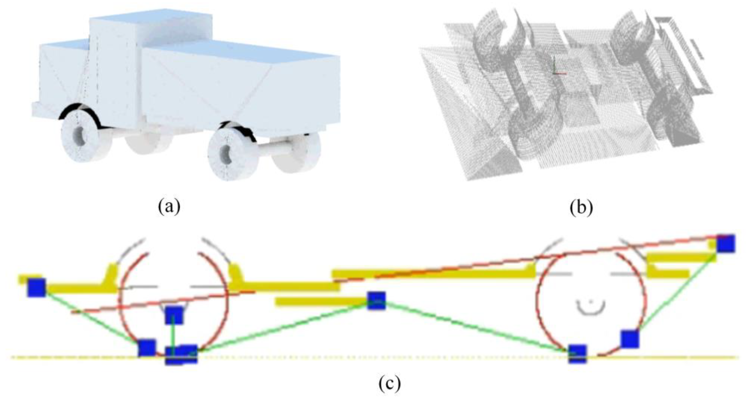
The experiment was conducted in a parking lot, and the hardware system used in the experiment is shown in Figure 7.

Figure 1 shows the experimental process, where a wheeled robot is programmed to move underneath the stationary vehicle at a constant speed. During this motion, the robot acquires and builds point clouds, enabling the calculation of the passing angles.

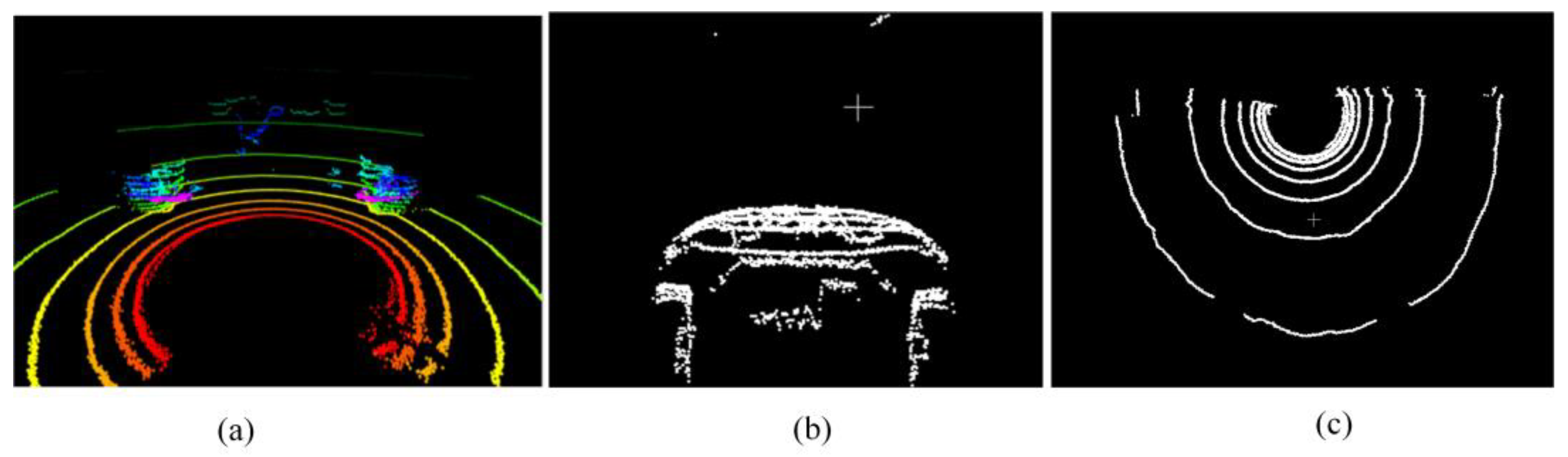
The first step in the experiment is the selection of segmentation methods. We conducted experiments using frames from the LIADR to evaluate the effectiveness of segmentation using sphere and plane models to determine suitable models and coefficients.

As shown in Figure 8a,b, the segmentation results demonstrate that both circular and planar shapes can successfully segment ground point clouds. In Figure 8, it can be observed that the outermost laser line in Figure 8a appears to be more complete compared to Figure 8b. Furthermore, the segmentation results are also influenced by the choice of coefficients. Figure 8c,d show the results of over-segmentation, where points belonging to the vehicle are influenced as ground points due to the selection of inappropriate coefficients.

To minimize the proportion of ground points without over-segmentation, we extracted frames from five regions of the vehicle for analysis. These five regions are located at the front wheels, the rear wheels and the front, middle and rear of the vehicle. Analyzing the frames selected from these five regions can provide a more generalized representation of the vehicle. Here, we segmented these frames using different segmentation coefficients and models, and the segmentation process was repeated five times. The results were then averaged and are shown in Figure 9 and Figure 10.

The relationship between the number of points and the segmentation coefficient is shown in Figure 9. Based on objective evaluation, we observed that although there are differences in the distribution of ground points segmented by plane and sphere models, shown in Figure 8a,b, the number of ground points is actually similar.

The time consumption of the segmentation performed using the plane and sphere models is shown in Figure 10. We can see that the segmentation using the plane model has the lowest cost and provides a stable performance.

Over-segmentation causes the point clouds of vehicle tires to be incorrectly segmented as ground point clouds. However, these over-segmented ground point clouds have a much wider distribution on this normal. Therefore, we calculated the over-segmentation threshold coefficients based on the distribution of ground point clouds on the normal. We performed statistical analysis of the distribution of the ground point cloud on its normal to determine whether the coefficients lead to over-segmentation. This was confirmed using the method of subjective evaluation, as shown in Figure 8c,d. The point clouds of the vehicle tires appear higher on this normal. Therefore, we automatically determined the over-segmentation threshold coefficients based on the distribution of ground point clouds on the normal. Based on the results shown in Figure 8, Figure 9 and Figure 10, we selected the plane model with a coefficient of 0.03 for segmentation. Additionally, Figure 11 shows the segmentation performance of an actual acquisition, where the ground and vehicle points are clearly segmented, effectively reducing the proportion of ground points.

We acquired the data underneath the vehicle using our system and compared the existing mature methods of point cloud building with our method. As shown in Figure 12, we found that the point cloud built by the ICP registration tool in PCL [20,31] (Point Cloud Library) exhibited an obvious alignment error in Figure 12a, and the method [22] failed to build a point cloud, as shown in Figure 12b, making it difficult to identify. The red square represents odometry data, which further confirms the failure as the wheeled robot is moving straight during the acquisition. Figure 12c,d show different views of the point cloud created by the method in [21], demonstrating distortion. On the other hand, Figure 12e,f show a better alignment result and an overall point cloud with improved geometric quality obtained using our method for parameter calculation. This is attributed to the close proximity of the wheeled robot to the ground during the acquisition of point cloud data from the underside of the vehicle, resulting in a small area of interest on the vehicle and a limited number of points. The introduction of a significant amount of error occurs during the ICP calculation process, and the circular shape of the ground points tends to lead to local optima during frame matching, particularly in the roll direction. Additionally, the scarcity of points on the vehicle, especially in terms of corner features, combined with the participation of numerous plane features from the ground points in the matching calculation, makes the matching process difficult to converge and even results in complete failure.

The effectiveness of the odometry module in building point clouds in our method is evaluated and compared with the laser odometry. As shown in Figure 13a, the laser lines in the marked area exhibit a significant tilt when the point cloud is created using the laser odometry. Conversely, the point cloud using the odometry reduces the tilted laser lines in Figure 13b, indicating its advantage in enhancing the constraint in the pitch direction and reducing error. This improvement is attributed to the matching process in visual odometry, where the feature points are mainly concentrated in the region of the vehicle, providing stronger constraints in the pitch direction.

Figure 14 shows the comparison of ground segmentation and the removal of outlier points in our method. In Figure 14a, the presence of floating shadows is caused by misalignment, while the jagged edges of the tires result from outliers and other interference points when directly aligning with laser feature points. Figure 14b,c show the point cloud results after solely removing ground points or outliers, respectively. It can be observed that only removing ground points or outliers leads to alignment errors in different directions and degrees. Figure 14d shows the overall point cloud in our method after reducing the proportion of ground points and removing outliers. This results in the effective reduction of floating shadows and jagged edges, thereby facilitating further processing of the point cloud.

To verify the calculation method of the angles proposed in our study, we utilized a simulation vehicle model created in AutoCAD. The design of the module used for calculation is shown in Figure 15, and the results of the 10-time calculation for the simulation model are presented in

Table 1. Calculation results of the simulation model.

Parameters	True Value	Calculated Value	Error
Approach	28.79°	28.772°	−0.06252%
Departure	44.44°	44.433°	−0.01575%
Ramp Breakover	30.10°	30.1012°	0.003987%

.

The results of the passing angles are shown in Table 1. We captured the point cloud of the vehicle’s underside using a perspective view of the wheeled robot and calculated the angles using our proposed method. Since the truth-value of the vehicle is easily obtained in the simulation, we directly compared the calculated results with the simulated truth. The consistency of the calculated results was confirmed by performing 10 runs, with only negligible errors observed.

Additionally, we performed the experiments three times on a real vehicle and calculated the passing angles ten times in each experiment. The results of passing angles are shown in

Table 2. Statistics of the calculation results.

Angle	Approach	Departure	Ramp Breakover	Variance
Experiment 1	47.6402° (10)	44.0219° (10)	34.7180° (10)	0
Experiment 2	46.9971° (10)	44.9910° (10)	32.6791° (10)	0
Experiment 3	46.8205° (10)	45.7268° (10)	33.8514° (10)	0
Average	47.1526°	44.91323°	33.7495°	-
Variance	0.12407	0.48747	0.69804	-

.

In actual engineering measurements, deviations in points selection and measurement often lead to significant discrepancies in the results obtained by different personnel, making it challenging to obtain accurate and reliable values. Our results demonstrate that the robustness of our system can mitigate measurement errors, with angular deviations during repeated experiments being less than 1°, satisfying the requirements of measurement.

5. Discussion

The automated measurement of the passing angles of vehicles has been developed slowly due to environmental constraints, making it challenging to address disputes encountered in actual engineering measurement. In this paper, we introduced a wheeled robot equipped with a LIDAR and a camera into the measuring process, taking into account various interference factors in data collection and calculation. Our system has been successfully deployed and has played a role in data comparison during enterprise bidding processes.

In this study, the results of the overall point cloud have proven the effectiveness of the method, as they exhibit few errors and little drift, as shown in Figure 12, Figure 14 and Figure 15. This is achieved by reducing the proportion of ground points that do not contribute to frame matching, avoiding the selection of unstable feature points during the feature extraction process and smoothing the odometry. These measures effectively reduce matching errors, inaccuracies and significant drift. We conducted simulation experiments to verify the accuracy of the computational method and performed field experiments to validate the feasibility and robustness of the proposed method and system. The calculated passing angles in simulation had a norm error of 0.06252% for the approach angle, 0.01575% for the departure angle and 0.003987% for the ramp breakover angle compared to the true value. Additionally, we conducted three groups of experiments using the system, each consisting of ten repetitions of the calculation, resulting in variances of 0.12407 in the approach angle, 0.48747 in the departure angle and 0.69804 in the ramp breakover angle. Based on the simulated and experimental results, the method and system were validated.

The measurement system and method proposed in this paper enable the efficient acquisition of the point cloud of a vehicle body and compute the passing angles with high data consistency. This system, coupled with the proposed method, reduces manual labor, improves measurement efficiency and mitigates data controversy caused by manual experience-based selection of target points for measurement. Moreover, the method proposed in this paper also brings reference to the intelligent measurement of geometric parameters for various kinds of large equipment.

6. Conclusions

This paper presents a measurement method and system for the automatic, efficient and robust measurement of vehicle passing angles.

The proposed measurement method consists of two parts: the point cloud building and the parameter calculation. The point cloud building system utilizes a remotely operated wheeled robot to construct a high-quality overall point cloud underneath the vehicle. The parameter calculation part accurately and robustly measures the passing angles from the point cloud without relying on manual experience. The experimental results demonstrate the validity of the proposed method and system. However, the inherent noise of the LiDAR sensor has not been completely eliminated, which imposes a limitation on improving measurement accuracy. In the future, our work will integrate standard references to optimize the overall point cloud, enhancing its ability to reflect the real geometric information of objects and improving overall data accuracy. Additionally, we will expand our research to include multiple vehicle types to validate its wide applicability.