Abstract
During the interception of a high-speed gliding vehicle (HGV), the predicted intercept point (PIP) is updated many times, so the interceptor must continuously adjust its trajectory. In this paper, we propose an online guidance correction algorithm for the interceptor, which can effectively meet the position constraints and energy management of the guidance process. Firstly, we simplify the interceptor’s maneuvering problem to a two-body orbital transfer problem. The Lambert orbit transfer method is used to enable the interceptor to maneuver towards the target’s PIP. Secondly, by comparing the target’s high probability existence area (THPEA) with the interceptor-interceptable area (IIA), the engine start threshold is set in stages to avoid frequent redundancy maneuvers caused by frequent engine starting during missile correction. This approach achieves energy management. Simulation results show that our midcourse guidance strategy is effective.
1. Introduction
With their high speed, high maneuverability, and a large airspace, high-speed gliding vehicles (HGVs) pose significant challenges for defense systems. Multi-stage guidance for the interceptor is an effective method, and the entire flight of the interceptor can be divided into three stages: the boost stage, the midcourse guidance stage, and the terminal guidance stage. The main role of the boost stage is to make the interceptor lift off quickly. The midcourse guidance stage guides the interceptor to the vicinity of the HGV based on limited target information. Once the target seeker turns on and discovers the HGV after meeting the position constraint, the interceptor enters the handover of midcourse and terminal guidance, and the terminal guidance stage uses the information obtained by the target seeker to achieve the final intercept. The midcourse guidance plays an important role in determining whether the interceptor can successfully enter the terminal guidance stage to capture the target.
The method based on the predicted intercept point (PIP) is a common approach in midcourse guidance for guiding the interceptor to the vicinity of PIP [1,2]. However, factors such as the detection accuracy, prediction accuracy of the target trajectory, and target avoidance maneuver may prevent the defense system from determining the final PIP at one time. There will be more than one continuously updated PIP during the interceptor’s flight, and the interceptor has to make trajectory corrections according to the updated PIPs. As shown in Figure 1, the interceptor corrects the trajectory twice in the midcourse guidance stage due to two PIP updates. When the PIP is updated for the third time, the interceptor flies near the target and enters the terminal guidance stage. This figure is only a schematic diagram, and the actual process will have more than three PIP updates.
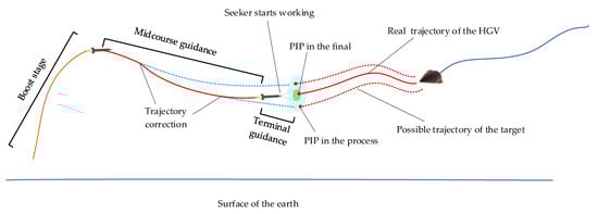
Figure 1.
Interceptor and target location diagram. The trajectory of the interceptor can be divided into the boost stage, midcourse guidance stage, and terminal guidance stage. The target trajectory is uncertain, resulting in the continuous updating of the PIP. The function of the midcourse guidance stage is to guide the interceptor to the vicinity of the final PIP, which facilitates the target acquisition by the seeker in the terminal guidance phase.
When the trajectory prediction is more accurate, the defense system can obtain more precise PIP location information. Although some researchers have studied the problem of predicting target trajectories [3,4,5], no study has been able to accurately predict a target’s trajectory. With the arrival of HGVs, the amount of target information and trajectory prediction accuracy increases, leading to discrete updates of PIP during the flight of the interceptor in midcourse guidance. The PIP at one moment may differ significantly from the next, making continual corrections necessary until the terminal seeker captures the target. Based on this analysis, the two main difficulties of the problem are:
- (1)
- Uncertainty in PIP updates during midcourse guidance. To overcome the uncertainty and reach, the true PIP vicinity at the end of the midcourse, the interceptor must continually modify its trajectory with online correction strategies.
- (2)
- The need to conserve energy during midcourse guidance by avoiding unnecessary maneuvers. Direct force maneuvering would still require fuel in the terminal guidance stage.
Therefore, the key is to formulate an online correction strategy for the interceptor when PIP is randomly updated, ensuring that the interceptor reaches the terminal guidance with a certain level of accuracy while saving fuel and leaving a sufficient maneuvering margin in the terminal guidance stage.
When the trajectory tracking error is large or the target maneuvers, the interceptor needs to correct the existing flight trajectory. There are two types of correction algorithms applied to the trajectory correction problem. The first type is to re-optimize a trajectory for the interceptor, and some researchers propose the method of the online re-optimization trajectory according to the changes of state and constraint. In [6], an improved zero effort miss and zero effort velocity (ZEM/ZEV) guidance law was proposed for the guidance of anti-ballistic missiles outside the atmosphere. According to the updated terminal conditions, a flight trajectory was re-optimized. Some experts also used the polynomial function [7], multiple shooting method [8], and particle swarm optimization method [9]. In [10], an online trajectory planning algorithm was proposed to meet the current and terminal constraints, and then a simple guidance law was used to track the reference path. Some experts have also used convex optimization to generate trajectories online by virtue of its high efficiency for low thrust re-entry trajectory planning, landing path planning, and orbital transfer [11,12]. In [11], an online guidance framework based on convex programming was proposed, and a command correction method was designed to reduce the delay effect based on the sensitivity analysis of nonlinear programming. Reference [13] proposed an autonomous entry guidance algorithm based on the convex programming theory, which could plan a new trajectory online. To improve the efficiency of online solutions, some researchers also proposed combining different methods. For example, references [14,15] referred to the combination of the model predictive control (MPC) method and convex optimization. Based on the model predictive static programming, reference [16] established a new convex programming framework to solve the optimization problem in a computationally efficient way. Reference [17] proposed an improved continuous convex algorithm based on pseudo-spectrum to solve the rocket landing problem, which has high accuracy and computational efficiency by combining the pseudo-spectrum discretization and convex optimization. Although these methods made efforts to improve the computational efficiency constantly, multiple optimizations were inevitably needed in the multiple-update process of the PIP, which would bring a significant burden to the airborne calculation and affect the computational efficiency.
Other methods are unwilling to abandon the nominal trajectory, as they prefer generating a suboptimal trajectory or developing online guidance instructions based on the original nominal trajectory according to the change of terminal constraints, rather than re-searching the appropriate correction instructions in a large allowable domain to carry out online correction as in traditional research. If the modified terminal constraint or disturbed state is not far from the original constraint or disturbed state, the original nominal trajectory can be used to generate a new trajectory through the adjacent optimal control theory. In [18,19,20], the terminal position modification was allowed by taking the current state disturbance and the modified terminal constraint as the feedback input, and the control modification was generated by further distinguishing the first-order optimality conditions, all of them used the indirect Legendre Pseudospectral feedback method to design a robust state feedback guidance law to offset the initial trajectory perturbation. In [21], an online optimal midcourse trajectory correction algorithm was designed to make full use of the nominal trajectory information by solving the terminal second-order equation and integrating the disturbance dynamics equation back to the initial time, so the problem of the co-state disturbance being difficult to express was solved. A new online guidance method based on the predictive guidance algorithm and neural network theory was proposed in reference [22], which could guarantee the guidance accuracy in real-time guidance. Based on the neighboring optimal control theory, reference [23] proposed a general guidance method to obtain the integrated guidance and control instructions online. The above methods avoid repeatedly reoptimizing the trajectory, so they achieved a high solving efficiency. However, due to the optimization near the nominal trajectory, it cannot cope with the situation that the terminal constraint update range is large and the updated law is uncertain. Some references attempted to introduce the rolling time domain control method [24], the model predictive static programming method [25], and the iterative guidance method [26,27] to continuously and iteratively correct the trajectory, but they could not effectively solve the problem of the PIP random update in a wide range.
Combining the above two types of correction algorithms, we can see that reoptimizing the trajectory method requires a large amount of computation, because the target’s PIP will be updated multiple times during the interceptor’s guidance process, and the exact coordinates of the next update are unknown; as such, using this method will significantly increase the computation of the computer, and while the second method of correction based on the nominal trajectory is less computationally intensive, it is only applicable to the PIPs updated in a small range. Neither correction method can be applied to the actual situation where the target PIPs are updated in a wide range.
In addition, fuel savings in the midcourse guidance need to be considered to ensure that the interceptor has sufficient maneuvering capability in the terminal guidance. To solve the fuel-saving problem of spacecraft in orbit correction and realize energy management, the study in [28] introduced piecewise linear and exponential damping, changing the sensitivity of target maneuvering with the distance between the missile and the target; however, it was mainly aimed at the terminal guidance stage with clear target information, which could not be suitable for the midcourse guidance with uncertain target position information. For the space rendez-vous problem of spacecraft and non-cooperative targets, the differential game was used to describe the pursuit–evasion game problem under continuous thrust in reference [29]. The optimal control and game theory were combined to achieve the optimization of fuel consumption in the process of intercepting non-cooperative targets. However, as the basis for solving this problem, the motion model of non-cooperative targets was clear. In reference [30], an analytical calculation method based on vector form was proposed for the Lambert dual-pulse rendez-vous problem with optimal energy and optimal fuel, and the vector form analytical solution of the Lambert dual-pulse rendez-vous problem with optimal energy and optimal fuel was given, which effectively improved the fuel consumption.
The motion models of the targets in the above studies are clear, but in this paper, the target’s maneuvering model is unknown, the update law of the PIP is random, the target is active in a discrete and dynamic spatial environment, the prior knowledge is incomplete, and the subsequent information is not clear. Furthermore, to achieve online real-time trajectory correction, then not only must the computer efficiency and correction accuracy be balanced, but the fuel-saving ability of the interceptor must be ensured.
In this paper, we propose a midcourse guidance method for guiding the interceptor to the final PIP while reducing fuel consumption. The method takes the HGV as the interceptor target and utilizes the target high probability existence area (THPEA) model to describe the gradual convergence process of the PIP error range, which provides terminal position constraints for midcourse guidance. We adopted the Lambert orbit correction method based on the two-body theory for midcourse guidance and designed an engine start-up threshold changing strategy to avoid unnecessary start-ups while meeting the terminal position constraint with low fuel consumption. The main contributions of this study are as follows:
- (1)
- We establish a two-body motion model of the interceptor that simplifies subsequent calculations by ignoring the weak influence of aerodynamic force. We also established the THPEA model of the target and describe the PIP point update law of the interception process, which provides terminal constraints for midcourse guidance.
- (2)
- For a single PIP, we achieve interceptor correction through velocity gain guidance based on Lambert’s variable trajectory theory. This method is more suitable for scenarios with a wide range of terminal position constraints than existing correction methods.
- (3)
- For continuously updated multiple PIPs, we introduce a method of setting the engine start-up threshold in stages based on the correction of a single PIP. This ensures that the interceptor meets the terminal constraints and avoids redundant maneuvering.
The rest of this study is organized as follows. Section 2 introduces the motion model of the interceptor. Section 3 introduces the online dynamic correction strategy for the interceptor we designed, which mainly includes the online correction strategy for the single PIP and the strategy for the multiple PIP update. In Section 4, numerical calculations and comparative analyses were performed. In Section 5, our conclusions, contributions, and innovations are explained.
2. Model Description
2.1. Introduction of Coordinate System
- (1)
- East–North–Up coordinate system
The East–North–Up coordinate system takes a local observation point as the origin, with the northward direction, eastward direction, and upward direction as its coordinate axes. It can accurately describe the three-dimensional spatial coordinates of a geographic location. Using the East–North–Up coordinate system, one can determine the distance, angle, and orientation between the current location and the target location, which enables navigation and positioning functions.
- (2)
- Geocentric coordinate system
The geocentric coordinate system is a spatial Cartesian coordinate system constructed with the Earth’s center as the origin, the unit vector direction from the Earth’s center to a specific location as the Z axis, and a reference plane as the X–Y plane. The geocentric coordinate system can be used for celestial dynamics calculations. By calculating the motion trajectory, velocity, acceleration, and the other parameters of celestial bodies in the geocentric coordinate system, the future paths of celestial bodies can be predicted.
2.2. Motion Model of the Interceptor in Midcourse Guidance
An interceptor with multi-stage vectored thrust engines is investigated in this paper. The whole process of interceptor flight can be divided into the boost stage, midcourse guidance and terminal guidance. The boost engine works in the boost section, and the vectored thrust engine works to provide a maneuvering capability during midcourse and terminal guidance. The difference between the midcourse and terminal is whether the target seeker is on or off, and the target seeker only works in the terminal guidance. Therefore, the task of the midcourse guidance is to guide the interceptor to the vicinity of the target. The interceptor in the midcourse guidance and the terminal guidance are mainly driven by the engine system. The thrust direction is along the axis direction of the interceptor and passes through the interceptor centroid. By adjusting the attitude of the interceptor, the interceptor can maneuver in different directions. The attitude of the interceptor is determined by six attitude control engines distributed around the interceptor. The configuration of interceptor is shown in Figure 2. Due to the small distance covered by the interceptor compared to the Earth’s circumference, and because the fuel consumption for most regular missiles is often assumed to be a constant value in calculations, the two following assumptions are made:
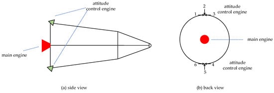
Figure 2.
Interceptor configuration. The attitude of the interceptor can be controlled by six attitude control engine combination switchers for three channels, of which engines No. 2 and No. 5 can be used for pitch channel control; (No. 1 + 6) and (No. 3 + 4) can be used for yaw channel control; and (No. 1 + 4) and (No. 3 + 6) can be used for roll channel control.
- (1)
- The engine exhaust velocity and the normalized mass burn rate are constants;
- (2)
- A nonrotating sphere model without J2 perturbation is used to describe the relationship between the state parameters and other variables.
In the East–North–Up coordinate system, the motion model of the interceptor in midcourse guidance is
where represent the positional coordinates in the East–North–Up coordinate system; denote the individual components of the velocity vector; is the mass of the interceptor; is the initial mass; is the thrust of the engine; represents the engine on–off instruction; and are the pitch angle and yaw angle; are the resistance, lift, and lateral force; are the inclination angle, trajectory deviation angle, and trajectory inclination angle; represent the components of the gravitational acceleration under the central gravity field in the East–North–Up coordinate system; and is the fuel consumption per second of the engine.
where the sea-level atmospheric density , is the reference height.
It pointed out in [31], for an interceptor flying with a high throw reentry trajectory and a height above 80 km in midcourse guidance, the magnitude of the aerodynamic force that can be utilized is negligible, and the ballistic correction capability is primarily limited by the energy that can be used by the orbital control engine. Therefore, the aerodynamic force could be ignored, and Equation (1) can be simplified as
2.3. Motion Model of Interceptor in Geocentric Coordinate System
Considering the fact that the interceptor is slightly affected by aerodynamic force in the midcourse guidance stage, the maneuvering process of the interceptor in the midcourse guidance can be regarded as the orbit transfer process in the geocentric coordinate system in this paper, and the motion model is
where is the Earth center vector, is the velocity vector of the interceptor, and is the thrust direction of the engine. The gravity acceleration of the interceptor is
it can be seen from Equation (4) that the simplified interceptor motion model is equivalent to the two-body motion model. Therefore, in the case of weak aerodynamic force, the moving process can be regarded as two-body motion, and the trajectory characteristics of the interceptor with direct force adjustment are consistent with the two-body trajectory characteristics.
In geocentric coordinate systems, the position vector and velocity vector of the interceptor at the instant are known, and it can be obtained that
the position and velocity vector in (6) determine the characteristic root number of the interceptor, where is the semi-major axis of the hyperbolic trajectory, is the eccentricity, is the inclination angle of the trajectory, is the longitude of the ascending point, is the amplitude angle of the near-day point, and is the angle of the epoch approaching point. The specific solving process is shown in reference [32] Conversely, according to the law of orbital transfer, if the number of orbital elements of the interceptor orbit is known in the orbital maneuver, the orbital characteristics at all positions in the orbit can be obtained by adding time. Namely
after establishing the motion model of the above two coordinate systems, each variable can be expressed through the conversion between the two coordinate systems.
2.4. Calculation of Required Velocity Based on Lambert Guidance
With the required velocity, the interceptor can reach the target in a certain terminal constraint according to the current state of inertial motion without any additional orbital maneuver. Therefore, the first step is to solve the required velocity of the interceptor. Most interception tasks require the interceptor to reach the target PIP at a fixed time, as arriving too early or too late will result in a failed interception. Solving the required velocity in the interceptor’s trajectory transformation is the classical Lambert problem, which belongs to solving the two-point boundary value problem under the two-body theory.
The essence is to solve the speed problem of fixed time flight. As shown in Figure 3, the spacecraft is required to fly from point to point , where point represents the Earth’s center and is the transfer angle. At the initial time, the spacecraft is at point and the velocity is ; if not adjusted, the interceptor will fly to the point after time . When the velocity is at point , the spacecraft will fly to the target point after time . The solution of is the problem solved by Lambert.
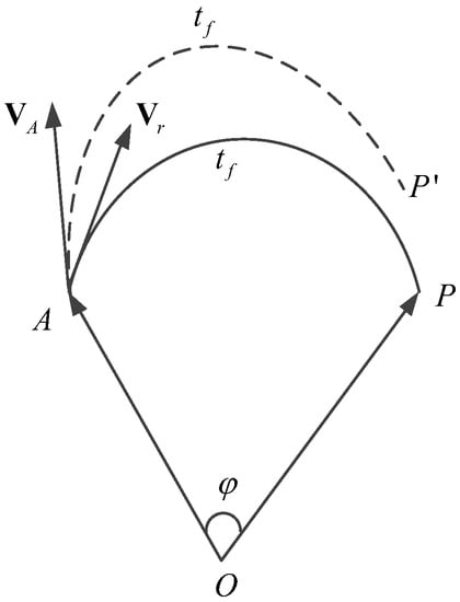
Figure 3.
Required velocity diagram.
Referring to the required velocity solution for a ballistic missile in-flight, when given the initial track angle and required distance, the missile’s initial speed must be sufficient to hit the target on the ground.
where
is the initial height of the missile relative to the surface. Extend the speed equation
where is
where refers to the height of the target.
Under elliptical trajectory, the time required for missile and target encounter is
where is the speed required to intercept the target and represents the energy parameter. The transfer angle can be obtained when the initial position vector and the end position vector are known in the geocentric coordinate system. is the flight transfer angle, which can be expressed as
According to Equation (10), Equation (12), and Equation (14), we can obtain
where is the required speed of trajectory transformation. Since the required speed cannot be directly obtained, the trajectory angle iteration method can be used to quickly solve the required speed in the Lambert problem, and the solution process is detailed in reference [33].
3. Design of Online Dynamic Correction Strategy for Interceptor
3.1. The Description of THPEA
In the actual interception process, the longer the defender tracks, the more trajectory information is obtained, and the accuracy of the trajectory prediction improves accordingly. This indicates that the PIP is constantly updated. In this paper, we refer to all areas where PIP may occur as targeting high probability existence areas (THPEA). As the warning detection system becomes more accurate, the THPEA will continue to reduce, which is consistent with an increase in target detection information.
The calculation of the PIP position coordinates requires the estimation of target measurement information, target state continuous tracking, and prediction. If the instant of midcourse and terminal guidance trajectory transition is , the instant of the early warning system that starts to track the target is , then the total flight time satisfied . The target trajectory tracking refers to the extraction of the target measurement information with noise between the initial tracking instant and the current instant by the early warning detection system, and the duration is . According to the extracted target state information, different model sets are selected, and the model set and interactive multi-model algorithm are used to track the real trajectory of the target. Then, the future flight trajectory of the target is predicted based on the current state estimation and the model probability of each model set. The prediction stage starts from the current instant and finishes at the transition instant , which indicates that the interceptor needs to predict the flight trajectory of the target in the future time , and the target prediction trajectory is extrapolated to determine the PIP and the THPEA. Since there is no measurement information of the target during the period , the prediction of the target trajectory at the future time will show a divergent trend: the longer the prediction time is, the larger the error is. The work in each stage and the work timing relationship are shown in Figure 4.
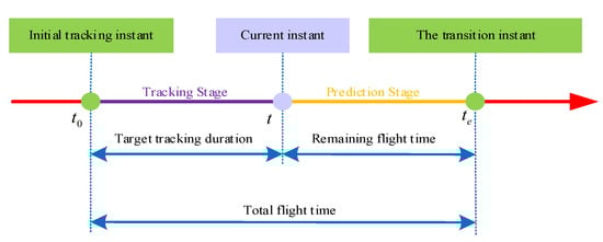
Figure 4.
Time-series relationships for target trajectory prediction. In the tracking stage, the measurement information of the target can be obtained, and the trajectory prediction is to predict the trajectory of the target in the prediction stage by the measurement information in the tracking stage.
The mathematical expectation of the target position coordinates under the axes is , and the variance is . The three-position coordinates of the target are independent from each other. In reference [32], the coordinates obey Gaussian distribution, and the probability density function of the target position at a certain time is
among them
therefore, when the target tracking state converges, according to the rule, the probability of the target position distributed in is 0.6827, the probability distributed in is 0.9545, and the probability distributed in is 0.9973. It can be considered that the target position is almost entirely concentrated in the three ellipsoid regions with the mathematical expectation coordinate as the center and the axial direction of . Therefore, the target THPEA (region) is defined as follows:
Definition 1.
The THPEA is an ellipsoid area with a trajectory expectation as the center and thevariance of the independent distribution of the target position as a three axial radius. As shown in Figure 5.
Figure 5.
The dynamic change process of the PIP and THPEA of high-speed gliding target.
The area size is related to the variance of the target coordinate distribution. After the interceptor is launched, the early warning detection system improves its target tracking accuracy over time. As a result, the distribution variance of the target’s position will inevitably decrease. The change in is related to time, at the next instant, ,
as time goes on, the variance of the target position distribution tends towards , and the THPEA of the target will gradually converge towards the real PIP. Figure 5 shows the change process of the THPEA.
It can be seen from the above analysis that the dynamic updating of the THPEA is mainly reflected in the variances , and of the target position distribution on the , , and axes. In practice, the variance of the target’s position distribution is related to the target maneuvering mode, trajectory prediction algorithm, and other factors, and its change rule is only applicable for specific targets.
3.2. Modeling of the Interceptor-Interceptable Area
The interceptor-interceptable area (IIA) is the maximum maneuverable range of interceptors in the terminal guidance stage. When the starting time of the interceptor seeker is , the maximum working time of the terminal guidance is , the steady thrust of the engine is , the specific impulse is , and the mass of the interceptor missile at the starting time of the seeker is , so the mass change rate is
at a certain instant in the terminal guidance stage, the lateral maneuvering acceleration of the interceptor is
if the interceptor maneuvers with the maximum maneuvering acceleration, the lateral speed and the maximum lateral maneuvering displacement of the interceptor at instant are
the interception instant is denoted as . If , the maximum lateral displacement of the interceptor perpendicular to the direction of the initial velocity vector is
if , the maximum lateral displacement perpendicular to the initial velocity vector is
therefore, the IIA of the interceptor can be expressed as
where are the coordinates of the PIP point in the East–North–Up coordinate system. The IIA is shown in Figure 6.
Figure 6.
The IIA of interceptor.
3.3. Design of Online Correction Strategy for Single PIP
For a single PIP, according to the interceptor position vector , flight velocity vector , and remaining flight time , the required velocity and engine thrust direction could be solved. By determining the interceptor’s engine switch logic in the midcourse guidance stage, the interceptor engine can be timely switched on for online correction. An online correction algorithm for the interceptor in the midcourse guidance is designed as shown in Figure 7.
Figure 7.
Design of midcourse guidance correction algorithm based on velocity gain guidance.
The specific description is as follows:
Step 1: After the target is detected by the early warning detection system, the defense system calculates the PIP (PIP in Figure 1) and launches the interceptor;
Step 2: According to the position and velocity in the East–North–Up coordinate system of the interceptor, through coordinate system transformation, the velocity vector and position vector of interceptor under the geocentric coordinate system are obtained, the remaining flight time given by the interceptor mission and the position vector of the PIP, the required velocity could be solved by the method in Section 2.3. Then, the velocity gain could be obtained, where
Step 3: To save fuel, there is no need for the continuous start-up of the engine, a certain start-up threshold should be set, and is the engine start-up threshold in this paper. If , start the engine, and the starting direction is
the time of the engine starting is recorded, and the position and velocity information after one step of maneuver is solved integrally. Continue with step 2. To avoid system instability caused by a too short engine start-up time, set the shortest engine start-up time , if and shut the engine down and clear recorded starting instant ; if , then, keep the engine on.
Step 4: Continue the above process until .
3.4. Design of Online Correction Strategy for Multiple PIP Updates
The main focus of this section is on the switch between engine start-up thresholds based on IIA and THPEA.
During the process of the interceptor flight, unpredictability in PIP updates means that the speed gain is not zero for a long time after each update. At this point, if the engine start threshold is set to the ideal condition , then the frequently adjusting engine needs to stay operational throughout the midcourse guidance stage, resulting in excessive fuel consumption, which would diminish the intercepting capabilities at the final guidance stage. Therefore, it is imperative to set the starting threshold for the engine to prevent such waste.
Since the PIP appears randomly, it is difficult to determine whether the PIP maneuver at the current instant is redundant. It can be seen that, in the initial stage, the variance of the target position prediction distribution and the THPEA is large. Over time, the tracking time for the target increases, the remaining time of trajectory prediction becomes shorter, and the accuracy of the target trajectory prediction increases. The THPEA gradually converges, which means that the closer it is to the end of midcourse guidance instant, the smaller the THPEA. At the stage of a large THPEA, the interceptor needs to respond to the update of PIP and correct the trajectory through the engine opening in time. As the interceptor flies, the THPEA will continue to converge, the update range of PIP will be reduced, and the maneuvering requirement for the interceptor will be weakened. At a given time, the interceptor could achieve the IIA coverage of THPEA, which means that even if the PIP still updates randomly, it is still within the IIA range of the interceptor and the interceptor no longer needs to perform additional maneuvers.
The cover instant of the IIA to the THPEA is regarded as the stage switching point. By setting the start-up threshold in stages, the interceptor can complete the large deviation correction before the stage switching point, and avoid the frequent start-up in the later stage, which can reach the final PIP based on effective fuel saving.
According to the analysis of the THPEA in Section 3.1 and Section 3.2, the variance change rule of the target location prediction is obtained. The variance of the target position prediction at instant is , , and . According to the criterion, the radius of the ellipsoid formed by the THPEA on three axes is
since the distribution of target PIPs on the three-coordinate axes is independent for each one, has the greatest impact on the distribution of target PIPs.
According to Equation (32), the range of the IIA satisfies , and is the maximum lateral displacement. In the interception process, if , it indicates that the maximum IIA cannot cover the THPEA at the current instant, and that large-scale maneuvering correction is still needed; if , it means that, at maximum, the IIA can cover the THPEA. Even if there is a certain deviation in the midcourse guidance stage, the target can be successfully intercepted by the terminal guidance maneuver after the seeker starts. There is
where is the engine start threshold in the first half stage and is taken to ensure the correction capability of the interceptor in this stage; is the starting threshold of the engine in the later stage. To ensure the correction ability of the interceptor in this stage, the value of is slightly larger, depending on the allowable miss distance. The larger the acceptable miss distance is, the larger the value of is.
Figure 8 shows the main work content of this paper. The primary work is divided into two parts: Section 3.3 mainly addresses the issue of ensuring that the missile accurately reaches the final true PIP, while Section 3.4 aims to prevent frequent engine start-up and optimize the fuel consumption as much as possible in the context of PIP up-dates.
Figure 8.
The diagram illustrates the work content of this paper. The main objective of this paper is to correct the interceptor during the midcourse guidance stage, in order to more effectively cope with constantly updated PIPs while saving fuel as much as possible. The primary work is divided into two parts: Section 3.3 mainly addresses the issue of ensuring that the missile accurately reaches the final true PIP, while Section 3.4 aims to prevent frequent engine start-up and optimize the fuel consumption as much as possible in the context of PIP updates.
4. Simulation Verification
This section mainly conducts simulation verification on the proposed algorithms. The simulation software we used is MATLAB R2014a, and the computer processor used for simulation is intel(r) core(tm) i7-10700cpu @ 2.90GHZ with an installed memory of 8.00GB.
4.1. Simulation Scenario 1: Online Correction Algorithm for Single PIP
The position coordinate of the PIP in the East–North–Up coordinate system is , the initial position coordinate of the mid-course guidance is , the remaining flight time of the interceptor is , the initial speed of the interceptor is , and the thrust of the orbit control engine on the interceptor is . The correction ability of the interceptor against a single PIP under the initial inclination angle deg is verified.
Figure 9 and Figure 10 demonstrate the changes in the interceptor’s maneuvering trajectory and speed guided by the velocity gain, respectively. It can be seen from Figure 9 that, under the guidance of velocity gain, the interceptor trajectory is smooth, which belongs to the high-drop reentry trajectory. Table 1 shows that the PIP can be reached with high accuracy under different initial trajectory inclination angles. At the same time, in Figure 10, the change in the magnitude of the velocity gain shows a convergence trend. There is a certain fluctuation between 70 s and 100 s in Figure 10. This is caused by the interceptor’s declining flight altitude and increased aerodynamic effects. Although some adjustments are necessary, they are minor. It is necessary to adjust the required velocity, but the adjustment is only a small amount. Therefore, it can be concluded that the guidance of velocity gain effectively resolves the aforementioned issue.
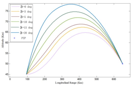
Figure 9.
Trajectory under different initial inclination angles.
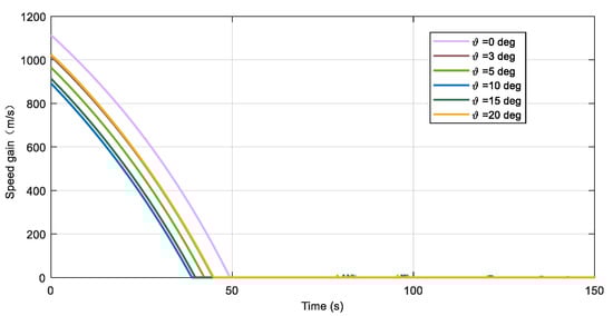
Figure 10.
Change in the speed gain under different initial inclination angles.

Table 1.
Guidance error and starting time under different initial inclination angles.
4.2. Simulation Scenario 2: The Online Correction Effect of the Designed Correction Algorithm for Multiple PIP Updates
Firstly, the staged threshold setting method is not adopted, and the starting threshold of the whole engine is . In the simulation, the update period of the PIP is set to 5 s, and a total of 30 updates occur in 150 s. The 3-fold variance of the PIP distribution at the initial instant is 10 km, which means . With the interceptor flying, the PIP converges to the real PIP in the error domain , and the initial inclination angle deg is verified.
It can be seen from Figure 11 that the trajectory of the interceptor conforms to the trajectory characteristics of high throw-reentry, and the blue points are PIPs for the update process, red points are the final PIPs. However, the interceptor still flies to the final PIP after correction. The overall correction trajectory is relatively smooth, and there is no large-scale trajectory change.
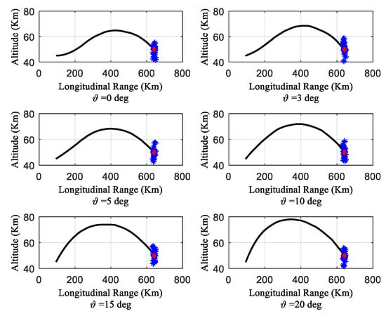
Figure 11.
Trajectory at different inclination angles for multiple PIP updates.
The final miss distance is 0.633 km, and the continuous start-up time of the engine is 62.28 s. It can be seen from Figure 11 and Figure 12 that the velocity gain guidance method can complete the midcourse guidance interception task. Due to the update of PIPs, the change process of the velocity gain in Figure 12 converges globally and fluctuates locally. The main reason is that the update of the PIPs leads to the change in the velocity gain, but it can eventually converge to a small value. Although the final accuracy is degraded, it can still meet the requirements of midcourse guidance, which shows that the online correction algorithm can satisfy the interceptor correction when the PIPs are updated multiple times.
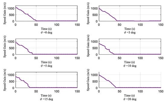
Figure 12.
Trend of speed gain at different inclination angles for multiple PIP updates.
4.3. Simulation Scenario 3: Verify the Effectiveness of Online Correction of Interceptor When Setting the Switch Threshold in Stages
Set a fixed threshold , to achieve the interceptor as far as possible not to start before stage the switching point, set the first phased threshold , and set the second phased . In the simulation, the update period of the PIP is 5 s. With the interceptor flying, the PIP finally converges to the real PIP . To verify the correction effect under the phase-setting threshold method and fixed threshold method when the 3-fold variance of the PIP distribution at the initial instant is , 20 Monte Carlo simulations are performed for each group.
Figure 13, Figure 14 and Figure 15 show the total engine start-up time, miss distance, and fuel consumption of the interceptor when the two methods conduct 20 Monte Carlo simulations, respectively. The initial conditions and the updated position coordinates of PIPs are identical for both methods.
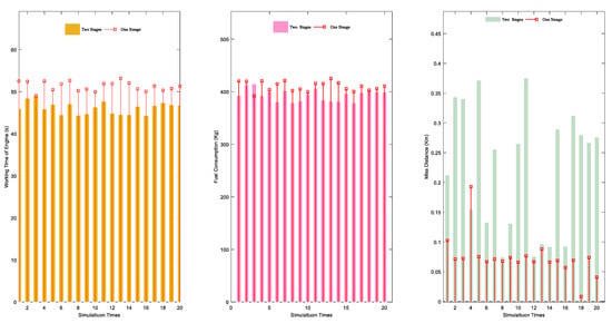
Figure 13.
Statistical results when the 3-fold variance of the PIPs’ distribution is 5 km.
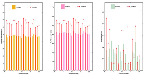
Figure 14.
Statistical results when the 3-fold variance of the PIPs’ distribution is 10 km.
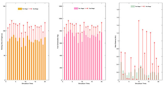
Figure 15.
Statistical results when the 3-fold variance of the PIPs’ distribution is 20 km.
In Figure 13, Figure 14 and Figure 15 two stages represent the method of the two-stage design of the engine start-up threshold, and one stage represents the method not used in the correction. It can be seen from Figure 13, Figure 14 and Figure 15 and Table 2 that, after the switching threshold is set in stages, the average start-up time and fuel consumption under the threshold set in stages are smaller than those under a fixed threshold. At the same time, the final average mass of the interceptor is greater than that with a fixed switch threshold. The miss distance by the two methods is equivalent, which both meet the requirements of midcourse guidance miss distance. At the same time, it can be seen that the three-fold variance in the PIPs’ distribution is larger, the range of the THPEA is wider, and the gap between the average start-up time, and the final average mass of the interceptor under the two methods is larger, indicating that the phased setting method has more obvious advantages for the interception scenario with wider THPEA.
Table 2.
The average of the results obtained under 20 simulations for each group of experiments.
5. Conclusions
An online correction strategy for a high-speed gliding target interceptor during midcourse guidance was designed in this paper. The Lambert guidance method was used to solve the engine starting direction, and the midcourse guidance correction strategy was designed. Furthermore, to avoid redundant maneuvering, the THPEA and its dynamic update law are analyzed. Based on the IIA covering THPEA, the threshold switching point is determined, and the switching threshold is set in stages to reduce the engine start-up time in the midcourse guidance phase. The simulation results show that the online correction algorithm proposed in this paper can guide the interceptor to meet the terminal guidance position constraints when the THPEA point is constantly updated. The proposed switching threshold method can effectively save fuel when the threshold of the first stage is and the threshold of the second stage is . Compared with the methods of regenerating optimal trajectories based on the target’s maneuver in documents [6,7,8,9,10,11,12,13,14,15,16,17], the method in this paper does not need to regenerate the optimal trajectory based on the updated PIP of the target, which avoids the huge computational cost brought by re-optimization. In addition, compared with the methods in documents [18,19,20,21,22,23,24,25,26,27], the correction algorithm in this paper is not limited to the original trajectory. If the trajectory needs to be changed, the engine start direction can be determined by the required speed, which is more suitable for the application scenario where PIP updates occur in a wide space and for intercepting high-speed gliding targets.
Although the correction method proposed in this paper can achieve rapid interceptor correction based on the randomly updated PIP during flight, thus achieving the purpose of fuel saving, this fuel-saving method is not the optimal solution, and the problem of fuel optimization requires further research. The next research direction for the authors will be how to develop an optimal fuel-saving correction method based on the constantly updated target PIP.
Author Contributions
Conceptualization, W.L., L.S. and T.Z.; methodology and other work, W.C. All authors have read and agreed to the published version of the manuscript.
Funding
This work was supported by the National Natural Science Foundation of China (Grant no. 62173339).
Data Availability Statement
All data generated or analyzed during this study are included in this published article.
Conflicts of Interest
The authors declare no conflict of interest.
Nomenclature
| Symbol | Meaning |
| HGV | High-speed gliding vehicle |
| PIP | Predicted intercept point |
| THPEA | Target’s high-probability existence area |
| IIA | Interceptor-interceptable area |
| The position coordinate in the East–North–Up coordinate system | |
| Velocity component in the East–North–Up coordinate system | |
| Mass of the interceptor | |
| Initial mass of the interceptor | |
| Engine on–off instruction | |
| Pitch angle of the interceptor | |
| Yaw angle of the interceptor | |
| Resistance, lift, and lateral force | |
| Inclination angle | |
| Trajectory deviation angle | |
| Trajectory inclination angle | |
| The component of the gravitational acceleration under the central gravity field in the East–North–Up coordinate system | |
| The fuel consumption per second of the engine | |
| Air density | |
| Center vector of the interceptor | |
| The velocity vector of the interceptor | |
| The thrust direction of the engine | |
| Gravity acceleration of the interceptor | |
| The semi-major axis of the hyperbolic trajectory | |
| Eccentricity | |
| Inclination angle of the trajectory | |
| The longitude of the ascending point | |
| The amplitude angle of the near-day point | |
| The angle of the epoch approaching point | |
| The transfer angle | |
| Required velocity | |
| Height of the target | |
| The energy parameter | |
| The midcourse and terminal guidance trajectory transition instant | |
| Total flight time | |
| Initial tracking instant | |
| The current instant | |
| The starting time of the interceptor | |
| The terminal guidance | |
| Specific impulse | |
| Interception time | |
| The mathematical expectation of the target position coordinates | |
| The variance of the target position coordinates | |
| Maximum lateral displacement perpendicular | |
| The engine start-up threshold | |
| The recorded starting instant | |
| The shortest engine start-up time |
References
- Chen, Z.; Chen, W.; Liu, X.; Cheng, J. Three-dimensional fixed-time robust cooperative guidance law for simultaneous attack with impact angle constraint. Aerosp. Sci. Technol. 2021, 110, 106523. [Google Scholar] [CrossRef]
- Zhao, S.; Chen, W.; Yang, L.; Wang, M. Optimal midcourse guidance law for the EXO-atmospheric interceptor with solid-propellant booster. Aerosp. Sci. Technol. 2022, 127, 107670. [Google Scholar] [CrossRef]
- Li, M.; Zhou, C.; Shao, L.; Lei, H.; Luo, C. Intelligent trajectory prediction algorithm for reentry glide target based on intention inference. Appl. Sci. 2022, 12, 10796. [Google Scholar] [CrossRef]
- Zhai, D.L.; Lei, H.M.; Li, J.; Liu, T. Trajectory prediction of hypersonic vehicle based on adaptive IMM. Acta Aeronaut. Et Astronaut. Sin. 2016, 37, 3466–3475. [Google Scholar]
- Li, S.; Lei, H.; Zhou, C. Trajectory Prediction Algorithm for Hypersonic Reentry Glide Target Based on Control Variables Estimation. Syst. Eng. Electron. 2020, 42, 2320–2327. [Google Scholar]
- Ann, S.; Lee, S.; Kim, Y.; Ahn, J. Midcourse guidance for Exoatmospheric Interception Using Response Surface based trajectory shaping. IEEE Trans. Aerosp. Electron. Syst. 2020, 56, 3655–3673. [Google Scholar] [CrossRef]
- Verma, A.; Vadakkeveedu, K.; Oppenheimer, M.; Doman, D. Smooth function modeling for on-line trajectory reshaping application. In Proceedings of the AIAA Guidance, Navigation, and Control Conference and Exhibit, Keystone, CO, USA, 21–24 August 2006. [Google Scholar]
- Patel, R.B.; Goulart, P.J. Trajectory generation for aircraft avoidance maneuvers using online optimization. J. Guid. Control. Dyn. 2011, 34, 218–230. [Google Scholar] [CrossRef]
- Alejo, D.; Cobano, J.A.; Heredia, G.; Ollero, A. Collision-free 4D trajectory planning in unmanned aerial vehicles for assembly and structure construction. J. Intell. Robot. Syst. 2013, 73, 783–795. [Google Scholar] [CrossRef]
- Lan, X.-J.; Liu, L.; Wang, Y.-J. Online trajectory planning and guidance for reusable launch vehicles in the terminal area. Acta Astronaut. 2016, 118, 237–245. [Google Scholar] [CrossRef]
- Sagliano, M.; Mooij, E. Optimal drag-energy entry guidance via pseudospectral convex optimization. In Proceedings of the 2018 AIAA Guidance, Navigation, and Control Conference, Kissimmee, FL, USA, 8–12 January 2018. [Google Scholar]
- Han, H.; Qiao, D.; Chen, H.; Li, X. Rapid planning for aerocapture trajectory via convex optimization. Aerosp. Sci. Technol. 2019, 84, 763–775. [Google Scholar] [CrossRef]
- Wang, Z.; Grant, M.J. Autonomous entry guidance for hypersonic vehicles by convex optimization. J. Spacecr. Rocket. 2018, 55, 993–1006. [Google Scholar] [CrossRef]
- Gulan, M.; Takacs, G.; Nguyen, N.A.; Olaru, S.; Rodriguez-Ayerbe, P.; Rohal’-Ilkiv, B. Efficient embedded model predictive vibration control via convex lifting. IEEE Trans. Control. Syst. Technol. 2019, 27, 48–62. [Google Scholar] [CrossRef]
- Morgan, D.; Chung, S.-J.; Hadaegh, F.Y. Model predictive control of swarms of spacecraft using sequential convex programming. J. Guid. Control. Dyn. 2014, 37, 1725–1740. [Google Scholar] [CrossRef]
- Hong, H.; Maity, A.; Holzapfel, F.; Tang, S. Model predictive convex programming for constrained vehicle guidance. IEEE Trans. Aerosp. Electron. Syst. 2019, 55, 2487–2500. [Google Scholar] [CrossRef]
- Wang, J.; Cui, N.; Wei, C. Optimal rocket landing guidance using convex optimization and model predictive control. J. Guid. Control. Dyn. 2019, 42, 1078–1092. [Google Scholar] [CrossRef]
- Yan, H.; Fahroo, F.; Ross, I.M. Optimal feedback control laws by Legendre pseudospectral approximations. In Proceedings of the 2001 American Control Conference (Cat. No.01CH37148), Arlington, VA, USA, 25–27 June 2001. [Google Scholar]
- Yan, H.; Ross, I.M.; Alfriend, K.T. Pseudospectral feedback control for three-axis magnetic attitude stabilization in elliptic orbits. J. Guid. Control. Dyn. 2007, 30, 1107–1115. [Google Scholar] [CrossRef]
- Tian, B.; Zong, Q. Optimal guidance for reentry vehicles based on indirect Legendre Pseudospectral method. Acta Astronaut. 2011, 68, 1176–1184. [Google Scholar] [CrossRef]
- Lei, H.; Zhou, J.; Zhai, D.; Shao, L.; Zhang, D. Optimal midcourse trajectory cluster generation and trajectory modification for hypersonic interceptions. J. Syst. Eng. Electron. 2017, 28, 1162. [Google Scholar]
- Li, Z.; Sun, X.; Hu, C.; Liu, G.; He, B. Neural network based online predictive guidance for high lifting vehicles. Aerosp. Sci. Technol. 2018, 82–83, 149–160. [Google Scholar] [CrossRef]
- Jamilnia, R.; Naghash, A. Optimal guidance based on receding horizon control and online trajectory optimization. J. Aerosp. Eng. 2013, 26, 786–793. [Google Scholar] [CrossRef]
- Gu, X.; Zhang, Y.; Chen, J.; Shen, L. Real-time decentralized cooperative robust trajectory planning for multiple ucavs air-to-ground target attack. Proc. Inst. Mech. Eng. Part G J. Aerosp. Eng. 2014, 229, 581–600. [Google Scholar] [CrossRef]
- Dwivedi, P.N.; Bhattacharya, A.; Padhi, R. Suboptimal midcourse guidance of interceptors for high-speed targets with alignment angle constraint. J. Guid. Control. Dyn. 2011, 34, 860–877. [Google Scholar] [CrossRef]
- Deng, Y.; Ren, J.; Wang, X.; Cai, Y. Midcourse iterative guidance method for the impact time and angle control of two-pulse interceptors. Aerospace 2022, 9, 323. [Google Scholar] [CrossRef]
- Li, Y.; Sun, R.; Chen, W. Online trajectory optimization and guidance algorithm for space interceptors with nonlinear terminal constraints via convex programming. Aircr. Eng. Aerosp. Technol. 2022, 95, 53–61. [Google Scholar] [CrossRef]
- Dun, X.; Li, J.; Cai, J. Optimal guidance law for intercepting high-speed maneuvering targets. J. Natl. Univ. Def. Technol. 2018, 40, 176–182. [Google Scholar]
- Liu, B.Y.; Ye, X.B.; Gao, Y.; Wang, X.B.; Ni, L. Strategy solution of non-cooperative target pursuit-evasion game based on branching deep rein-forcement learning. Acta Aeronaut. Et Astronaut. Sin. 2020, 41, 324040. (In Chinese) [Google Scholar] [CrossRef]
- Xu, L.M.; Zhang, T.; Tao, J.W. Energy-optimal and fuel-opimal problems for Lambert rendezvous. J. Beijing Univ. Aeronaut. Astrobautics 2018, 44, 1888–1893. [Google Scholar]
- Lei, H.M.; Luo, C.X.; Zhou, C.J.; Wang, H.J.; Shao, L. Summary of Key Technologies of Interceptor Guidance and Control in Near Space Defense Operations. Aero Weapon. 2021, 28, 1–10. [Google Scholar]
- Zhou, J.; Lei, H.M. Coverage-based cooperative target acquisition for hypersonic interceptions. Sci. China Technol. Sci. 2018, 61, 1575–1587. [Google Scholar] [CrossRef]
- Battin, R.H. An Introduction to the Mathematics and Methods of Astrodynamics; revised edition; AIAA: Washington, DC, USA, 1999. [Google Scholar]
Disclaimer/Publisher’s Note: The statements, opinions and data contained in all publications are solely those of the individual author(s) and contributor(s) and not of MDPI and/or the editor(s). MDPI and/or the editor(s) disclaim responsibility for any injury to people or property resulting from any ideas, methods, instructions or products referred to in the content. |
© 2023 by the authors. Licensee MDPI, Basel, Switzerland. This article is an open access article distributed under the terms and conditions of the Creative Commons Attribution (CC BY) license (https://creativecommons.org/licenses/by/4.0/).