A Fast Prediction Method for the Electromagnetic Response of the LTE-R System Based on a PSO-BP Cascade Neural Network Model

Abstract

In this paper, a fast prediction model of the electromagnetic response of the LTE-R (Long Term Evolution for Railway) communication system based on a cascade neural network is developed to quickly analyze the impact of pantograph arcing on the LTE-R system during vehicle operation. In order to obtain the coupling disturbance level of the LTE-R antenna port, this model uses the cascade neural network based on the PSO-BP (Particle Swarm Optimization of Back Propagation Neural Network) algorithm to quickly solve the coupling coefficient of the pantograph arcing measurement probe and the antenna port. A two-stage BP neural network model is used to train both the simulation data and measurement data, and the results are validated by field tests. Finally, the antenna port coupling interference is added to the LTE-R system to analyze the impact of pantograph arcing on the quality of communication transmission. Analysis and tests demonstrate that pantograph arcing can lead to an increase in the BLER of LTE-R systems at 400 MHz, affecting system performance and transmission efficiency.

1. Introduction

EMI (Electromagnetic Interference) prediction and analysis of onboard sensitive equipment on high-speed trains is a primary requirement to ensure the safe operation of trains. It is also the main basis for the EMC (Electromagnetic Compatibility) design and EMI protection of the entire high-speed railway. Wireless communication systems are critical systems to ensure the timely transmission of train control information and the safe operation of trains. Thus, EMI research for wireless communication transmission systems has become an important issue. Generally, some wireless communication antennas are placed on the roof of the train close to the pantograph. Therefore, pantograph arcing disturbance has become the main electromagnetic disturbance source in its electromagnetic environment [1,2]. Based on previous research, the main power spectrum range of pantograph arcing is from a few hundred Hz to a few GHz [3]. It interferes with antenna reception and may cause communication anomalies.

Much research has studied the impact of pantograph arcing on wireless communication transmission systems, especially the transmission quality of the GSM-R (Global System for Mobile Communications for Railway) signal. For example, the impact of pantograph arcing on the GSM-R wireless communication system caused by the train passing through a neutral section is studied by electromagnetic simulation software in [4]. Ref. [5] studied the interval time of pantograph arcing and analyzed the BER (Bit Error Rate) of the wireless GSM-R signal due to the interval time of arcing. However, as a second-generation mobile communication technology, GSM-R fails to meet the large data communication requirements of video surveillance, video conferencing, passenger service, and other high bandwidth applications on high-speed railways. Compared with GSM-R, LTE-R has the advantages of more flexible bandwidth, higher transmission rates and spectral efficiency, as well as good service agility, strong service carrying capacity, and good security in high-speed mobile services [6]. Therefore, the evolution of high-speed railway communications from the existing GSM-R to LTE-R has become an inevitable trend of practical demand and technology development [7,8]. In fact, LTE supports TDD (Time Division Duplex) used in China and FDD (Frequency Division Duplex) used in Europe [9]. It will be a trend for LTE to replace GSM in railway applications. The interference of pantograph arcing on LTE-R TDD signal quality in the 400 MHz frequency band is studied in [10]. In [11], the time-domain and frequency-domain characteristics of pantograph arcing are modeled, and a measurement system is established in the laboratory to evaluate the impact of interference on the downlink throughput of the LTE-R system. However, there is little mention of the real-time analysis of the interference to LTE-R roof antennas via pantograph arcing and the real-time dynamic signals coupled to the antenna ports. In a previous article published by the author’s laboratory, a fast prediction model based on machine learning is established to analyze the coupling coefficient between pantograph arcing and the GSM-R roof antenna [12]. Nevertheless, this research is entirely based on simulation results. Long simulation times and large storage spaces are required to obtain large amounts of simulation data. In order to obtain more practical engineering requirements, based on previous studies, the prediction and analysis methods proposed in this paper use a small amount of simulation data. The proposed method overcomes the problem of difficult measurements for the interference at the roof antenna port. It enables rapid identification of pantograph arcing characteristics and prediction of interference coupling problems on the LTE-R roof antenna.

When machine learning algorithms are used to solve electromagnetic problems, the number of repeated measurements or electromagnetic simulations will be greatly reduced. For example, a fast prediction model for the electromagnetic sensitivity of the BTM (Balise Transmission Module) system based on a BP neural network algorithm is established in [13]. BP neural networks have the advantage of being computationally simple and easy to use, but they also have the obvious disadvantage that network training is prone to get stuck in local minima and the learning process converges slowly. To solve the local minimization problem, a combination of a global optimization algorithm and a BP algorithm can be used, such as the PSO-BP algorithm. It can overcome the limitation that traditional BP neural networks have of becoming stuck in local extremes. The PSO-BP algorithm searches for the optimal weights of the neuron nodes in each layer within a defined number of iterations, while improving the generalization ability of the network and reducing the fluctuation and contingency of the results [14]. The PSO-BP neural network algorithm can be applied to predict electromagnetic compatibility problems. A crosstalk prediction method based on the PSO-BP neural network algorithm is proposed to predict the crosstalk problem of three core twisted wires in [15]. In [16], a weight adaptive model prediction control system based on the PSO-BP neural network is studied. The effectiveness and accuracy of the PSO-BP algorithm to achieve the prediction are verified by numerical calculations or simulation. In this paper, a fast prediction method is proposed to predict the electromagnetic response of the LTE-R antenna to pantograph arcing. First, the pantograph arcing data and their characteristics are obtained with a measurement antenna at the window of the train. Then a cascade neural network model based on the PSO-BP algorithm is constructed to obtain the coupling coefficient between the LTE-R antenna at the roof and the measurement antenna at the window. Consequently, the electric field strength received at the LTE-R antenna port is further calculated. Finally, the LTE wireless communication system model is constructed to analyze the impact of pantograph arcing on the transmission quality of the LTE-R wireless communication system.

The rest of the paper consists of four sections. In Section 2, the pantograph arcing data is collected and analyzed. The construction process of the PSO-BP cascade neural network is presented in Section 3. The modeling of the LTE-R wireless communication system is studied, and the impact of the pantograph arcing on the LTE-R wireless communication system is analyzed and validated in Section 4. Finally, the conclusions are given in Section 5.

2. Pantograph Arcing Data

In order to obtain the electromagnetic response of the LTE-R system due to pantograph arcing, the data of the pulses should be collected and analyzed.

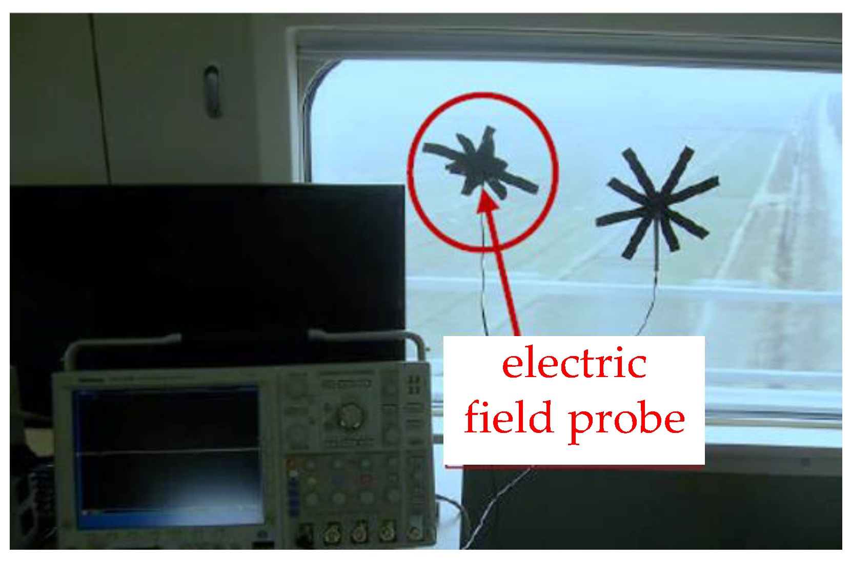
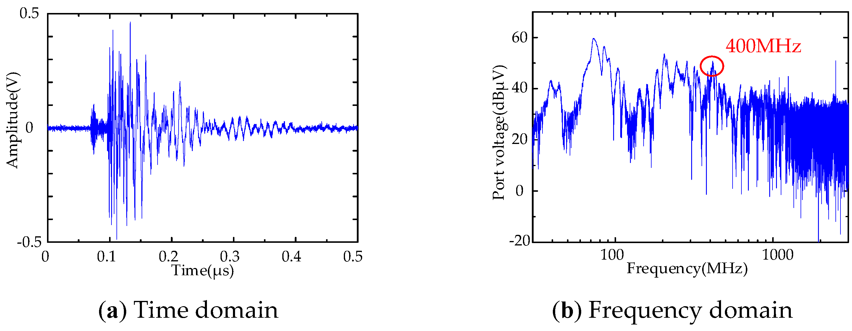
2.1. Pantograph Arcing Signal Collection

Field measurements of electromagnetic disturbance induced by off-line discharges of the grid mainly refer to measuring the time-domain waveform of the radiation field through an antenna or an electric field probe on a railway site, and then analyzing its radiation properties. The measurement instruments used are shown in

Table 1. Basic parameters of the instruments and equipment required for field measurements.

Instrument	Model Number	Performance
digital storage oscilloscope	Tektronix TDS3052	500 MHz, 5 GS/s
electric field probe	HI-6105	100 kHz–6 GHz

, and the test layout and installation locations of the broadband electric field probe are shown in Figure 1.

As can be seen from Figure 2, the single pantograph arcing signal is composed of a series of oscillating and attenuating pulses in the time domain. The rising edge time is at ns level and the duration is within 1 μs. The radiation disturbance caused by pantograph arcing is a wide-frequency electromagnetic field, ranging from tens of kHz to a few GHz, with the main power spectrum concentrated at a few hundred MHz. According to China’s frequency planning and usage, 400 MHz is available for the LTE-R system. At 400 MHz, the field strength is about 47 dBμV/m. However, there are some differences in the pulse signal data for each measurement, which have strong randomness. Therefore, it is not accurate to analyze the impact of the LTE-R system using only the results of one measurement.

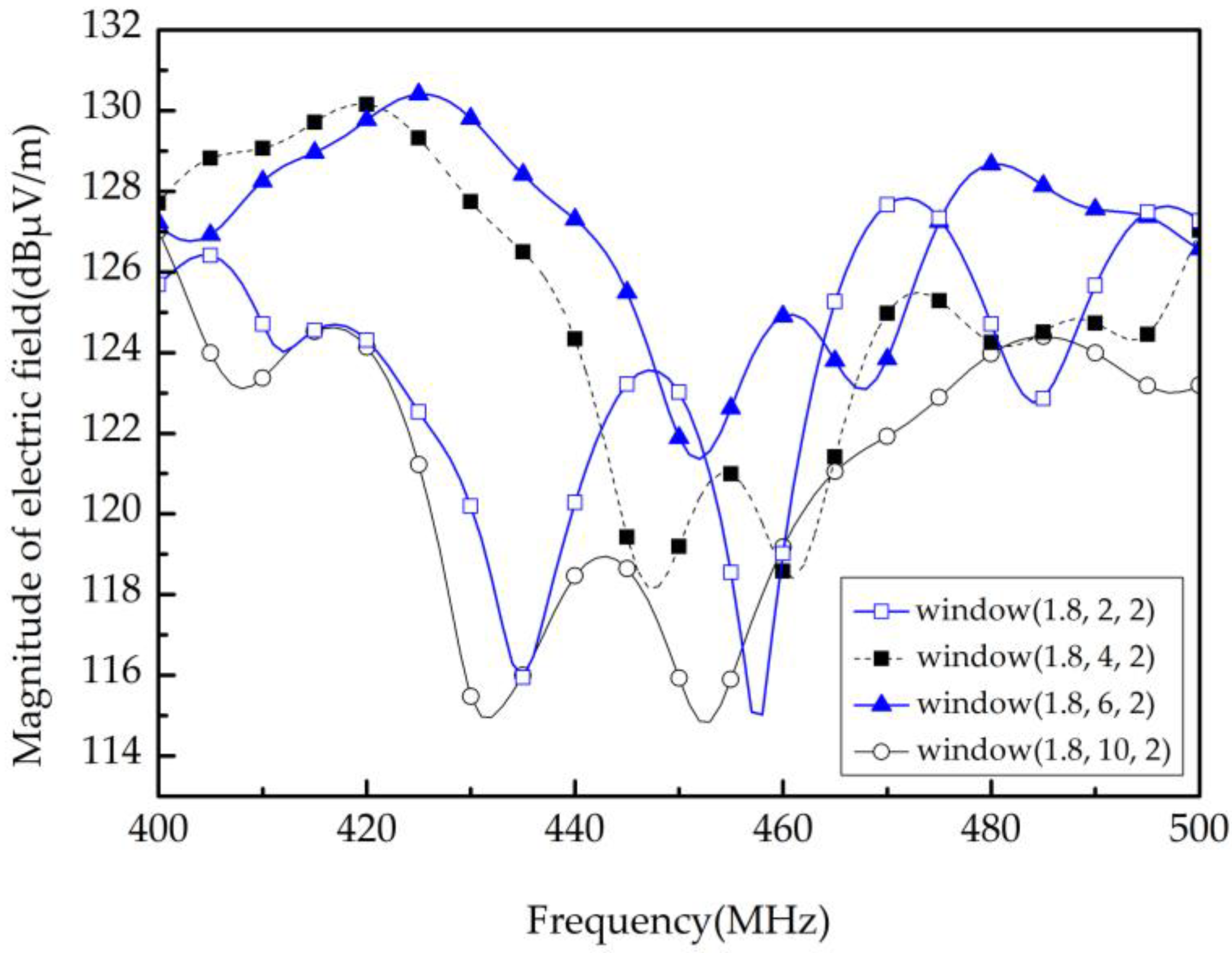
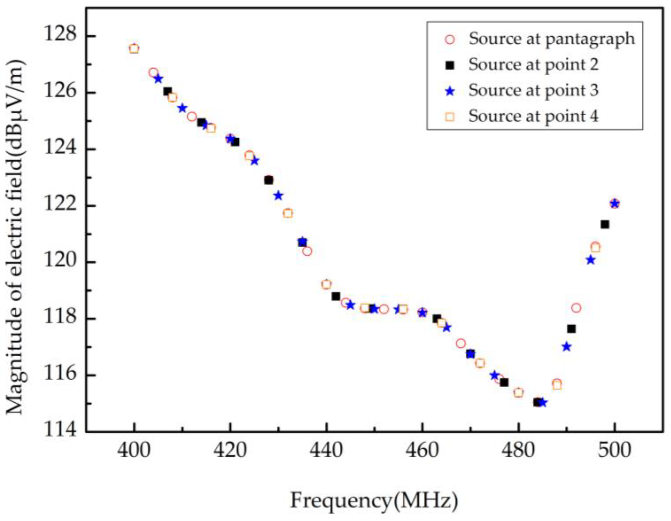
2.2. The Effect of Measuring Position

Due to the propagation of the radio waves and the effect of the carriage, the electromagnetic field of the pantograph arcing is different at different locations. What is to be done is to use the pantograph arcing field data wherever they are obtained. Thus, a simulation model is built to get the electric field data at the window. In addition, the data could be used to find the coupling relationship between the probe at the window and the LTE-R roof antenna. Therefore, the electric field data of measurement can be used to analyze the electromagnetic response of the LTE-R system.

Due to limitations in the size and simulation time of the electromagnetic simulation, only two carriages are considered, as shown in Figure 3. The source is located at the position of the pantograph. The probe at the window measures the effect of the measurement position on the field. The antenna on the roof measures the field received by the LTE-R antenna.

The disturbance source used in the model is a Gaussian pulse. The maximum magnitude of the source is 1A. The frequency range is from 400 MHz to 500 MHz, which is the band where LTE-R antennas mostly operate. Four window locations are selected to obtain field data. The position is defined as (x, y, z) with the unit m, where x is the distance from the pantograph to the probe of the window at x direction, y is the distance from the pantograph to the probe of the window at y direction and z is the distance from the pantograph to the probe of the window at z direction. The four window positions are point 1 (1.8, 2, 2), point 2 (1.8, 4, 2), point 3 (1.8, 6, 2), and point 4 (1.8, 10, 2). As the size of the carriage is fixed, the position of the probe at x direction is fixed.

As can be seen from Figure 4, the electric fields at the same position are different for different frequencies. At the same frequency, it varies with different measurement positions. Theoretically, at the same frequency, the electric field strength will decay linearly with the probe position. In fact, the electric field strength does not decay with the position of the probe due to the electric field distribution being affected by the carriage of the train. For example, the magnitude of the electric field strength at point 2 is larger than that at other points at 400 MHz.

Then, the source location is changed to three additional positions of the window, point 2 (1.8, 4, 2), point 3 (1.8, 6, 2), and point 4 (1.8, 10, 2). The electric field received by the antenna is compared with the electric field received when the source is at the position of the pantograph. The results are shown in Figure 5. The electric fields at the roof antenna position are the same. The magnitude of the electric fields does not change with the change of the probe coordinate at the viewing position of the window. It indicates that the variation of the electric field probe position of the window does not affect the radiation coupling path of the pantograph arcing signal to the antenna port. The electric field measurement data at the window are an intermediate variable to analyze the effect of the pantograph arcing on the LTE-R system.

3. A Fast Prediction Model for the Coupling Coefficient

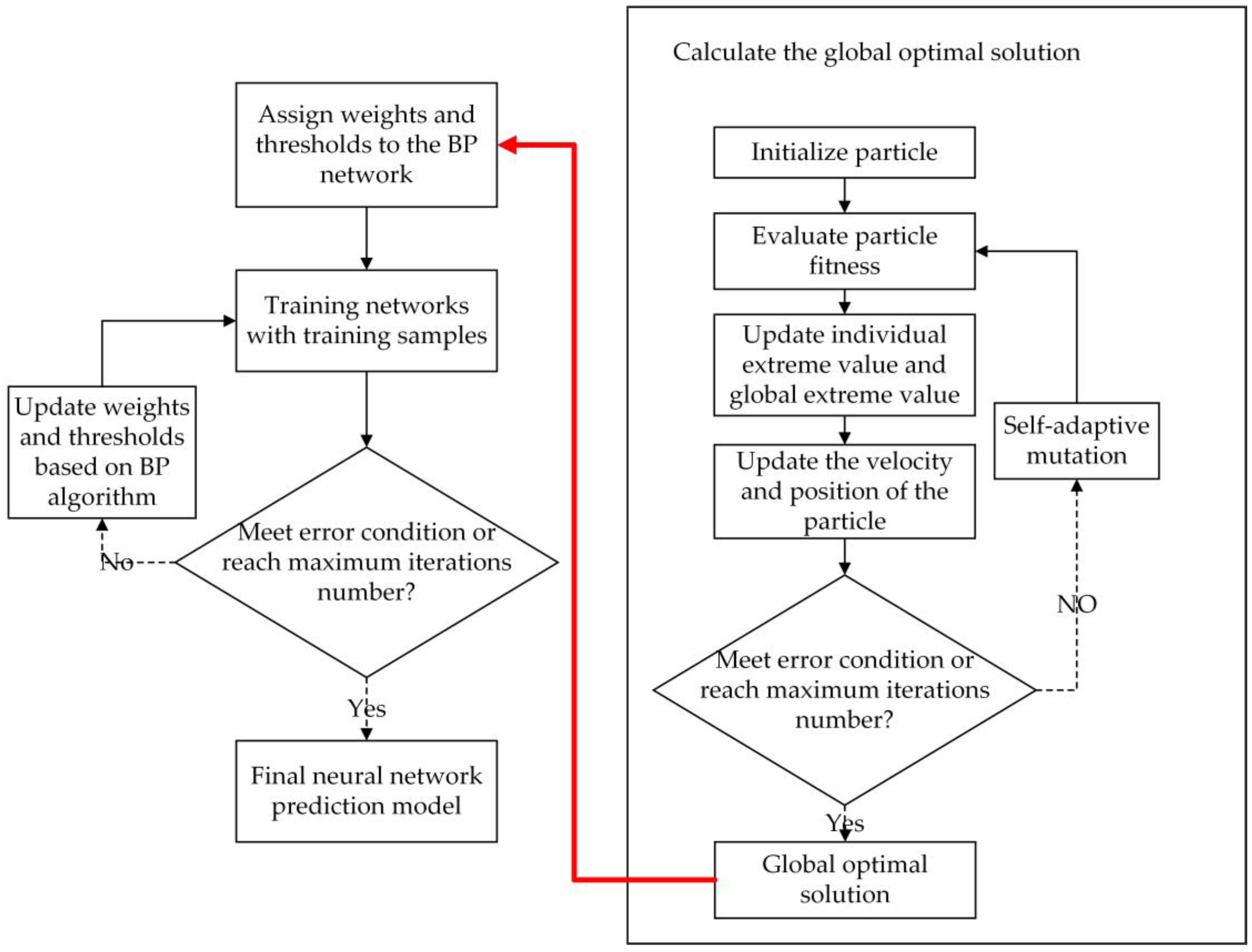
3.1. Structure and Parameters of the PSO-BP Neural Network

In the process of BP network training, it is possible to fall into the local minimum, where the amount of backpropagation training is excessive and the convergence speed of the network training is slow, which may lead to the problem of poor network model results. The PSO algorithm can be used to optimize the weights and thresholds of the BP neural network. When the BP network is trained by the PSO algorithm, the weights and thresholds between each layer of neuron nodes in the neural network structure are encoded into a particle swarm. The fitness value is the mean squared error of the network output. First, the weight and threshold vector is initialized and then the PSO algorithm is used to search for the optimal result, that is, the weights of the neuron nodes of each layer are searched within a defined number of iterations to minimize the output mean squared error of the network structure. The specific steps are:

(1)

Initialize each particle and randomly generate velocity and position vectors.

(2)

Evaluate the fitness of each particle.

(3)

Update the individual extreme value and global extreme value of each particle.

(4)

Update the velocity and position of the particle.

(5)

Determine the convergence. If the given error is reached, the next iteration is carried out. If the given error is not satisfied, the previous step is returned until the maximum number of iterations is reached.

(6)

Output the optimal solution.

In [17], the specific description of the PSO algorithm is as follows: in the continuous space, assuming that M is the population size of the particle swarm, the position of particle i at time t in coordinates can be expressed as X_i^t = (x_i1^t, x_i2^t, …, x_im^t), i = 1, 2, …, M. The velocity of particle i is the displacement of each iteration, expressed as V_i^t = (v_i1^t, v_i2^t, …, v_im^t), i = 1, 2, …, M. The velocity and position of particle i at time t are updated according to the following formulas:

$$v_{id}^t=w{v}_{id}^{t-1}+c_1{\tau }_1(p_{i}d-x_{id}^{t-1})+c_2{\tau }_2(g_d-x_{id}^{t-1}),$$

(1)

$$x_{id}^t=x_{id}^{t-1}+v_{id}^t,$$

(2)

where w is the weighted inertia value, which is used to indicate the degree of retention with the original velocity. The higher the value, the more the velocity of the particle is affected by the velocity of the previous generation. c₁ is the acceleration factor, which is the coefficient that tracks its own historical optimum. c₂ is the acceleration factor, which indicates the learning degree of the current particle for the global optimal particle. τ₁ and τ₂ are randomly generated positive numbers less than 1. p_i is the historical optimal value of the current particle and g_d is the historical optimal value of the global particle. v_id^t−1 is the velocity of the (t − 1) iteration of the particle. (p_id − x_id^t−1) is the particle’s knowledge of itself, which is used to guide the particle to move to the best position in its own history, constantly pushing the particle to reduce the error. (g_d − x_id^t−1) is the embodiment of individual cooperation in the particle swarm, where each particle guides all particles in the swarm to seek the global optimal solution by sharing information.

In summary, the specific flow block diagram of the PSO-BP neural network model algorithm is shown in Figure 6.

In this paper, the PSO-BP neural network is trained. The parameters of the PSO-BP algorithm are given in

Table 2. Parameters of the PSO-BP algorithm.

Parameters	Value
Acceleration factor c1	2.49445
Acceleration factor c2	2.49445
Number of iterations	300
Maximum velocity	1
Minimum velocity	−1
Maximum position	5
Minimum position	−5

. The PSO-BP neural network topology is shown in Figure 7. The input dimension of network I is 3 and the output dimension is 1. The input dimension of network II is 4 and the output dimension is 1. The number of neurons in the hidden layer of the two networks is 4. The Tansig function is used as an activation function. The number of training epochs is set to 500, the learning rate is 0.1, and the minimum error of the training objective is 0.00001.

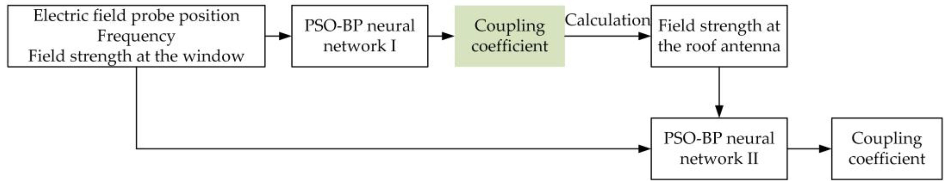
3.2. Structure of the Cascade PSO-BP Neural Network

A cascade neural network can combine multiple networks of the same kind or different networks into a multi-layer structure, with the advantages of a fast learning speed and no need for the backward propagation of error signals. The cascade neural network model established in this paper is composed of two identical PSO-BP networks. The main structure of the prediction model is shown in Figure 8.

In the PSO-BP cascade neural network model, neural network I does not directly input into neural network II, but instead calculates the electric field strength at the roof antenna through the coupling coefficient. The field strength at the roof antenna is calculated by Equation (3):

S = E_r − E_w

(3)

where E_r is the electric field strength at the roof antenna, in dBμV/m; E_w is the electric field strength at the window, in dBμV/m; S is the coupling coefficient, defined as the ratio of the electric field strength at the roof antenna to the electric field strength at the window. The electric field strength at the roof antenna is used as the input to neural network II. At the same time, the input of neural network I is also used as the input of neural network II to predict the coupling coefficient of the electric field strength between the window position and the roof antenna port. This means that there are three steps in the model construction process.

For the first step, the model in Figure 3 is used to obtain the field data. The antenna position is assumed to be constant and the window probe position is varied by 1 m in the y direction and 0.4 m in the z direction. The dataset is then pre-processed to extract feature components, which are used as inputs into the neural network model. In this paper, 80 percent of the data from the above sample set is randomly selected as the training set, and the remaining 20 percent is used as the validation set. The training set data is used to train the PSO-BP neural network I, which is validated by the validation set.

In the second step, the measured field data received by the window probe is used to predict the coupling coefficient with the PSO-BP neural network I, and the field strength at the roof antenna is calculated. The field strength at the roof antenna is the input of the PSO-BP neural network II.

The third step is to train the PSO-BP neural network II. The input data contains both simulation data and measurement data. This will improve the accuracy of the model. The output of the PSO-BP neural network II is the coupling coefficient. Similarly, the electric field strength at the roof antenna is calculated using Equation (3).

By further comparing and analyzing the prediction results of the proposed cascade neural network with a single neural network, it can be concluded that the prediction accuracy of the cascade neural network prediction model is significantly improved. The specific analysis of the prediction results will be given below.

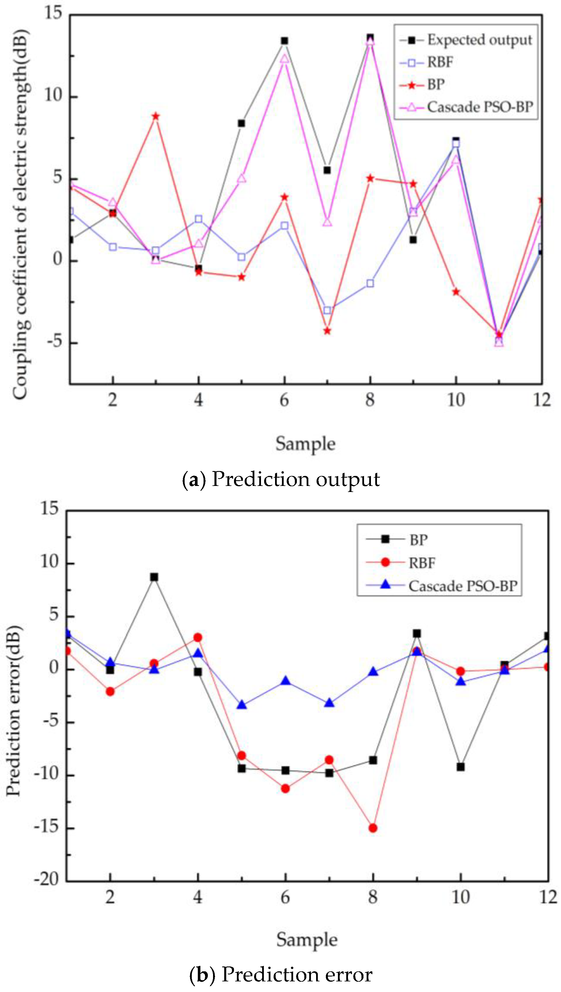
3.3. Prediction Results and Errors

Electromagnetic simulations are performed to obtain the electric field strength at the window and the LTE-R fixed antenna on the roof. After data preprocessing, a nonlinear relationship between the coupling coefficient and the spatial coordinate, frequency, and average electric field strength at 400 MHz–500 MHz at the window and the roof is established. The prediction output, the prediction error of the proposed cascade network model based on the PSO-BP algorithm, is shown in Figure 9. The prediction output and prediction error are also compared with those of a single BP neural network model or a single RBF (Radial Basis Function) neural network model. From Figure 9a, the proposed cascade PSO-BP model is closest to the expected output. Further, according to Figure 9b and

Table 3. The maximum error of three prediction results.

Neural Network Model	Maximum Error (dB)
BP	9.8
RBF	15.2
PSO-BP	3.6

, the maximum error of the predictions of the three network models is shown: the BP and RBF neural network models have relatively large errors, reaching 9.8 dB and 15.2 dB, respectively. The prediction accuracy of the two models, in this case, needs to be improved. Therefore, the neural network model is modified and the proposed cascade PSO-BP neural network is introduced, which effectively reduces the prediction error to 3.6 dB. The accuracy of the prediction results is significantly improved, which meets the uncertainty requirements in measurement. Based on the predicted coupling coefficient, the disturbance electric field strength at the roof antenna can be calculated from the electric field strength at the window position, and the electromagnetic response coupled to the antenna port when the pantograph arcing occurs can be quickly predicted.

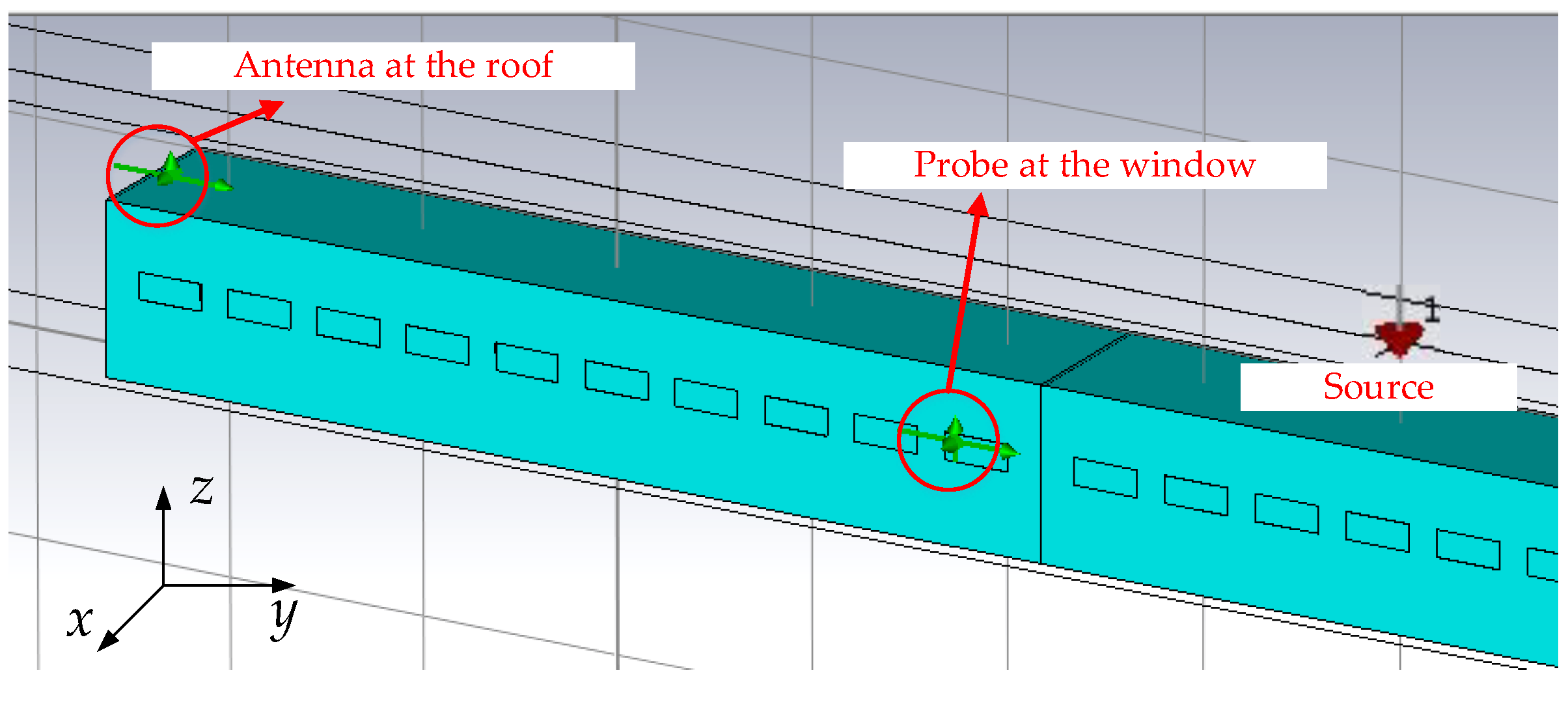
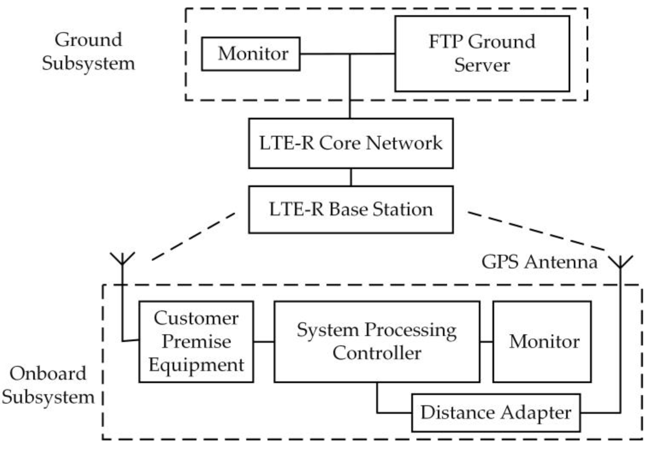
4. Analysis of the Electromagnetic Interference Induced by the Coupling of the Pantograph Arcing to the LTE-R Roof Antenna

In this section, the model of the LTE downlink physical layer is simulated in MATLAB, and simulation metrics including throughput and block error rates are introduced. A detailed analysis of the impact of the pantograph arcing interference on LTE-R communication quality has been performed and verified by field measurements.

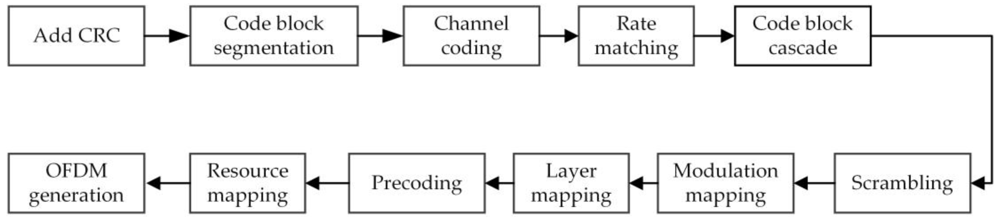
4.1. Simulation of the LTE-R Downlink Physical Layer

According to references [18,19], the model of the physical layer of LTE-R downlink is established, as shown in Figure 10.

The PDSCH (Physical Downlink Shared Channel) is selected for the LTE-R downlink simulation model in this paper, and the basic simulation parameters are set as shown in

Table 4. Basic Parameters for the Downlink Simulation.

Parameters	Description
Duplexing mode	FDD
CP length	normal
Carrier frequency	400 MHz
Modulation scheme	64 QAM
Bandwidth	5 MHz, 10 MHz, 20 MHz
Code rate	1/3
Number of users	1
CFI	1
Signal channel	AWGN

.

In [10], the simulated electric field of discharge radiation disturbance at the receiving antenna is added to the simulated LTE-R transmission channel, and the received signal can be expressed as Equation (4):

$$E_R(t)=E_{LTE}(t)+E_i(t),$$

(4)

where E_i(t) is the disturbance signal received by the LTE-R antenna, and E_LTE(t) is the LTE-R signal, which can be expressed as Equation (5):

$$E_{LTE}(t)=E_{LTE\_I}(t)\cos (2\pi f_{c}t)-E_{LTE\_Q}(t)\sin (2\pi f_{c}t),$$

(5)

where E_{LTE_I}(t) and E_{LTE_Q}(t) are isotropic and orthogonal components.

In this paper, BLER (Block Error Rate) and throughput are used to evaluate the interference degree of the communication link.

BLER is the requirement of RLC (Radio Link Control) for error retransmission, which is used for measuring the reliability of digital communication systems. It is defined as the ratio of the number of error transmission blocks to the total number of transmission blocks received by the system. Throughput, a fundamental indicator of the wireless performance of LTE networks, refers to the number of bits successfully transmitted under the condition that the delay requirement per second is satisfied, which can be obtained from Equation (6):

$$Througtput=R\cdot (\frac{1-BLER}{\overline{N}}),$$

(6)

where R is the data rate transmitted by wireless base stations and $\stackrel{-}{N}$ is the average number of data transfers per frame, defined as the ratio of the total number of data transfers to the total number of frames sent [20].

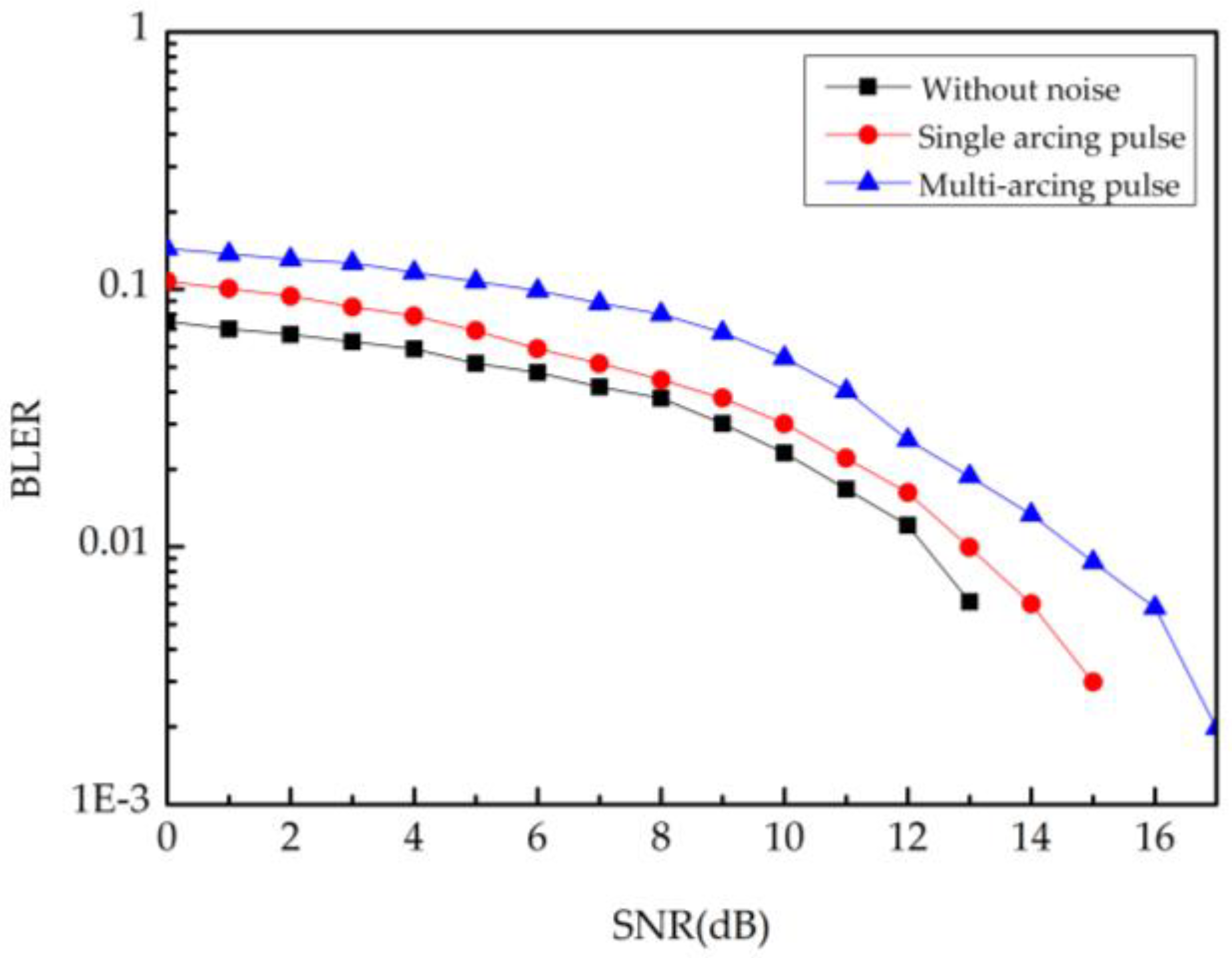
4.2. Interference Analysis of LTE-R System

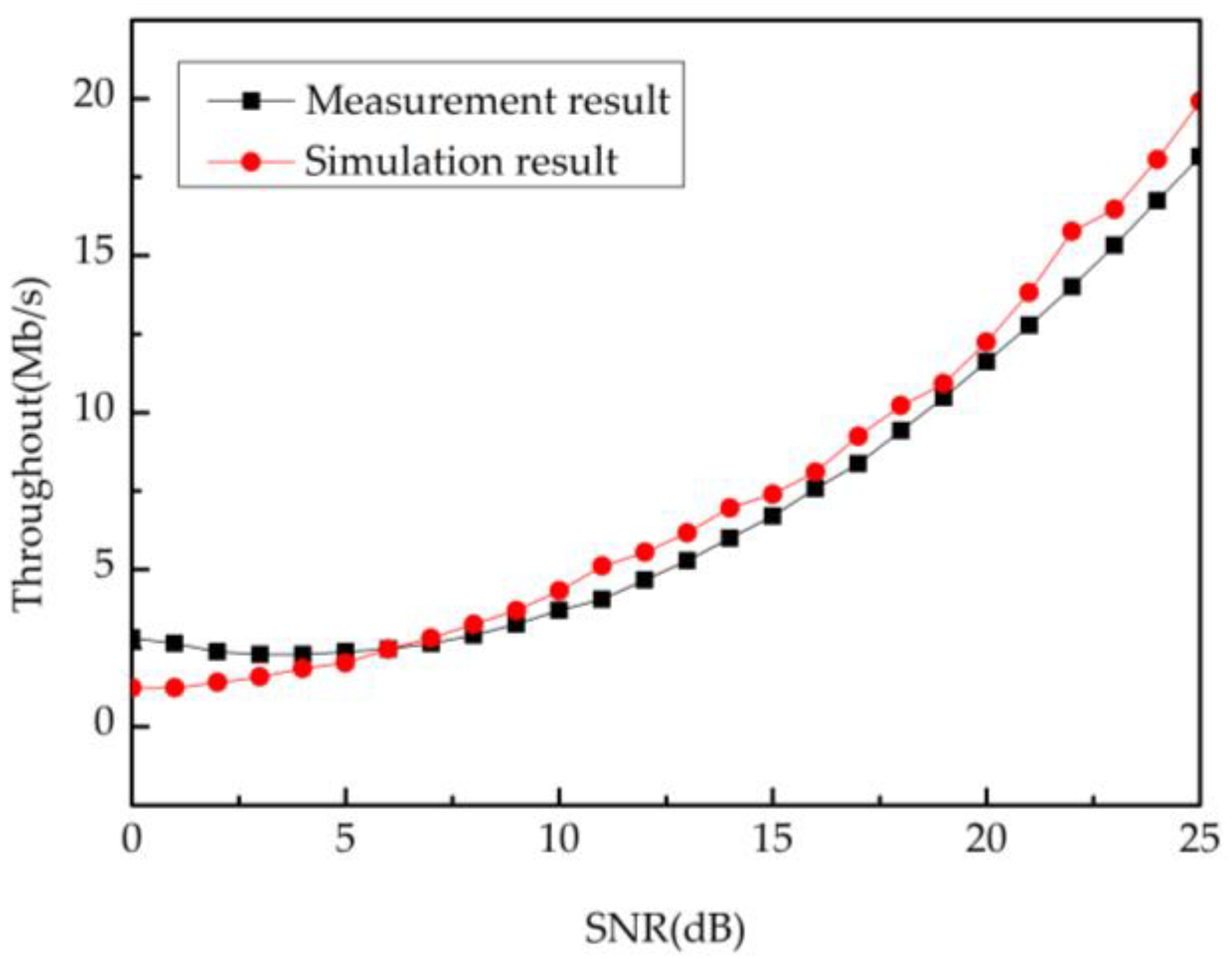
The result of the BLER varies with the SNR (Signal-to-Noise Ratio) and is shown in Figure 11. The result of throughput varies with SNR and is shown in Figure 12.

$$\mathrm{SNR}=E_b/N_0,$$

(7)

where E_b is the signal energy per bit and N₀ is the white Gaussian noise power of the channel.

As shown in Figure 11, the BLER of the LTE-R system with added noise increases significantly when the SNR is in the range of 0 dB–17 dB. After adding the single arcing pulse signal, the BLER is less than 10⁻¹ when the SNR is greater than 0 dB. However, after adding the multi-arcing pulse signal, the BLER is less than 10⁻¹ when the SNR is greater than 6 dB. It indicates that the LTE-R system is affected more by the multi-arcing pulse signal. Moreover, as the SNR increases, the BLER after adding noise eventually decreases to the order of 10⁻³. In other words, in the presence of poor SNR conditions, pantograph arcing radiation noise can lead to an increase in the BLER, resulting in an increase in the probability of system disruption.

According to the performance requirements of the 3 GPP (3rd Generation Partnership Project) for LTE systems, when the BLER is less than 10 percent, the system can meet the service reliability requirements. The LTE system can improve the decoding accuracy rate through the HARQ (Hybrid Automatic Repeat Request) retransmission process, so that the BLER is gradually lower than 10⁻¹. However, an increase in the number of retransmissions leads to a decrease in the system throughput and decoding gain.

As shown in Figure 12, compared to the noiseless case, the throughput is reduced by an average of 8% in the SNR range below 18 dB and by an average of 2.9% in the SNR range above 18 dB and below 25 dB after the addition of a single arcing pulse signal. After adding the multi-arcing pulse signal, the throughput is reduced by an average of 20% in the SNR range below 16 dB and by an average of 9% in the SNR range above 16 dB and below 25 dB. Combining this with Figure 11, it can be concluded that when the BLER is high, the system will increase the retransmission, leading to a decrease in the effective throughput. However, as the SNR gradually increases, the effect of noise on the throughput gradually decreases, but the effect of the multi-arcing pulse is greater than that of a single-arcing pulse.

Therefore, pantograph arcing can affect LTE-R communication quality at 400 MHz and affect transmission reliability when the SNR is poor. It generally leads to a reduction in throughput and a reduction in service data transmission. In general, this will result in a reduction in throughput and data transmission for the service.

4.3. Verification

In [20], researchers conducted on-site measurements of the throughput of LTE-R systems based on the File Transfer Protocol (FTP) under high-speed conditions. The equipment connection of the measurement system is shown in Figure 13. FTP transmits 100 MB of files between the onboard subsystem and the ground subsystem as the train travels through the LTE-R network coverage area at high speed. The control part of the terminal side calculates the peak downlink throughput, which is the maximum amount of data that can be transmitted per second, to obtain the relationship between downlink throughput and SNR. The simulation data are compared with the field measurement data in Figure 14.

It can be seen that the field measurements are in good agreement with the simulations. The downlink throughput increases as the SNR increases. When the SNR is within the range of 0 dB–25 dB, the maximum throughput can reach 19.9 Mbps, which is 53.2% lower than the theoretical value of the 42.5 Mb/s downlink peak rate calculated in [21].

5. Conclusions

In this paper, a fast prediction model based on machine learning is developed to accurately and quickly predict the electromagnetic response of onboard equipment at a certain location. This approach applies a cascade neural network model based on PSO-BP to predict the electromagnetic interference at the LTE-R antenna. It avoids the problems of difficult operation in field measurements for the LTE-R system. A good agreement can be found between the measurements and the proposed methodology. The results show that pantograph arcing will lead to an increase in the BLER of the LTE-R system at 400 MHz. System performance and transmission efficiency will be affected. However, the simulation model is a simplified one. The structure of the body of the carriage is equivalent to a rectangular structure in the model. In order to further improve the prediction accuracy, the structure could be optimized.

References

1. Ma, L. The Radiated Characteristics of Pantograph Arcing in High-Speed Railway. Ph.D. Thesis, Beijing Jiaotong University, Beijing, China, 2018. [Google Scholar]
2. He, W. Analysis of EMI Caused by Arcs in Pantograph-Catenery Systems and Study of Realizing the Measure System. Master’s Thesis, Southwest Jiaotong University, Chengdu, China, 2012. [Google Scholar]
3. Mariscotti, A.; Marrese, A.; Pasquino, N. Time and frequency characterization of radiated disturbances in telecommunication bands due to pantograph arcing. In Proceedings of the Instrumentation & Measurement Technology Conference, Graz, Austria, 13–16 May 2012; pp. 2178–2182. [Google Scholar]
4. Fridhi, H.; Deniau, V.; Ghys, J.P.; Heddebaut, M.; Rodriguez, J.; Adin, I. Analysis of the Coupling Path between Transient EM Interferences Produced by the Catenary-pantograph Contact and On-board Railway Communication Antennas. In Proceedings of the International Conference on Electromagnetics in Advanced Applications, Turin, Italy, 9–13 September 2013; pp. 587–590. [Google Scholar]
5. Dudoyer, S.; Deniau, V.; Adriano, R.R.; Slimen, M.N.B.; Rioult, J.; Meyniel, B.; Berbineau, M. Study of the Susceptibility of the GSM-R Communications Face to the Electromagnetic Interferences of the Rail Environment. IEEE Trans. Electromagn. Compat. 2012, 54, 667–676. [Google Scholar] [CrossRef]
6. Xia, Y. The Evolution of Railway Wireless Communication Technology towards LTE-R. Chin. Railw. 2012, 8, 2. [Google Scholar]
7. Yin, X.L. Technical Analysis of LTE-R Application in Chinese Railways. Railw. Technol. Superv. 2016, 44, 40–44. [Google Scholar]
8. Zhang, Y. A Brief Talk on the Development and Evolution of Railway Communication System to LTE-R. Railw. Commun. Signal Eng. Technol. 2016, 13, 3. [Google Scholar]
9. Stienne, O.; Deniau, V.; Simon, E.P. Assessment of transient EMI impact on LTE communications using EVM & PAPR. IEEE Access 2020, 8, 227304–227312. [Google Scholar]
10. Wang, J.; Wang, G.; Zhang, D.; Zhang, J.; Wen, Y. The Influence of Pantograph Arcing Radiation Disturbance on LTE-R. In Proceedings of the 2019 International Conference on Electromagnetics in Advanced Applications, Granada, Spain, 9–13 September 2019; pp. 0583–0586. [Google Scholar]
11. Wang, Y.; Zhang, X.; Zhu, G.; Lin, S.; Wang, W. Evaluation of LTE-R System Performance with Pantograph-Catenary Arc Interference. In Proceedings of the 2020 IEEE International Symposium on Antennas and Propagation and North American Radio Science Meeting, Montreal, QC, Canada, 5–10 July 2020; pp. 1277–1278. [Google Scholar]
12. Song, Y.; Wen, Y.; Zhang, D.; Lin, S.; Wang, W. Fast Prediction Model of Coupling Coefficient Between Pantograph Arcing and GSM-R Antenna. IEEE Trans. Veh. Technol. 2020, 69, 11612–11618. [Google Scholar] [CrossRef]
13. Song, Y.; Wen, Y.; Zhang, J.; Zhang, D. Fast Prediction Model for the Susceptibility of Balise Transmission Module System Based on Neural Network. In Proceedings of the 2019 International Conference on Electromagnetics in Advanced Applications, Granada, Spain, 9–13 September 2019; pp. 0445–0448. [Google Scholar]
14. Li, Q.; Zhou, K.X. The Research of the Pressure Sensor Temperature Compensation Based on PSO-BP Algorithm. Acta Electron. Sin. 2015, 43, 412–416. [Google Scholar]
15. Liu, S.; Zhao, Y.; Zhang, W.; Zhao, X.; Chen, Z. Research on Stranding Crosstalk Prediction Based on PSO-BP Neural Network Algorithm. Electr. Autom. 2023, 45, 52–54. [Google Scholar]
16. Tang, X.; Shi, L.; Wang, B.; Cheng, A. Weight Adaptive Path Tracking Control for Autonomous Vehicles Based on PSO-BP Neural Network. Sensors 2022, 23, 412. [Google Scholar] [CrossRef] [PubMed]
17. Zhao, L.; Yang, Y. PSO-based single multiplicative neuron model for time series prediction. Expert Syst. Appl. 2008, 36, 2805–2812. [Google Scholar] [CrossRef]
18. 3GPP TS 36.211 v8.6.0-2009; Evolved Universal Terrestrial Radio Access (E-UTRA) Physical Channel and Modulation (Release 8). ETSI: Valbonne-Sophia Antipolis, France, 2009.
19. 3GPP TS 36.212 v9.0.0-2009; Evolved Universal Terrestrial Radio Access (E-UTRA) Multiplexing and Channel Coding (Release 9). ETSI: Valbonne-Sophia Antipolis, France, 2009.
20. Alouini, M.S.; Goldsmith, A. Area spectral efficiency of cellular mobile radio systems. IEEE Trans. Veh. Technol. 1999, 48, 1047–1066. [Google Scholar] [CrossRef]
21. Li, C.D. Research on High Speed Adaptability of Railway LTE-R Broadband Mobile Communication System. Master’s Thesis, China Academy of Railway Sciences, Beijing, China, 2019. [Google Scholar]
Figure 1. Test layout.
Applsci 13 06640 g001
Figure 2. Pantograph arcing measured at the site.
Applsci 13 06640 g002
Figure 3. Model of the electric field simulation.
Applsci 13 06640 g003
Figure 4. The magnitude of the electric field at the window of the carriage.
Applsci 13 06640 g004
Figure 5. The electric field measured by the antenna on the roof.
Applsci 13 06640 g005
Figure 6. The specific flow block diagram of the PSO-BP neural network.
Applsci 13 06640 g006
Figure 7. PSO-BP neural network topology.
Applsci 13 06640 g007
Figure 8. Structure of the proposed cascade neural network prediction model.
Applsci 13 06640 g008
Figure 9. Prediction output and error of the three neural network models.
Applsci 13 06640 g009
Figure 10. Link flow of the physical layer of LTE-R downlink.
Applsci 13 06640 g010
Figure 11. BLER varies with SNR.
Applsci 13 06640 g011
Figure 12. Throughput varies with SNR.
Applsci 13 06640 g012
Figure 13. Equipment connections for the throughput measurement system.
Applsci 13 06640 g013
Figure 14. Scatter plot of the downlink throughput and SNR.
Applsci 13 06640 g014