Effective and Interpretable Rule Mining for Dynamic Job-Shop Scheduling via Improved Gene Expression Programming with Feature Selection

Abstract

Gene expression programming (GEP) is frequently used to create intelligent dispatching rules for job-shop scheduling. The proper selection of the terminal set is a critical factor for the success of GEP. However, there are various job features and machine features that can be included in the terminal sets to capture the different characteristics of the job-shop state. Moreover, the importance of features in the terminal set varies greatly between scenarios. The irrelevant and redundant features may lead to high computational requirements and increased difficulty in interpreting generated rules. Consequently, a feature selection approach for evolving dispatching rules with improved GEP has been proposed, so as to select the proper terminal set for different dynamic job-shop scenarios. First, the adaptive variable neighborhood search algorithm was embedded into the GEP to obtain a diverse set of good rules for job-shop scenarios. Secondly, based on the fitness of the good rules and the contribution of features to the rules, a weighted voting ranking method was used to select features from the terminal set. The proposed approach was then compared with GEP-based algorithms and benchmark rules in the different job-shop conditions and scheduling objectives. The experimentally obtained results illustrated that the performance of the dispatching rules generated using the improved GEP algorithm after the feature selection process was better than that of both the baseline dispatching rules and the baseline GEP algorithm.

1. Introduction

Production scheduling is a practical and significant problem that reflects real-world problems and difficulties in several application areas, including production planning, logistics, order processing, and others. Effective production scheduling is a critical task for manufacturing industries in order to minimize production costs and maximize resource utilization. There are two primary strands of research on production scheduling literature; the first concerns static scheduling issues, where all information about tasks is known before the start of the first task. Earlier research has been aimed at finding the most effective methods to address static scheduling issues. As product demand has continued to shift towards personalization, manufacturing processes have become more diverse, and practical scheduling problems have become more complex. Uncertainty has increased in manufacturing workshops, where such things as machine breakdowns, the arrival of urgent jobs, and changes in delivery dates can all affect the stable operation of workshops.

Among state-of-the-art methods, traditional deterministic approaches, metaheuristic algorithms, and dispatching rules are the most frequently used methods for maintaining the stability of the production process. Traditional deterministic techniques, such as branch and bound [1], dynamic programming [2], and gradient free techniques [3], are unable to handle such dynamic issues effectively and efficiently. However, it is well known that these traditional deterministic approaches are computationally expensive, and that their complexity increases exponentially with the scale of the problem. Additionally, it is extremely difficult to resolve dynamic issues that require a large number of real-time decisions. Several metaheuristics, such as particle swarm optimization [4], scatter search [5], simulated annealing [6], genetic algorithms [7], and ant colony optimization [8], have been shown to be successful and efficient in finding high-quality solutions in a reasonable amount of time. However, due to the lack of convenience and immediacy, metaheuristics have not been directly applied to real-world manufacturing.

Dispatching rules are among the most frequently applied heuristics in production scheduling due to their simplicity and ability to adapt in response to changes in the production manufacturing system. A dispatching rule can be represented as a priority function that contains data on the attributes of the jobs, the machines, or the systems. The efficiency of the dispatching rules is related to the state change in the scheduling environment [9]. Therefore, dispatching rules should be designed and generated according to the real-time changes in the production conditions in the manufacturing process. There have been plenty of dispatching rules put forth for dynamic job-shop scheduling (DJSS). More generally, the design of dispatching rules can be divided in two main ways: manual design and intelligent design. However, developing man-made dispatching rules is technically challenging, for several reasons: first, it is challenging to explore the relative importance of various job and machine features and their impact on rule performance; second, it takes a great deal of time to select and test the optimal dispatching rules using complicated modeling tests. There have been several studies advocating the use of different methodologies to design scheduling rules, and they have successfully produced rules that are far better than those constructed by hand [10,11,12]. The effectiveness of a dispatching rule relies on its capacity to account for unforeseen circumstances, as well as maximize those most crucial aspects that might impact the target [13]. While several dispatching rules have been presented, none of them can achieve optimal results in all scenarios [14]. Recently, a large number of researchers have attempted (with the help of hyperheuristics) to automatically construct dispatching rules [15].

Gene Expression Programming (GEP) is a well-known hyperheuristics approach for creating efficient scheduling heuristics for a variety of industrial applications [16,17]. Due to its powerful search engine and its ability to avoid code bloat, GEP can automatically determine the structure and parameters of the program more effectively than other artificial intelligence methods. The challenge in designing efficient dispatching rules for the GEP algorithm comes from the search space, whose size mainly depends on the tree structure, function set, and terminal set. In DJSS, the set of terminals can encompass an extensive range of features, including those that relate to the system, jobs, and machines. Prior research frequently takes into account all feasible characteristics for the development of GEP genes. Some attributes in the terminal section may not be useful and could be irrelevant or duplicative in generating optimal dispatching rules within a given job-shop context. For instance, it is believed that the due date of the job is a pointless element for minimizing mean flow time. Similarly, the weight of the job is a crucial factor to consider when the aim is to minimize mean-weighted tardiness, as opposed to mean flow time [18]. Hence, the task of identifying the crucial terminal sets for various scenarios (while ensuring that the potential regions within the search space are not neglected) presents a challenge. Feature selection in machine learning provides a good idea for solving this challenging task. Although GEP can identify relevant features and use them to evolve the best GEP trees simultaneously in the adaptive evolutionary process, there are still some relevant or redundant features. More in-depth research is needed in this area. As far as we know, few previous studies have focused on reducing the features of the terminal set when designing dispatching rules for GEP generation, and feature selection has not been considered to be a part of this evolutionary process.

Thus, we have proposed a feature selection method based on the improved GEP algorithm to deal with the low computational efficiency and slow convergence caused by the large and complex terminal sets in designing dispatching rules. Firstly, an adaptive variable neighborhood search algorithm was embedded into the GEP algorithm (IGEP) to obtain a set of excellent dispatching rules for dynamic job-shop scenarios. The IGEP methodology has been proposed with the aim of identifying optimal dispatching rules that would be capable of effectively aligning with the current job-shop scenarios. Then, based on the fitness of the best rules and the contribution of features to the rules, a weighted voting ranking method was used to select features for scenarios from the terminal set.

This study aimed to provide the following contributions:

(1) The proposal of an improved GEP method, i.e., GEP with an adaptive variable neighborhood search algorithm (IGEP), in order to mine the effective and high-quality dispatching rules for DJSS automatically. This adaptive variable neighborhood search algorithm was embedded into the GEP algorithm to further improve the exploitation ability and increase the population diversity;

(2) A weighted voting ranking method based on the contribution of each terminal to the priority function of the best rules is likewise proposed, to select features from the terminal set;

(3) A verification of the effectiveness of the suggested approach in comparison to the three GP-based algorithms and representative benchmark rules from the existing literature under mean tardiness, mean weighted tardiness, and mean flowtime objectives, respectively.

This study is structured as follows: the problem description and literature on the automated design of dispatching rules, GP/GEP-based hyperheuristics for DJSS, and feature selection approaches are reviewed in Section 2. The proposed methodology is elaborated upon in Section 3, while Section 4 provides a description of the experimental design. Section 5 covers the computational results and analysis. Finally, Section 6 presents the conclusions drawn from the study and provides recommendations for future work.

2. Background

2.1. Problem Formulation

The Dynamic Job-shop Scheduling (DJSS) issue is an example of an optimization problem, and it operates as follows: the job-shop problem is characterized by a set of $n$ jobs, denoted as $J=\left\{J_1,J_2,\cdots ,J_n\right\}$, and $m$ machines, denoted as $M=\left\{M_1,M_2,\cdots ,M_m\right\}$, at every decision point. Each job comprises a set of $n_i$ operations that must be processed in a specified sequence. Each machine can perform no more than one operation simultaneously. Each operation must be performed using a specific machine. The task involves determining an appropriate sequence of operations across all machines in order to establish an appropriate schedule at every point of decision-making. The scheduling effectiveness is evaluated using the Makespan (MS), Mean Flow Time (MFT), and Mean Weighted Tardiness (MWT). The proposed mathematical model is as follows:

Objective functions

$$\min MS=max\left\{C_{\mathrm{i}}\left|i=\mathrm{1,2},\cdots ,n\right.\right\}$$

(1)

$$\min MFT=\frac{\sum _{i=1}^n(C_i-{AT}_i)}{\left|\mathbb{C}\right|}$$

(2)

$$\min MWT=\frac{{\sum }_{i\in \mathbb{T}}{w}_i\left(C_i-D_i\right)}{\left|\mathbb{T}\right|}$$

(3)

S.T.

$$C_{i,1}-p_{i,1}\ge 0,\forall i$$

(4)

$$C_{i,j}-p_{i,j}\ge C_{i,j-1},\forall i,j$$

(5)

$${(C}_{i,j}-p_{i,j}-C_{i^{\prime },j^{\prime }})·Y_{i,j,i^{\prime },j^{\prime }}\ge 0,\forall i,i^{\prime },j,j^{\prime }$$

(6)

where, $p_{i,j}$ is the processing time of operation $O_{i,j}$, $C_{i,j}$ is the completion time of operation $O_{i,j}$, ${AT}_i$ is the arrival time of job $i$, $D_i$ is the due date of job $i$, $w_i$ is the weight of job $i$, $\left|\mathbb{C}\right|$ denotes the completed jobs, and $\mathbb{T}=\left\{i\in \mathbb{C}:C_i-d_i>0\right\}$ denotes the tardy jobs. If operation $O_{i,j}$ precedes operation ${O_{i,j}}^{\prime }$, $Y_{i,j,i^{\prime },j^{\prime }}=1$; otherwise $Y_{i,j,i^{\prime },j^{\prime }}=0$. The primary objectives (1), (2), and (3) are to minimize the makespan, mean flow time, and mean weighted tardiness, respectively. Equation (4) denotes that the starting time of the first operations of jobs must possess a non-negative value. Equation (5) guarantees that every job is executed by a single machine, exclusively. According to Equation (6), there exists a constraint that limits each machine to the processing of a single job at any given time.

2.2. Related Work

(1) Automated design of dispatching rules. Job-shop scheduling (JSS) is a combinatorial optimization problem that falls under the category of nondeterministic polynomial-time (NP) hard problems. It entails the allocation of various manufacturing tasks to machines at specific time intervals, with the aim of minimizing a set of objectives. The complexity of large-scale production issues poses challenges for the implementation of precise optimization techniques [19]. Hence, various heuristic optimization techniques, including the genetic algorithm [20], simulated annealing [21], and the ant colony algorithm [22], have been devised, to obtain near-optimal solutions for the static job-shop scheduling problem within a reasonable computational timeframe. In DJSS, it is possible for jobs to exhibit stochastic arrival patterns and their corresponding attributes may not be ascertainable prior to their arrival. Hence, conventional techniques for optimizing solutions are not feasible for dynamic scheduling problems, due to the restricted information horizon. Dispatching rules have been applied extensively to solve DJSS problems due to their computational efficiency. The reason for their widespread acceptance can be ascribed to their practical applicability, low computational complexity, and minimal information demands. In most cases, dispatching rules are regarded as a priority function, utilized to allocate priority to every job that is in the queue to be processed by a machine. Consequently, the tasks that hold the highest priority will be given precedence in processing. A large number of dispatching rules have been created by both practitioners and researchers to address diverse manufacturing conditions. Additional information can be found in various scholarly articles [23].

Dispatching rules are usually designed by experts in a tedious trial-and-error process, with candidate rules being tested in a simulation environment, modified, and retested until they fulfill the requirements for actual implementation in practice. In recent years, several researchers have suggested the automatic design of suitable dispatching rules by means of a hyperheuristic approach for JSS problems. Hyperheuristics combine the components utilized in current heuristics by different operators to build new heuristics, which are then trained on training problem cases and developed to become more successful. Regarding the automated construction of scheduling rules, it has been shown that GP is a promising hyperheuristic method, outperforming conventional machine learning techniques [24].

(2) GP/GEP-based hyperheuristic for DJSS. GP hyperheuristics have enabled the automatic evolution of high-quality heuristics, resulting in successful problem-solving outcomes in various domains, including (but not limited to) bin packing [25], cloud computing [26,27], and vehicle routing [28,29]. Burke et al. [15] proposed a classification scheme for hyperheuristic methods based on their search procedures, encompassing the selection and generation of hyperheuristics. A succinct summary of the utilization of hyperheuristics in addressing diverse scheduling and combinatorial optimization problems was also devised. According to the authors, GP is a suitable approach for adapting dispatching rules in dynamic scenarios, despite its infrequent utilization for directly addressing production scheduling issues. Branke et al. [30] designed GP algorithms with the goal of reducing mean flowtime as much as possible and demonstrating that their results are superior to those obtained using traditional dispatching rules. Karunakaran et al. [31] and Ferreira et al. [32] are the only authors to have focused on shops with stochastic processing times. However, the former did not benchmark evolving rules against existing methods, while the latter considered deterministic job arrivals. Many researchers have emphasized the significance of increasing algorithmic effectiveness. For example, surrogate models allow for quicker fitness computation. They are used to prevent the use of a substantial amount of computing time when evaluating unpromising rules. Typically, running these models is far more efficient for assessing individual fitness than running full simulations [19]. A tree-based representation has been shown to be the most effective method for developing robust scheduling heuristics in early investigations. As a consequence of their tendency to grow throughout their evolution, other representation structures have also been explored.

Gene expression programming (GEP), a kind of GP with liner representation, has been employed to design dispatching rules in a wide range of scheduling contexts, including single machine scheduling, parallel machine scheduling, job-shop scheduling, and flexible job-shop scheduling. Nie et al. [33] designed dispatching rules for dynamic single-machine scheduling issues using the GEP-based hyperheuristic method. Nie et al. [34] addressed a GEP method for flexible DJSS with job release dates by designing reactive priority rules in a linear representation. The findings demonstrated that GEP is capable of developing appropriate scheduling policies across a broad spectrum of processing circumstances and performance metrics. For dynamic multiobjective scheduling issues, Ozturk et al. [35] proposed two new approaches to extract composite scheduling rules by applying the GEP method. According to the authors, all the rules developed using GEP for this scenario outperformed the GP-evolved rules and the classical rules from the literature. Later, to construct scheduling policies for multiobjective dynamic job-shop scheduling with the constrained buffer space, Teymourfair et al. [36] employed GEP in conjunction with a simulation model, which heightened the complexity of the issue. The experimental results proved the superiority of using the GEP algorithm with the existing priority dispatching rules under different operating conditions. To address the issue of flexible job-shop scheduling problems with setup time and unpredictable work arrival, Zhang et al. [37] suggested a GEP-based dynamic scheduling technique with enhanced features. The variable neighborhood search method was employed in the survey to enhance the local search capacity of GEP, achieving superior results in comparison to the standard GEP and GP algorithms;

(3) Feature selection approaches. In dynamic job-shop situations, a diverse range of characteristics related to workshop states can be considered as potential features to be incorporated into the terminal set. It can be difficult to determine which features are advantageous for studying scheduling heuristics. Previous studies frequently incorporated any potential characteristic into the ultimate set of terminal features. The scheduling heuristics that have been designed exhibit a diverse range of characteristics, rendering them difficult to comprehend. Moreover, a significant number of terminals with redundant or irrelevant attributes can result in a search space that is both extensive and noisy, thus reducing the efficacy of the search of GP algorithms. Hence, it is essential to choose suitable terminal sets based on the practical requirements of job-shop conditions. The feature selection process is a crucial technique in the field of machine learning, as it enables the identification and selection of relevant data that can effectively reduce the exploration scope of evolutionary algorithms. As the features appearing in the evolved individual can be treated as a set of selected features, GP is considered to have the built-in feature selection ability. Determining the hidden links between a subset of features, however, is neither very efficient nor precise.

Friedlander et al. [38] suggested a feature selection methodology that relied on frequency analysis, specifically, the frequency of the occurrence of a given terminal in rules. This methodology was subject to certain constraints, whereby particular characteristics may be inaccurately assessed due to their prevalence in the redundant priority function. Therefore, Mei et al. [18] introduced an offline feature selection method for genetic programming, which evaluates the significance of features by their impact on priority functions. Despite its potential for more precise feature selection, this approach necessitates a significant investment of computational resources to generate a diverse set of high-quality individuals. Mei et al. [39] conducted a subsequent investigation wherein they developed an efficient feature selection approach that utilized both niching and surrogate techniques to generate superior dispatching rules for DJSS. One potential constraint of this study was that, despite the effectiveness of the methodology in identifying a subset of important features, the size of the evolved rules within the program remained relatively large. Nguyen et al. [14] augmented the tree-based rule representation by incorporating an attribute vector, which enhanced the interpretability of the rules by selecting important features. The primary limitation lay in its failure to account for situations wherein a particular attribute was not incorporated into the priority function. Shady et al. [40] suggested a new representation of the GP rules by modifying the attribute vector that abstracts the importance of each terminal during the evolution process. Subsequently, Shady et al. [41] expanded upon the attribute vector by incorporating it into the linear representation of GEP. This allowed for the evolution of efficient rules within simplistic structures, while remaining within reasonable computational constraints. Moreover, Panda et al. [42] proposed a new GP approach that incorporated simplification for the purpose of designing concise and efficient rules for DJSS. In addition to incorporating the conventional algebraic simplification operators, specialized numerical and behavioral simplification operators were also developed in their research. Huang et al. [43] devised scheduling tactics for multitasking problems by employing the reuse of building blocks in linear genetic programming. Fan et al. [44] used the GPHH method to solve DJSS with extended technical precedence constraints. The authors proposed a problem-specific approach for enhancing the efficacy of GP-evolved rules by integrating the job-shop state information that was pertinent to scheduling, through GP attribute selection.

In recent years, there has been a growing interest in exploring advanced techniques to improve the effectiveness and comprehensibility of the automated development of dispatching rules for Genetic Programming (GP). However, it has not been extensively studied in GEP. Furthermore, due to the extensive and complex exploration of scheduling heuristics, the identification of efficient scheduling principles represents a highly challenging undertaking. Therefore, this work aims to design interpretable and high-quality rules through an improved GEP algorithm for the DJSS problem.

3. Proposed Approach

3.1. Algorithm Framework

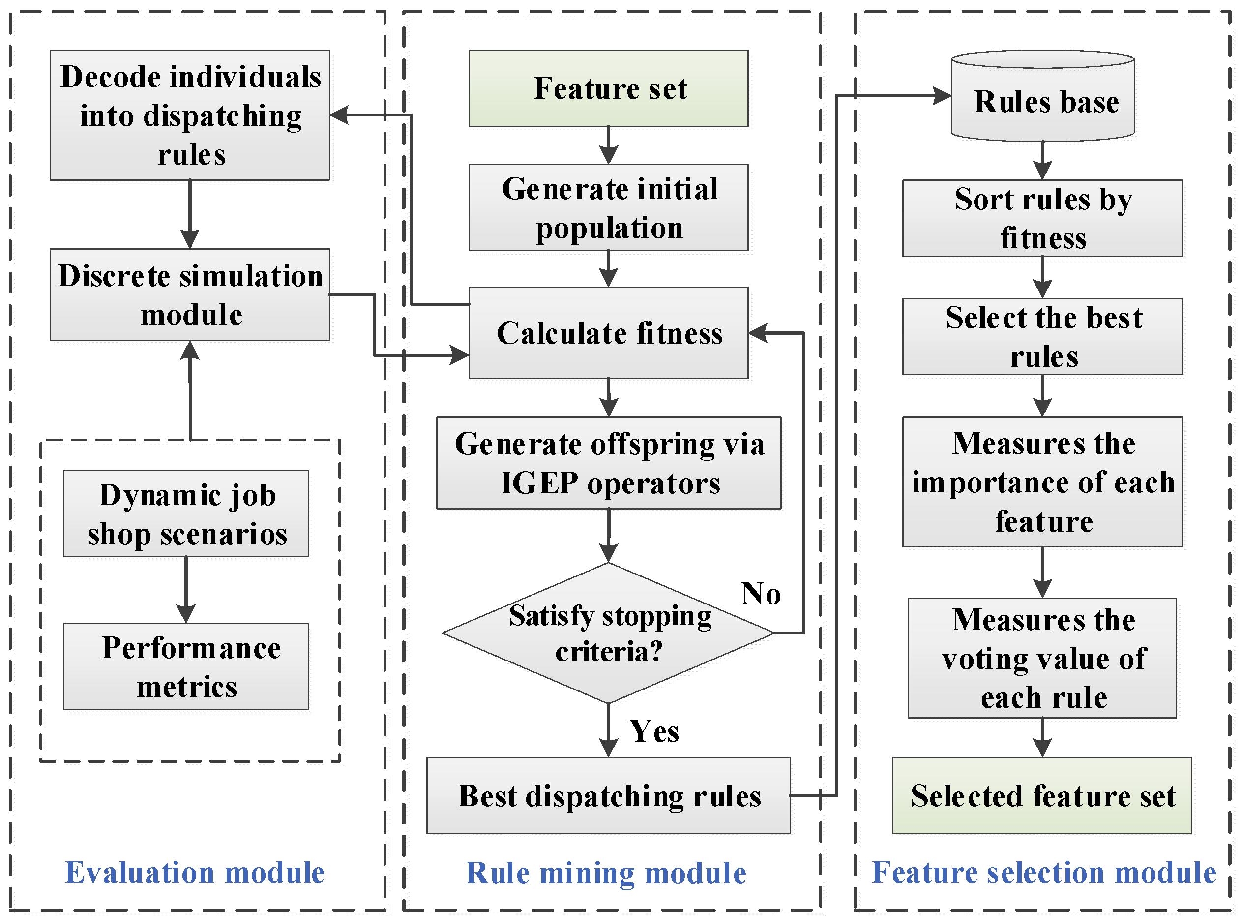
The proposed methodology comprises three distinct modules: the dispatching rule mining module, the evaluation module, and the feature selection module. Figure 1 depicts the structured framework of the proposed methodology. In the dispatching rule mining module, the GEP algorithm (integrated with an adaptive variable neighborhood search algorithm (IGEP)) is used to extract new dispatching rules by learning from the different training scenarios. The IGEP algorithm starts with an initial population, consisting of randomly generated rules. The candidate rules are subsequently presented to the evaluation model, which defines the various scheduling scenarios and assesses them, using quantitative performance metrics. After all the candidate rules are evaluated, the values of the performance measures of all rules are sent back to the dispatching rule mining module, where a new population of candidates is reproduced and modified from the current high-performing rules using genetic manipulation and a variable neighborhood search in the IGEP algorithm. Subsequently, the succeeding set of rules is transmitted to the evaluation module to assess its efficacy. This process is repeated until the stopping criteria is satisfied. In this way, the IGEP algorithm continuously searches for the optimal solution to update the rule base.

3.2. The Improved GEP

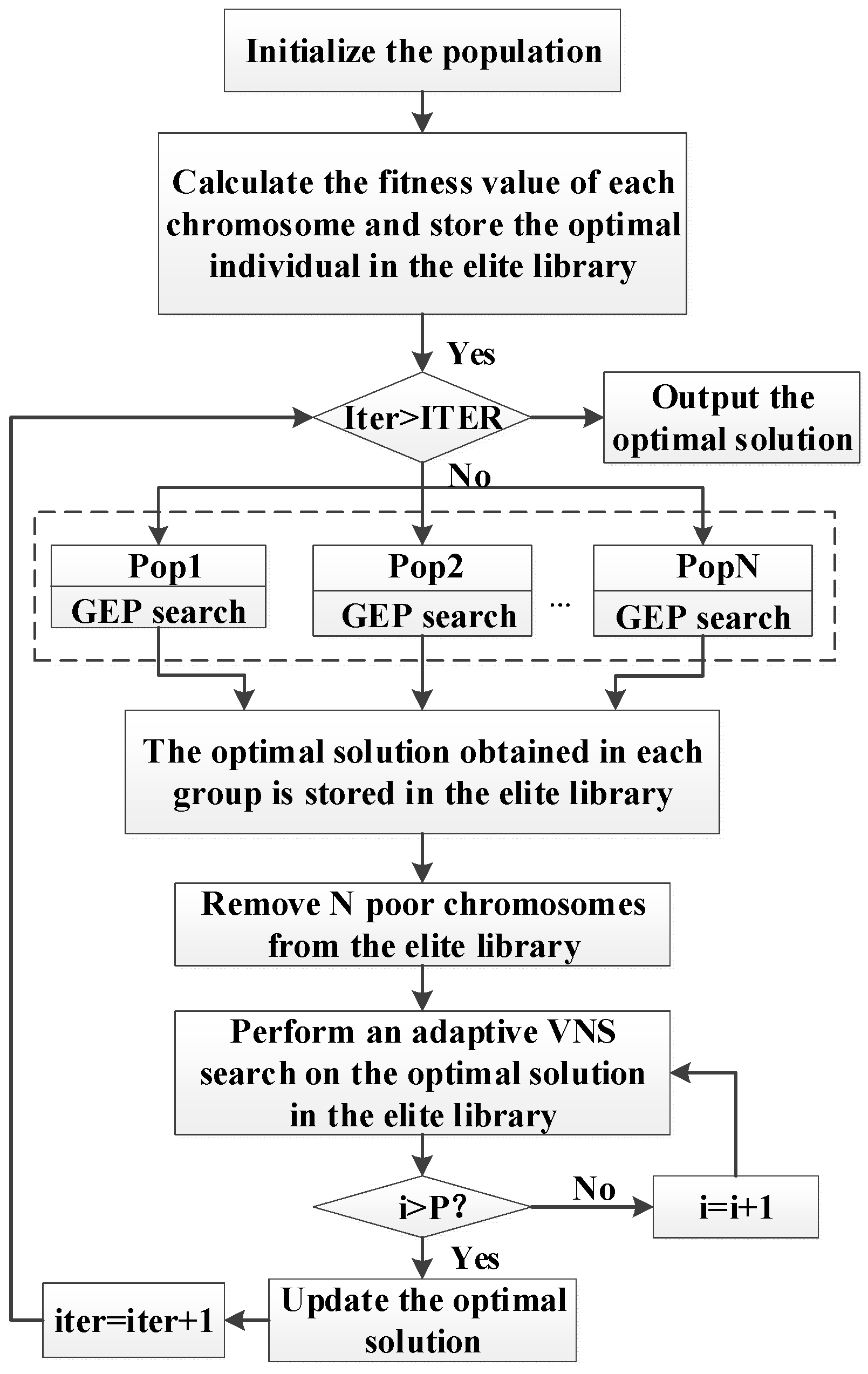
Gene expression programming (GEP) is an evolutionary computational technique invented by Ferreira for mining the dispatching rules of production scheduling. Although GEP has good global search ability during the optimization process, it was also found to have a poor local search ability. Compared with the GEP algorithm, the variable neighborhood search (VNS) algorithm has a strong ability for both local search and for search depth [45,46,47]. The VNS method employs a systematic approach to modify the neighborhood structure throughout the search process, with the aim of broadening the search space to achieve an optimal solution; that is, the initial solution can have a wider and deeper search space, which not only speeds up the approximate optimal solution of the problem, but also allows the algorithm to jump out of the local optimal solution. This paper introduces a novel VNS algorithm, incorporating an adaptive selection strategy. Unlike the conventional VNS algorithm, the proposed approach assigns a higher selection probability to superior neighborhood types based on their search performance. This enhancement leads to an improvement in both the search efficiency and search quality of the algorithm. Figure 2 depicts the flow chart of the IGEP algorithm.

3.2.1. Designing of FS and TS

The inclusion of a diverse range of job-shop characteristics, such as the remaining time of each operation and the idle time of each machine, can be considered as part of the terminal set in dynamic job-shop scheduling.

Table 1. The terminal and function sets.

Node Name	Description
AT	The current time
PT	Processing time of the operation
NPT	Processing time of the next operation
OWT	The waiting time of the operation
NOPS	Number of operations of the job
WIQ	Work in the current queue
WINQ	Work in the next queue
NOIQ	Number of operations in the current queue
NOINQ	Number of operations in the next queue
DD	Due date of the job
MRT	Ready time of the machine
SL	Slack time of the job
WKR	Work remaining (including the current operation)
NOR	Number of operations remaining
FDD	Flow due date of the operation
W	Weight of the job
Function set	+, −, ×, /, max, min

presents a comprehensive listing of the terminal and function sets. The set of terminals used in the experiments consists of common features employed in existing studies related to the GP-HH methodology [39,40,48]. The function set includes standard mathematical operators:$+,-,\times ,÷,max,min$. The operator denoted using the symbol “/” executes a protected division operation, whereby the result returned is equal to one in instances where the denominator is equal to zero.

3.2.2. Evolutionary Search Process

(1) Fitness evaluation: Fitness is crucial for GEP algorithms because it evaluates the quality of candidate solutions and directs the evolution process. The IGEP algorithm evolves a population of individuals and each one is decoded into a dispatching rule. For each specific objective, the average normalized objective value of a rule $r$ through training scenarios $S$ is taken as the rule fitness value $fitness\left(r\right)$, as shown in Equation (7), where $ref$ refers to a reference rule. The SPT/TWKR, PT + WINQ, and WATC rules are accepted as reference rules due to their remarkable performance in decreasing the MS, MFT, and MWT goals [14,18,49], respectively. Finally, Equation (8) is used to estimate the percentage change $PC$ in the performance of a given method, with respect to a reference rule:

$$fitness\left(r\right)=\frac{1}{\left|S\right|}{\sum }_{s=1}^{\left|S\right|}\frac{f\left(r,s\right)}{f_{ref}\left(s\right)}$$

(7)

$$PC=100·\left(1-fitness\left(r\right)\right)$$

(8)

(2) Evolution processes: The initial generation evolved in the GEP algorithm are a set of individuals represented as trees that can be decoded into the corresponding candidate dispatching rules. The GEP algorithm creates computer programs of varying lengths and sizes, each of which is recorded in a linear chromosome of a predetermined length. In addition, it is common for GEP chromosomes to consist of multiple genes that are of equivalent length. Functionally speaking, the GEP genes consist of two distinct regions, namely the head and tail. The interdependence between the head and tail, coupled with the limitation that the tail exclusively comprises terminal symbols, ensuring the generation of a valid tree expression for each gene. Figure 3 depicts a dispatching rule developed in accordance with the research.

After the initial generation, a proportion of 10% of the most optimal individuals in the population is stored in the elite library. Then, the entire population (including 10% of individuals in the elite library) is equally divided into groups, and genetic operations (such as selection, replication, mutation, transportation, and recombination) are performed for each subpopulation after grouping. The selection process can preserve excellent individuals, allowing them to pass into the next generation. Roulette wheel sampling with elitism is used here to select the appropriate individuals in the subpopulation, based on their fitness for the next generation. The mutation is designed to generate perturbations for each individual to avoid premature and stagnant problems in evolution. To preserve the fundamental structure of chromosomes, it has been observed that symbols located in the head region have the ability to transform into any other function or terminal, whereas symbols situated in the tail region are only capable of transforming into terminals. The principle of transportation involves the stochastic selection of a chromosomal fragment, which is subsequently inserted into the head region. Three types of transport operators are applied for each part of the chromosome: IS transportation, RIS transportation, and gene transportation. The process of recombination has the ability to retain valuable fragments during each iteration, thereby ensuring the convergence of the algorithm. This study employed three distinct forms of recombination, namely one-point recombination, two-point recombination, and gene recombination. The genetic operators utilized in GEP not only consistently generate offspring that adhered to syntactical rules, but also demonstrated efficacy in generating genetic diversity [50,51].

(3) Adaptive neighborhood search: The adaptive strategy used in this paper is to learn the validity of each neighborhood search in the current optimization algorithm as the iteration proceeds. In order to promote effective competition between neighborhoods, the neighborhood method with the better search strategy has a higher selection probability to being used for the optimization of the algorithm. This paper outlines the definition of four distinct neighborhood structures, each aimed at generating optimal individuals within the elite library:

(1) The neighborhood structure $N_1$: two element positions are randomly selected from the tail of the gene, and the corresponding element at the latter position is inserted before the previous one;

(2) The neighborhood structure $N_2$: two element positions are randomly selected from the tail of the gene, and the corresponding elements at these positions are exchanged;

(3) The neighborhood structure $N_3$: four element positions are randomly selected from the tail of the gene, and their order is shuffled and rearranged;

(4) the neighborhood structure $N_4$: two element positions are randomly selected from the tail of the gene, and the elements between these points are made into the reverse order.

The adaptive neighborhood search algorithm comprises a series of steps, which can be outlined as follows:

Step 1: Enter the initialization parameters; initial solution $X$, number of iterations $P$, the neighborhood structure $N_k(k=\mathrm{1,2},\mathrm{3,4})$, loop variable $i=1$, the success and failure times of neighborhood search that are expressed as $N_s=0$, $N_f=0$;

Step 2: Judge whether the stopping criterion ($i>P$) is satisfied, and if it is, then output the optimal solution $X^{*}$, otherwise go to Step 3;

Step 3: If $i<P/3$, select the neighborhood $N_k$ for the search to obtain a new solution $X^{\prime }$ randomly. Otherwise, calculate the probability $\eta$ according to Equations (9) and (10) (select the larger $\eta$ value), and select the neighborhood $N_k$ for the search to obtain a new solution $X^{\prime }$;

Step 4: If $f\left(X^{\prime }\right)<f\left(X^{\mathrm{*}}\right)$, then $X^{\mathrm{*}}=X^{\prime }$, $N_s=N_s+1$; Otherwise, $N_f=N_f+1$;

Step 5: Update the $\eta$ values of each neighborhood, $i=i+1$. Go to Step 2.

$$\xi =\alpha ·\frac{N_s}{N_s+N_f}$$

(9)

$$\eta =\frac{{\xi }_i}{{\sum }_{k=1}^4{\xi }_i}$$

(10)

The parameter $\xi$ is used to the measure the improvement degree of the chromosome, where $\alpha =\frac{f\left(X^{*}\right)}{f\left(q\right)}$ is the relative fitness value, $f\left(X^{*}\right)$ represents the global optimal solution obtained in the elite library, $f\left(q\right)$ denotes the fitness value of chromosomes in the current neighborhood search, and the probability $\eta$ of each neighborhood is calculated according to $\xi$ in the search process.

3.3. Feature Selection

In the process of the intelligent design of dispatching rules using GEP, an important feature in the terminal set generally plays an important role in the performance of the dispatching rule, which means that the importance of a feature is related to both the fitness of the individual and its contribution to the individual. Consequently, this study employed a feature ranking and selection approach to assess the individual contribution of each feature toward the performance of dispatching rules. First, a specific subset of individuals exhibiting superior fitness values were chosen from the dispatching rule base and designated as the set of good individuals $R$. Based on the fitness of the rule in $R$, and the contribution of the features to the rule, a weighted voting ranking method was used to select the important feature subset for each scenario in DJSS. The following section provides a description of the proposed mechanism for feature selection.

3.3.1. Measurement of Feature Contribution

In DJSS, dispatching rules are usually described as priority function. Given a priority function of $r\left(\mathit{t}\right),r\in R$, where $\mathit{t}=\left(t_1,t_2,\cdots t_n\right)$ is the vector of features, then the removal of feature $t_i$ from $r\left(\mathit{t}\right)$ is defined as $r\left(\mathit{t}|t_i=1\right)$; that is, the feature removed is fixed as constant 1. In addition, the following situation may happen after removing a feature from priority function:

(1) If feature $t_i$ is not a variable of $r\left(\mathit{t}\right)$, then $r\left(\mathit{t}\right)$ remains the same after the removal, e.g., for a dispatching rule whose priority function is $r\left(a,b,c,d,e\right)=\left(a-b\right)/\left(a-b\right)+c/d$, after removing feature $e$, the priority function remains the unchanged;

(2) If feature $t_i$ is one of the irrelevant variables of $r\left(\mathit{t}\right)$, then $r\left(\mathit{t}\right)$ is simplified after the removal, but the nature of the expression does not change, e.g., if a dispatching rule’s priority function is $r\left(a,b,c,d,e\right)=\left(a-b\right)/\left(a-b\right)+c/d=c/d+1$, which is equivalent to $c/d$, then the features $a$ and $b$ are irrelevant, and removing them would simplify the priority function while maintaining its phenotypic behavior;

(3) If feature $t_i$ is one of the relevant variables of $r\left(\mathit{t}\right)$, then $r\left(\mathit{t}\right)$ will be changed after the removal, e.g., if a dispatching rule’s priority function is $r\left(a,b,c,d,e\right)=c/d+1$, then after removing feature $c$ and $d$, the priority function will be changed.

Based on the discussion of the above three situations, the contribution of each feature $t_i$ to a dispatching rule $r\left(\mathit{t}\right)$ was defined as the fitness difference before and after $t_i$ is removed from $r\left(\mathit{t}\right)$, as shown in Equation (11).

$$C_{t_i}^r=fitness\left(r|t_i=1\right)-fitness\left(r\right)$$

(11)

3.3.2. Feature Selection Decision

When contrasted to a single decision-maker, the ensemble learning technique is analogous to the decision-making process of numerous decision-makers working in conjunction with one another [52,53]. The weighted majority voting is a kind of ensemble learning, which is realized using a linear combination of the voting results of multiple base classifiers. Therefore, this paper drew on the idea of weighted voting in ensemble learning and considers feature selection as a weighted voting process to select key features for the scenarios.

As the goal functions provided in this work are intended to be reduced, dispatching rules with lower fitness have higher voting weights. Therefore, a dispatching rule’s “voting weight” should be a function that decreases monotonically with its fitness. Equations (12)–(15) describes the calculation.

$$w\left(r\right)=max\left\{\frac{u\left(r\right)-u_{min}}{u_{max}-u_{min}},0\right\}$$

(12)

$$u\left(r\right)=\frac{1}{1+fitness\left(r\right)}$$

(13)

$$u_{max}=\frac{1}{1+min\left(fitness\left(r\right)\left|r\in R\right.\right)}$$

(14)

$$u_{min}=\frac{1}{1+max\left(fitness\left(r\right)\left|r\in R\right.\right)}$$

(15)

The main process of weighted voting was as follows:

(1) In the job-shop scenarios, the contribution of each feature $t_i$ to the dispatching rule $r,r\in R$ was calculated according to the Equation (11). A contribution threshold $\theta$ was used to set a positive value between (0, 1) to prevent the selection of weakly correlated features;

(2) Next, we compared the contribution $C_{t_i}^r$ with the threshold $\theta$, if $C_{t_i}^r\ge \theta$, after which the dispatching rule $r,r\in R$ was allowed to vote for feature $t_i$. Otherwise, we ruled $r,r\in R$ votes as being votes against the feature $t_i$;

(3) Finally, we calculated the voting results of all dispatching rules in $R$ for feature $t_i$ $T_{vote}\left(t_i|R\right)=\sum _{r=1}^{\left|R\right|}{T}_{vote}\left(t_i|r\right)$. Then, the feature $t_i$ was selected, provided the weighted voting for it was greater than the weight against it; otherwise, it was not selected.

4. Experimental Studies

A series of experiments have been designed to assess the effectiveness and understandability of the suggested methodology across various scenarios. The following parameters were used in our experimental setup to create simulation environments:

• The job-shop simulated in our model consisted of 10 machines;
• Jobs came to the shop dynamically over time, following the Poisson distribution;
• A warm-up time period of 500 jobs was required to reach a stable state, and the data of the following 2000 jobs were applied;
• Each job had 1–10 operations in its operating sequence;
• The mean processing time of each operation was drawn from a uniform distribution with a range of 25 to 100;
• Jobs were given weights 1, 2, or 4, with probability 0.2, 0.6, and 0.2;
• Job due dates were calculated based on the Total Work Content method, with various tightness factors.

The machine failures were generated based on the data presented in [54,55], wherein the interbreakdown times and machine repair times adhered to an exponential distribution. All machines exhibited identical values for both the mean time to repair (MTTR) and the mean time between failures (MTBF). The failure level (F) represented the percentage of time that the machine was expected to break down throughout the simulation run. The machine breakdown configurations investigated in this paper were MTTR = {2$\overline{\mathrm{p}}$, 5$\overline{\mathrm{p}}$, and 10$\overline{\mathrm{p}}$} where $\overline{\mathrm{p}}$ indicated the mean total processing time of a job and F = {5%,10%, and 15%}. According to earlier research, the tightness factor and machine usage were the crucial variables utilized to establish load circumstances, which have a major impact on rule performance [56,57]. Both low and heavy load cases were considered in this paper to evaluate the effectiveness of the developed dispatching rules. In the job-shop simulation, two to three values were designated for α and μ, with a range of 2 to 8 and 80% to 99%, respectively. During the training phase, each scenario in a training set was processed once, using the simulator. In order to obtain accurate results from the simulation, 20 simulated replications were run to test the created rules.

Table 2. Scenarios used in simulations for training and testing.

Parameter	Description	Training	Test
$\alpha$	Due dates tightness factor	3, 5, 7	2, 4, 8
$\mu$	Shop utilization level	85, 90, 95	80, 90, 99
$f$	Machine failure	5, 10	5, 10, 15
$\mathrm{Scenarios} \times$ replications		$18\times$1	$27\times$20
Objectives functions: MS, MWT, MFT

details the parameters of the simulation scenarios represented by the tuple 〈α, μ, f〉.

Several preliminary experiments were carried out to determine the optimal parameter settings. Research has indicated that the performance of GEP is enhanced by increasing the length of the gene head. The efficacy of Gene Expression Programming (GEP) may experience a decline in cases where the size of the gene head exceeds a certain threshold. Therefore, it was essential to choose a suitable parameter, striking a balance between efficacy and complexity. The efficacy of GEP was also significantly impacted by various factors, such as population size, mutation, recombination, and transportation rates, as well as the number of individuals in the population. In order to determine the values of these parameters, we referred to prior research from [58,59] as well as a preliminary experiment. Multiple values were specified for each parameter. Subsequently, the GEP was utilized to ascertain an evolutionary principle for each set of parameter combinations. Ultimately, the optimal parameter combination was determined based on an evaluation of the fitness function values.

Table 3. Parameter settings of the improved GEP.

Parameter	Value
Population size	50
Number of iterations	50
Maximum length of chromosome	10 for head, 21 for each gene, 3 gene
Initialization	Randomly
Mutation rate	0.05
Transportation rate	0.3, 0.1, 0.1 probability for IS, RIS, and Gene transportation, respectively
Recombination rate	0.2, 0.5, 0.1 probability for One-point, Two-point, and Gene recombination, respectively
Number of neighborhoods	4

provides the parameter settings of the proposed algorithm.

5. Results and Analysis

The proposed algorithm was coded in Python 3.8, and the tests were conducted on a system with Intel(R) Xeon (R) CPUs at 3.40 GHz and 128 GB of RAM. We used Plant Simulation15.0, a discrete simulation software from Siemens, to build a simulation model of job-shop dynamic scheduling. In this paper, we have considered the dynamic job-shop scenario under three scheduling performance metrics, namely the minimization of makespan, the minimization of mean flow time, and the minimization of mean weighted tardiness, hereafter referred to as MS scenario, MFT scenario, and MWT scenario, respectively. The reduction in the number of terminals was expected to result in more interpretable, generalizable, and simple evolved rules. The experimental findings of the evolved rules for three scenarios are presented in this section. The proposed algorithm (FS-IGEP) was compared to GEP, IGEP, and other representative benchmark rules to verify its effectiveness. We compare the three algorithms using three performance measures: percentage change in objective value, mean rule length, and computation time. In addition, to further verify superiority of the proposed algorithm, the contribution of each feature to the three scenarios has also been analyzed in this section.

5.1. Test Performance

5.1.1. The Performance of Evolved Rules

Table 4, Table 5 and Table 6 show the test performance of the FS-IGEP, IGEP, GEP, and other representative benchmark rules in the three considered scenarios. In the tables, the Wilcoxon rank sum test was performed upon the results of the FS-IGEP, IGEP, and GEP algorithms, and the one that was statistically significantly better has been marked in bold.

For the MS scenario, the FS-IGEP algorithm significantly outperformed both the GEP algorithm and the compared benchmark rules in all simulated cases (a negative value indicates an advantage over the reference rule). In 20 experiments, FS-IGEP demonstrated superior outcomes in comparison to the IGEP algorithm, while in seven experiments, no significant difference was observed. Table 5 displays the significant outcomes, where the superior results have been highlighted in bold. This indicates that the FS-IGEP algorithm had the ability to generate competitive rules in experiments that were more challenging. Regarding the MFT scenario, it can be observed from Table 6 that the FS-IGEP method exhibited the most favorable performance metrics, with values changing from −11.54 ± 0.37 to −22.46 ± 0.69, out of all the methods that were taken into consideration. More specifically, the rule performance of the FS-IGEP was better than the IGEP rules in 22 cases, with no significant difference being found only in five cases. Additionally, compared to situations with low shop utilization, the gaps increased in scenarios with high shop utilization (indicated in bold). It is noteworthy that the modification of the tightness factor exhibited minimal influence on the job flow time, which is consistent with our expertise in the field. In relation to the MWT scenario, it was observed that the FS-IGEP algorithm outperformed other algorithms across all 27 instances. Table 7 shows the test performance value of the FS-IGEP rules varied from −5.11 ± 0.35 (lowest value) to −13.68 ± 1.26 (highest value) in 27 scenarios. The FS-IGEP algorithm yielded superior outcomes in comparison to the IGEP and GEP algorithms, particularly in extreme instances with high shop utilization levels and tight due dates. As evidenced by the results, the solution quality of the rules generated using GEP was inferior to that of the other algorithms across all scenarios.

The experimental results revealed the following observations: (1) The results obtained using the GEP-based algorithms surpassed those of the benchmark rules, indicating the superiority of the GEP algorithm in the automatic evolution of dispatching rules; (2) In three different dynamic job-shop scenarios, the FS-IGEP algorithm outperformed IGEP, GEP, and other typical benchmark rules by a substantial margin. This result suggested that focusing only on the core GEP characteristics can greatly enhance the test performance of the GEP-evolved rules; (3) The rules designed with the FS-IGEP algorithm achieved lower standard deviations than the other algorithms in most of the test sets, which indicated the high robustness of the designed rules and further demonstrated the effectiveness of the FS-IGEP algorithm in different scheduling environments.

Table 4. The test performance of the rules in MS scenarios (% relative to that of SPT/TWKR).

Test Sets	TWKR	SPT	PT + WINQ + AT	GEP	IGEP	FS-IGEP
2, 5, 85%	26.35	14.86	28.30	−9.30 ± 1.89	−12.35 ± 1.67	−13.88 ± 0.53
2, 5, 90%	26.51	16.66	29.65	−4.25 ± 1.12	−5.23 ± 0.78	−8.77 ± 0.65
2, 5, 95%	25.32	13.25	27.55	−8.88 ± 1.99	−10.64 ± 0.65	−9.78 ± 1.96
2, 10, 85%	25.45	12.35	25.32	−7.36 ± 1.01	−9.13 ± 0.79	−10.12 ± 0.83
2, 10, 90%	27.32	11.52	25.31	−10.78 ± 0.89	−13.74 ± 0.61	−14.73 ± 0.28
2, 10, 95%	28.30	15.96	28.63	−10.95 ± 0.59	−11.12 ± 0.57	−12.58 ± 0.15
2, 15, 85%	27.32	10.81	28.31	−9.36 ± 1.45	−10.84 ± 1.23	−9.99 ± 1.76
2, 15, 90%	25.31	19.33	27.77	−7.69 ± 0.66	−8.99 ± 0.78	−9.93 ± 0.56
2, 15, 95%	25.78	15.21	29.42	−9.56 ± 0.80	−10.57 ± 0.76	−10.63 ± 0.27
4, 5, 85%	28.30	18.11	26.53	−12.70 ± 0.95	−12.61 ± 0.81	−13.98 ± 0.47
4, 5, 90%	30.95	12.62	24.99	−10.20 ± 0.91	−9.36 ± 0.86	−11.25 ± 0.87
4, 5, 95%	24.90	15.26	28.11	−9.27 ± 0.58	−10.19 ± 0.51	−12.30 ± 0.23
4, 10, 85%	24.30	17.78	28.53	−12.31 ± 0.88	−12.28 ± 0.32	−13.13 ± 0.78
4, 10, 90%	28.63	13.24	28.62	−11.97 ± 0.93	−13.11 ± 0.77	−12.13 ± 0.53
4, 10, 95%	27.58	17.50	27.13	−10.73 ± 1.23	−11.74 ± 0.85	−12.35 ± 0.13
4, 15, 85%	28.36	18.23	27.45	−9.71 ± 1.89	−10.29 ± 0.57	−11.28 ± 1.27
4, 15, 90%	27.39	11.63	27.63	−10.23 ± 0.89	−11.11 ± 0.52	−13.68 ± 0.31
4, 15, 95%	28.69	12.23	27.33	−12.19 ± 0.77	−12.34 ± 0.48	−13.78 ± 0.61
8, 5, 85%	32.46	15.96	28.41	−13.03 ± 1.08	−13.38 ± 0.57	−14.03 ± 0.53
8, 5, 90%	30.25	17.52	27.69	−11.41 ± 0.64	−12.63 ± 0.39	−13.88 ± 0.15
8, 5, 95%	30.78	17.52	27.55	−11.20 ± 1.56	−11.68 ± 0.69	−11.57 ± 0.91
8, 10, 85%	26.53	15.42	27.61	−10.94 ± 0.59	−12.99 ± 0.48	−12.73 ± 0.45
8, 10, 90%	28.30	16.87	27.45	−12.81 ± 1.24	−13.77 ± 0.22	−14.34 ± 0.57
8, 10, 95%	27.32	15.83	28.31	−11.67 ± 1.31	−12.13 ± 0.71	−13.06 ± 0.18
8, 15, 85%	24.99	12.04	29.30	−8.31 ± 1.13	−11.23 ± 0.57	−12.67 ± 0.57
8, 15, 90%	25.38	18.23	25.13	−11.12 + 0.99	−12.06 ± 0.13	−12.57 ± 0.89
8, 15, 95%	24.29	17.23	28.58	−12.74 ± 1.18	−13.78 ± 0.74	−14.24 ± 0.30

Table 4. The test performance of the rules in MS scenarios (% relative to that of SPT/TWKR).

Test Sets	TWKR	SPT	PT + WINQ + AT	GEP	IGEP	FS-IGEP
2, 5, 85%	26.35	14.86	28.30	−9.30 ± 1.89	−12.35 ± 1.67	−13.88 ± 0.53
2, 5, 90%	26.51	16.66	29.65	−4.25 ± 1.12	−5.23 ± 0.78	−8.77 ± 0.65
2, 5, 95%	25.32	13.25	27.55	−8.88 ± 1.99	−10.64 ± 0.65	−9.78 ± 1.96
2, 10, 85%	25.45	12.35	25.32	−7.36 ± 1.01	−9.13 ± 0.79	−10.12 ± 0.83
2, 10, 90%	27.32	11.52	25.31	−10.78 ± 0.89	−13.74 ± 0.61	−14.73 ± 0.28
2, 10, 95%	28.30	15.96	28.63	−10.95 ± 0.59	−11.12 ± 0.57	−12.58 ± 0.15
2, 15, 85%	27.32	10.81	28.31	−9.36 ± 1.45	−10.84 ± 1.23	−9.99 ± 1.76
2, 15, 90%	25.31	19.33	27.77	−7.69 ± 0.66	−8.99 ± 0.78	−9.93 ± 0.56
2, 15, 95%	25.78	15.21	29.42	−9.56 ± 0.80	−10.57 ± 0.76	−10.63 ± 0.27
4, 5, 85%	28.30	18.11	26.53	−12.70 ± 0.95	−12.61 ± 0.81	−13.98 ± 0.47
4, 5, 90%	30.95	12.62	24.99	−10.20 ± 0.91	−9.36 ± 0.86	−11.25 ± 0.87
4, 5, 95%	24.90	15.26	28.11	−9.27 ± 0.58	−10.19 ± 0.51	−12.30 ± 0.23
4, 10, 85%	24.30	17.78	28.53	−12.31 ± 0.88	−12.28 ± 0.32	−13.13 ± 0.78
4, 10, 90%	28.63	13.24	28.62	−11.97 ± 0.93	−13.11 ± 0.77	−12.13 ± 0.53
4, 10, 95%	27.58	17.50	27.13	−10.73 ± 1.23	−11.74 ± 0.85	−12.35 ± 0.13
4, 15, 85%	28.36	18.23	27.45	−9.71 ± 1.89	−10.29 ± 0.57	−11.28 ± 1.27
4, 15, 90%	27.39	11.63	27.63	−10.23 ± 0.89	−11.11 ± 0.52	−13.68 ± 0.31
4, 15, 95%	28.69	12.23	27.33	−12.19 ± 0.77	−12.34 ± 0.48	−13.78 ± 0.61
8, 5, 85%	32.46	15.96	28.41	−13.03 ± 1.08	−13.38 ± 0.57	−14.03 ± 0.53
8, 5, 90%	30.25	17.52	27.69	−11.41 ± 0.64	−12.63 ± 0.39	−13.88 ± 0.15
8, 5, 95%	30.78	17.52	27.55	−11.20 ± 1.56	−11.68 ± 0.69	−11.57 ± 0.91
8, 10, 85%	26.53	15.42	27.61	−10.94 ± 0.59	−12.99 ± 0.48	−12.73 ± 0.45
8, 10, 90%	28.30	16.87	27.45	−12.81 ± 1.24	−13.77 ± 0.22	−14.34 ± 0.57
8, 10, 95%	27.32	15.83	28.31	−11.67 ± 1.31	−12.13 ± 0.71	−13.06 ± 0.18
8, 15, 85%	24.99	12.04	29.30	−8.31 ± 1.13	−11.23 ± 0.57	−12.67 ± 0.57
8, 15, 90%	25.38	18.23	25.13	−11.12 + 0.99	−12.06 ± 0.13	−12.57 ± 0.89
8, 15, 95%	24.29	17.23	28.58	−12.74 ± 1.18	−13.78 ± 0.74	−14.24 ± 0.30

Table 5. The test performance of the rules in MFT scenarios (% relative to that of PT + WINQ).

Test Sets	OPFSLK/PT; FDD	2PT + LWKR + FDD	2PT + WINQ + NPT	GEP	IGEP	FS-IGEP
2, 5, 85%	2.36	17.58	−9.17	−11.23 ± 0.85	−14.36 ± 0.27	−15.23 ± 0.78
2, 5, 90%	5.68	13.26	−3.27	−10.98 ± 0.62	−13.77 ± 0.35	−13.52 ± 0.16
2, 5, 95%	3.15	20.01	−5.53	−10.33 ± 1.25	−13.39 ± 0.28	−17.91 ± 1.06
2, 10, 85%	4.52	15.69	−6.03	−12.24 ± 0.78	−14.13 ± 0.69	−16.12 ± 0.43
2, 10, 90%	3.31	13.62	−4.68	−10.64 ± 1.15	−13.74 ± 0.81	−13.69 ± 0.58
2, 10, 95%	4.15	14.52	−4.87	−13.05 ± 1.89	−15.31 ± 0.28	−18.77 ± 0.69
2, 15, 85%	5.23	15.28	−4.61	14.21 ± 2.01	−16.21 ± 0.71	−17.23 ± 0.46
2, 15, 90%	5.13	19.64	−7.25	−15.31 ± 2.23	−17.60 ± 0.98	−18.36 ± 0.57
2, 15, 95%	4.78	22.35	−6.56	−11.28 ± 1.34	−14.26 ± 0.57	−19.23 ± 0.57
4, 5, 85%	5.02	23.61	−3.45	−12.70 ± 1.67	−13.50 ± 0.32	−16.23 ± 0.22
4, 5, 90%	3.43	18.64	−8.31	−13.78 ± 2.51	−15.28 ± 0.31	−16.83 ± 0.13
4, 5, 95%	4.26	16.97	−6.07	−13.43 ± 1.58	−14.11 ± 0.95	−15.13 ± 0.61
4, 10, 85%	3.58	16.48	−5.23	−13.28 ± 2.61	−15.38 ± 0.82	−16.13 ± 0.78
4, 10, 90%	3.32	15.24	−8.31	−12.67 ± 2.15	−13.11 ± 0.96	−14.13 ± 0.83
4, 10, 95%	5.76	13.95	−5.91	−11.07 ± 1.62	−12.47 ± 0.68	−12.53 ± 0.29
4, 15, 85%	5.23	12.58	−6.37	−18.61 ± 1.15	−20.23 ± 0.31	−22.46 ± 0.69
4, 15, 90%	3.26	11.65	−5.14	−12.43 ± 1.48	−13.97 ± 0.23	−14.78 ± 0.36
4, 15, 95%	4.15	14.76	−6.01	−13.96 ± 1.58	−15.67 ± 0.88	−19.58 ± 0.65
8, 5, 85%	3.35	24.66	−6.39	−15.97 ± 1.91	−18.16 ± 0.42	−18.04 ± 0.98
8, 5, 90%	2.98	18.67	−7.02	−16.39 ± 1.89	−18.83 ± 0.67	−18.99 ± 0.98
8, 5, 95%	3.54	16.31	−3.25	−14.81 ± 2.68	−15.63 ± 0.91	−18.87 ± 0.58
8, 10, 85%	4.66	18.75	−2.69	−15.34 ± 2.48	−16.08 ± 0.26	−17.61 ± 0.83
8, 10, 90%	5.16	19.24	−4.31	−9.88 ± 0.84	−10.93 ± 0.58	−11.54 ± 0.37
8, 10, 95%	2.88	21.32	−4.39	−9.28 ± 0.58	−12.97 ± 0.28	−15.64 ± 0.17
8, 15, 85%	3.49	27.89	−7.68	−8.57 ± 0.93	−9.96 ± 0.71	−11.56 ± 0.38
8, 15, 90%	4.67	25.61	−6.97	−13.93 ± 0.64	−15.32 ± 0.58	−16.87 ± 0.37
8, 15, 95%	5.09	20.81	−5.98	−15.77 ± 1.15	−16.06 ± 0.23	−18.44 ± 0.71

Table 5. The test performance of the rules in MFT scenarios (% relative to that of PT + WINQ).

Test Sets	OPFSLK/PT; FDD	2PT + LWKR + FDD	2PT + WINQ + NPT	GEP	IGEP	FS-IGEP
2, 5, 85%	2.36	17.58	−9.17	−11.23 ± 0.85	−14.36 ± 0.27	−15.23 ± 0.78
2, 5, 90%	5.68	13.26	−3.27	−10.98 ± 0.62	−13.77 ± 0.35	−13.52 ± 0.16
2, 5, 95%	3.15	20.01	−5.53	−10.33 ± 1.25	−13.39 ± 0.28	−17.91 ± 1.06
2, 10, 85%	4.52	15.69	−6.03	−12.24 ± 0.78	−14.13 ± 0.69	−16.12 ± 0.43
2, 10, 90%	3.31	13.62	−4.68	−10.64 ± 1.15	−13.74 ± 0.81	−13.69 ± 0.58
2, 10, 95%	4.15	14.52	−4.87	−13.05 ± 1.89	−15.31 ± 0.28	−18.77 ± 0.69
2, 15, 85%	5.23	15.28	−4.61	14.21 ± 2.01	−16.21 ± 0.71	−17.23 ± 0.46
2, 15, 90%	5.13	19.64	−7.25	−15.31 ± 2.23	−17.60 ± 0.98	−18.36 ± 0.57
2, 15, 95%	4.78	22.35	−6.56	−11.28 ± 1.34	−14.26 ± 0.57	−19.23 ± 0.57
4, 5, 85%	5.02	23.61	−3.45	−12.70 ± 1.67	−13.50 ± 0.32	−16.23 ± 0.22
4, 5, 90%	3.43	18.64	−8.31	−13.78 ± 2.51	−15.28 ± 0.31	−16.83 ± 0.13
4, 5, 95%	4.26	16.97	−6.07	−13.43 ± 1.58	−14.11 ± 0.95	−15.13 ± 0.61
4, 10, 85%	3.58	16.48	−5.23	−13.28 ± 2.61	−15.38 ± 0.82	−16.13 ± 0.78
4, 10, 90%	3.32	15.24	−8.31	−12.67 ± 2.15	−13.11 ± 0.96	−14.13 ± 0.83
4, 10, 95%	5.76	13.95	−5.91	−11.07 ± 1.62	−12.47 ± 0.68	−12.53 ± 0.29
4, 15, 85%	5.23	12.58	−6.37	−18.61 ± 1.15	−20.23 ± 0.31	−22.46 ± 0.69
4, 15, 90%	3.26	11.65	−5.14	−12.43 ± 1.48	−13.97 ± 0.23	−14.78 ± 0.36
4, 15, 95%	4.15	14.76	−6.01	−13.96 ± 1.58	−15.67 ± 0.88	−19.58 ± 0.65
8, 5, 85%	3.35	24.66	−6.39	−15.97 ± 1.91	−18.16 ± 0.42	−18.04 ± 0.98
8, 5, 90%	2.98	18.67	−7.02	−16.39 ± 1.89	−18.83 ± 0.67	−18.99 ± 0.98
8, 5, 95%	3.54	16.31	−3.25	−14.81 ± 2.68	−15.63 ± 0.91	−18.87 ± 0.58
8, 10, 85%	4.66	18.75	−2.69	−15.34 ± 2.48	−16.08 ± 0.26	−17.61 ± 0.83
8, 10, 90%	5.16	19.24	−4.31	−9.88 ± 0.84	−10.93 ± 0.58	−11.54 ± 0.37
8, 10, 95%	2.88	21.32	−4.39	−9.28 ± 0.58	−12.97 ± 0.28	−15.64 ± 0.17
8, 15, 85%	3.49	27.89	−7.68	−8.57 ± 0.93	−9.96 ± 0.71	−11.56 ± 0.38
8, 15, 90%	4.67	25.61	−6.97	−13.93 ± 0.64	−15.32 ± 0.58	−16.87 ± 0.37
8, 15, 95%	5.09	20.81	−5.98	−15.77 ± 1.15	−16.06 ± 0.23	−18.44 ± 0.71

Table 6. The test performance of the rules in MWT scenarios (% relative to that of WATC).

Test Sets	WEDD	WESD	WSPT	W(CR + SPT)	WCOVERT	GEP	IGEP	FS-IGEP
2, 5, 85%	30.96	4.86	0.06	0.53	0.58	−10.23 ± 2.88	−11.35 ± 1.67	−13.68 ± 1.26
2, 5, 90%	37.78	6.76	0.37	0.32	0.27	−5.87 ± 2.57	−6.63 ± 0.85	−10.52 ± 1.17
2, 5, 95%	39.23	11.25	0.18	0.03	−0.57	−6.01 ± 1.31	−6.46 ± 0.75	−9.32 ± 1.06
2, 10, 85%	34.69	8.89	0.07	0.36	0.08	−3.27 ± 1.42	−4.13 ± 0.69	−9.12 ± 0.93
2, 10, 90%	31.95	10.52	0.25	−0.12	0.02	−4.38 ± 0.95	−5.74 ± 0.81	−6.73 ± 0.78
2, 10, 95%	33.26	9.56	−0.15	0.28	0.93	−4.86 ± 0.91	−5.12 ± 0.79	−8.58 ± 0.85
2, 15, 85%	36.62	10.81	0.37	1.04	−0.51	−6.67 ± 1.77	−8.84 ± 1.23	−10.63 ± 0.06
2, 15, 90%	39.55	9.33	0.18	0.41	0.01	−6.58 ± 1.34	−7.69 ± 0.98	−9.63 ± 0.87
2, 15, 95%	33.26	9.21	0.33	0.05	−0.67	−4.77 ± 1.38	−5.36 ± 0.66	−8.63 ± 0.57
4, 5, 85%	33.27	8.32	0.36	0.32	0.05	−3.91 ± 1.15	−4.39 ± 0.92	−6.23 ± 0.47
4, 5, 90%	30.95	4.62	0.07	0.28	0.03	−2.93 ± 0.84	−3.36 ± 0.62	−5.23 ± 0.27
4, 5, 95%	32.10	5.26	0.25	0.05	0.06	−3.16 ± 1.26	−5.19 ± 0.92	−6.13 ± 0.17
4, 10, 85%	33.21	5.78	0.55	0.04	0.25	−3.19 ± 1.69	−4.28 ± 0.12	−5.13 ± 0.98
4, 10, 90%	34.56	6.23	0.16	0.37	0.23	−6.28 ± 0.78	−7.11 ± 0.36	−8.13 ± 0.63
4, 10, 95%	35.62	7.69	−0.23	0.48	0.85	−5.61 ± 1.21	−7.47 ± 0.58	−9.53 ± 0.55
4, 15, 85%	35.21	8.65	0.04	0.38	0.87	−4.48 ± 1.65	−6.23 ± 0.35	−10.56 ± 1.27
4, 15, 90%	35.78	10.63	0.45	0.33	0.01	−7.12 ± 0.68	−8.11 ± 0.33	−9.18 ± 0.47
4, 15, 95%	32.15	9.23	0.26	0.05	0.06	−6.07 ± 1.15	−6.34 ± 0.28	−9.63 ± 0.92
8, 5, 85%	32.46	8.96	0.17	−0.11	0.65	−4.36 ± 1.34	−5.83 ± 0.11	−7.63 ± 0.98
8, 5, 90%	32.48	7.52	0.09	0.25	0.28	−5.39 ± 0.61	−6.63 ± 0.19	−8.63 ± 0.25
8, 5, 95%	33.25	7.32	0.24	0.26	0.31	−4.57 ± 0.85	−5.78 ± 0.35	−7.63 ± 0.51
8, 10, 85%	30.93	6.32	0.05	0.42	0.41	−3.46 ± 0.65	−4.99 ± 0.28	−5.93 ± 0.35
8, 10, 90%	30.20	11.36	0.60	0.05	0.06	−7.21 ± 0.78	−8.77 ± 0.22	−10.34 ± 0.27
8, 10, 95%	31.25	5.88	0.23	−0.18	0.25	−8.03 ± 1.52	−9.13 ± 0.51	−11.06 ± 0.88
8, 15, 85%	32.61	11.05	0.25	0.08	0.63	−5.97 ± 0.45	−6.23 ± 0.19	−8.55 ± 0.17
8, 15, 90%	32.78	8.14	0.06	0.35	0.77	−7.66 ± 1.56	−9.06 ± 0.63	−10.34 ± 0.99
8, 15, 95%	33.42	7.59	−0.28	0.17	0.55	−5.78 ± 0.66	−6.16 ± 0.52	−8.24 ± 0.60

Table 6. The test performance of the rules in MWT scenarios (% relative to that of WATC).

Test Sets	WEDD	WESD	WSPT	W(CR + SPT)	WCOVERT	GEP	IGEP	FS-IGEP
2, 5, 85%	30.96	4.86	0.06	0.53	0.58	−10.23 ± 2.88	−11.35 ± 1.67	−13.68 ± 1.26
2, 5, 90%	37.78	6.76	0.37	0.32	0.27	−5.87 ± 2.57	−6.63 ± 0.85	−10.52 ± 1.17
2, 5, 95%	39.23	11.25	0.18	0.03	−0.57	−6.01 ± 1.31	−6.46 ± 0.75	−9.32 ± 1.06
2, 10, 85%	34.69	8.89	0.07	0.36	0.08	−3.27 ± 1.42	−4.13 ± 0.69	−9.12 ± 0.93
2, 10, 90%	31.95	10.52	0.25	−0.12	0.02	−4.38 ± 0.95	−5.74 ± 0.81	−6.73 ± 0.78
2, 10, 95%	33.26	9.56	−0.15	0.28	0.93	−4.86 ± 0.91	−5.12 ± 0.79	−8.58 ± 0.85
2, 15, 85%	36.62	10.81	0.37	1.04	−0.51	−6.67 ± 1.77	−8.84 ± 1.23	−10.63 ± 0.06
2, 15, 90%	39.55	9.33	0.18	0.41	0.01	−6.58 ± 1.34	−7.69 ± 0.98	−9.63 ± 0.87
2, 15, 95%	33.26	9.21	0.33	0.05	−0.67	−4.77 ± 1.38	−5.36 ± 0.66	−8.63 ± 0.57
4, 5, 85%	33.27	8.32	0.36	0.32	0.05	−3.91 ± 1.15	−4.39 ± 0.92	−6.23 ± 0.47
4, 5, 90%	30.95	4.62	0.07	0.28	0.03	−2.93 ± 0.84	−3.36 ± 0.62	−5.23 ± 0.27
4, 5, 95%	32.10	5.26	0.25	0.05	0.06	−3.16 ± 1.26	−5.19 ± 0.92	−6.13 ± 0.17
4, 10, 85%	33.21	5.78	0.55	0.04	0.25	−3.19 ± 1.69	−4.28 ± 0.12	−5.13 ± 0.98
4, 10, 90%	34.56	6.23	0.16	0.37	0.23	−6.28 ± 0.78	−7.11 ± 0.36	−8.13 ± 0.63
4, 10, 95%	35.62	7.69	−0.23	0.48	0.85	−5.61 ± 1.21	−7.47 ± 0.58	−9.53 ± 0.55
4, 15, 85%	35.21	8.65	0.04	0.38	0.87	−4.48 ± 1.65	−6.23 ± 0.35	−10.56 ± 1.27
4, 15, 90%	35.78	10.63	0.45	0.33	0.01	−7.12 ± 0.68	−8.11 ± 0.33	−9.18 ± 0.47
4, 15, 95%	32.15	9.23	0.26	0.05	0.06	−6.07 ± 1.15	−6.34 ± 0.28	−9.63 ± 0.92
8, 5, 85%	32.46	8.96	0.17	−0.11	0.65	−4.36 ± 1.34	−5.83 ± 0.11	−7.63 ± 0.98
8, 5, 90%	32.48	7.52	0.09	0.25	0.28	−5.39 ± 0.61	−6.63 ± 0.19	−8.63 ± 0.25
8, 5, 95%	33.25	7.32	0.24	0.26	0.31	−4.57 ± 0.85	−5.78 ± 0.35	−7.63 ± 0.51
8, 10, 85%	30.93	6.32	0.05	0.42	0.41	−3.46 ± 0.65	−4.99 ± 0.28	−5.93 ± 0.35
8, 10, 90%	30.20	11.36	0.60	0.05	0.06	−7.21 ± 0.78	−8.77 ± 0.22	−10.34 ± 0.27
8, 10, 95%	31.25	5.88	0.23	−0.18	0.25	−8.03 ± 1.52	−9.13 ± 0.51	−11.06 ± 0.88
8, 15, 85%	32.61	11.05	0.25	0.08	0.63	−5.97 ± 0.45	−6.23 ± 0.19	−8.55 ± 0.17
8, 15, 90%	32.78	8.14	0.06	0.35	0.77	−7.66 ± 1.56	−9.06 ± 0.63	−10.34 ± 0.99
8, 15, 95%	33.42	7.59	−0.28	0.17	0.55	−5.78 ± 0.66	−6.16 ± 0.52	−8.24 ± 0.60

5.1.2. Program Size

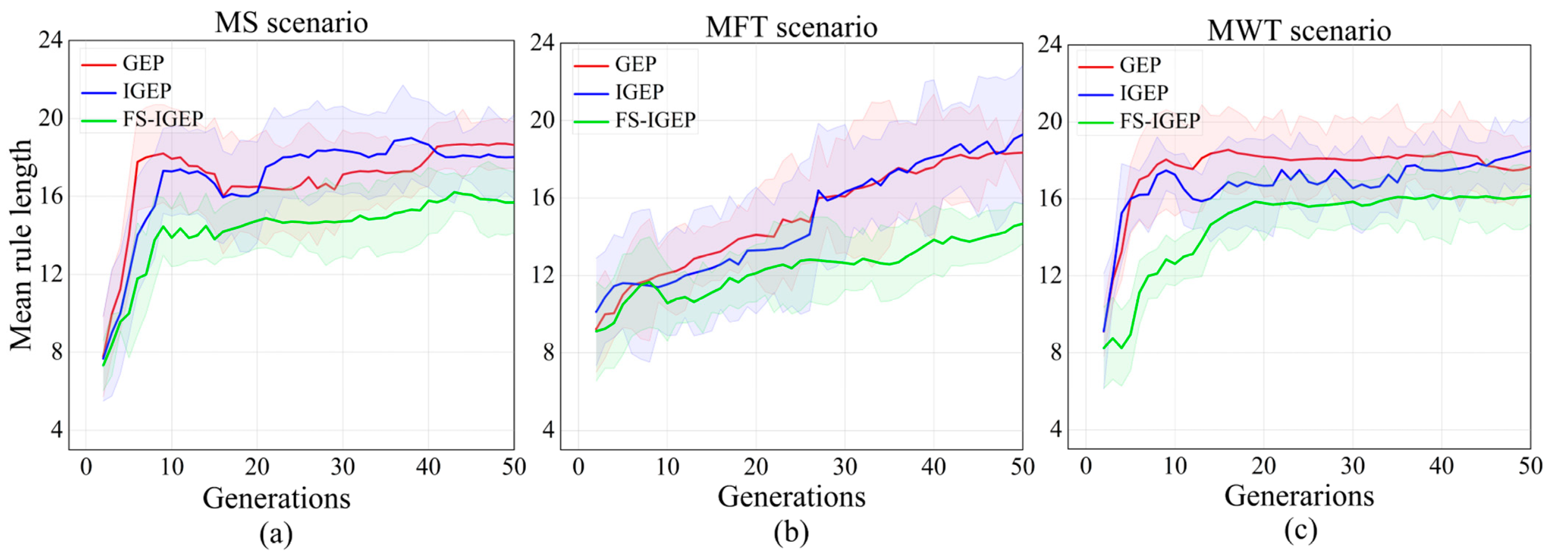
In scheduling processes, it is crucial to provide concise, simply interpretable dispatching rules. Rule size, often described as the sum of all nodes included inside a rule, is an essential aspect that affects interpretability. The advantages of compact dispatching rules include a reduced computational complexity and greater generality. This paper employed the numerical reduction technique, as proposed by Mei [18], to simplify the rules and enhance our understanding of their complexity and interpretability. The changes in the mean rule size across generations for the MT, MWT, and MFT scenarios are illustrated in Figure 4a–c, respectively. The observation of Figure 5 indicates that, in all scenarios, the IGEP and GEP algorithms exhibited a tendency to generate rules of significantly larger size than those produced with the FS-IGEP algorithm. As we expected, the designed rule length of the FS-IGEP was significantly different from those generated with IGEP and GEP algorithms. This was because more compact feature sets can help GEP to obtain simpler and shorter rules. In addition, we can observe that the rule length of the IGEP was not too much different from the GEP. This shows that despite the improvements, GEP was unable to generate simplified rules without a feature selection mechanism.

In order to further understand the impact of feature selection on the structure of dispatching rules, we compared and analyzed the structure of the best-evolved rules using GEP, IGEP, and FS-IGEP algorithms. Specifically, our study took the best dispatching rule (its objective value being 1213.25) achieved using the GEP algorithm, the best rule (its objective value being 1199.34) obtained using the IGEP algorithm, and the best rule designed using the FS-IGEP algorithm (its objective value being 1186.61) to be found in the MWT scenario <4, 15, 95%>. This was because the mean weighted tardiness in scenario <4, 15, 95%> was more difficult to optimize than other scenarios. We noted that the smaller the values calculated using the rules, the more priority the operation had.

For the GEP algorithm, in the examined run, the terminal set consisted of NOIQ, NOINQ, WIQ, MWT, PT, NPT, OWT, WKR, NOR, MRT, and W (i.e., eleven features). For the dispatching rules obtained using the IGEP algorithm, all the features in the terminal set were used. There were seven features (NOIQ, WINQ, NPT, PT, W, WKR and NOR) selected as terminal set. Fewer features were used by the FS-IGEP algorithm compared to IGEP and GEP. However, the evolved dispatching rules obtained using the FS-IGEP algorithm had better performance than that of IGEP and GEP.

According to the numerical reduction technique, the dispatching rule achieved using the FS-IGEP algorithm could be simplified, as shown in Equation (16). It is noted that for all the operations in the queue of a machine, the machine-related features, such as the workload of the current queue (WIQ), was the same for all operations. This means that it was not a vitally important feature. This dispatching rule preferred to select the operation with smaller processing times (PT) and larger weights (W). It is interesting that this dispatching rule preferred operation with smaller work remaining (WKR) based on the first section of $r_1$ while it tended to select the operation with larger WKR, based partially on the second section of $r_1$. This indicates that although we can interpret the rules to some extent, it is still hard to completely understand the behavior of rules. We will continue to work on this topic in the future.

The rules evolved using the IGEP and GEP algorithms can be simplified, as shown in Equations (17) and (18), respectively. It can be seen that the rule structure of both $r_2$ and $r_3$ was more complex than that of FS-IGEP, even after simplification. In addition, $r_1$ contained more of the meaningful building blocks, such as PT/W and WINQ/W, that have been established to yield favorable outcomes in the context of minimizing the mean weighted tardiness in DJSS.

In general, the results of the analysis performed on the FS-IGEP evolved rules showed that the selection of important terminals led to a reduction in the length of the rules and a more concise structure. This, in turn, enhanced the interpretability of the dispatching rules and facilitated their application in practical production scenarios by decision makers.

$$r_1=\frac{\max \left(PT,NPT\right)+WKR}{W}+\max \left(\frac{PT}{W},\frac{WINQ}{W}+NOR+WKR\right)$$

(16)

$$\begin{array}{l}{r}_2=(WIQ+NPT+FDD)\times \frac{NOR}{W}+\max (AT,PT\times NPT)\\ +NOPS+2DD\times \min (\frac{S{L}^2}{NOR+PT})-MRT\end{array}$$

(17)

$$\begin{array}{l}{r}_3=\frac{NOIQ+MRT}{W}-\left(W\times NOR-\max \left(\frac{NOIQ+MRT}{W}\right)\right)\\ -\min \left(\left(NOIQ,FDD\right)+\left(PT+NOINQ\right)\right)\\ +ORT\times \frac{WKR}{W^2}-WIQ\end{array}$$

(18)

5.1.3. Efficiency

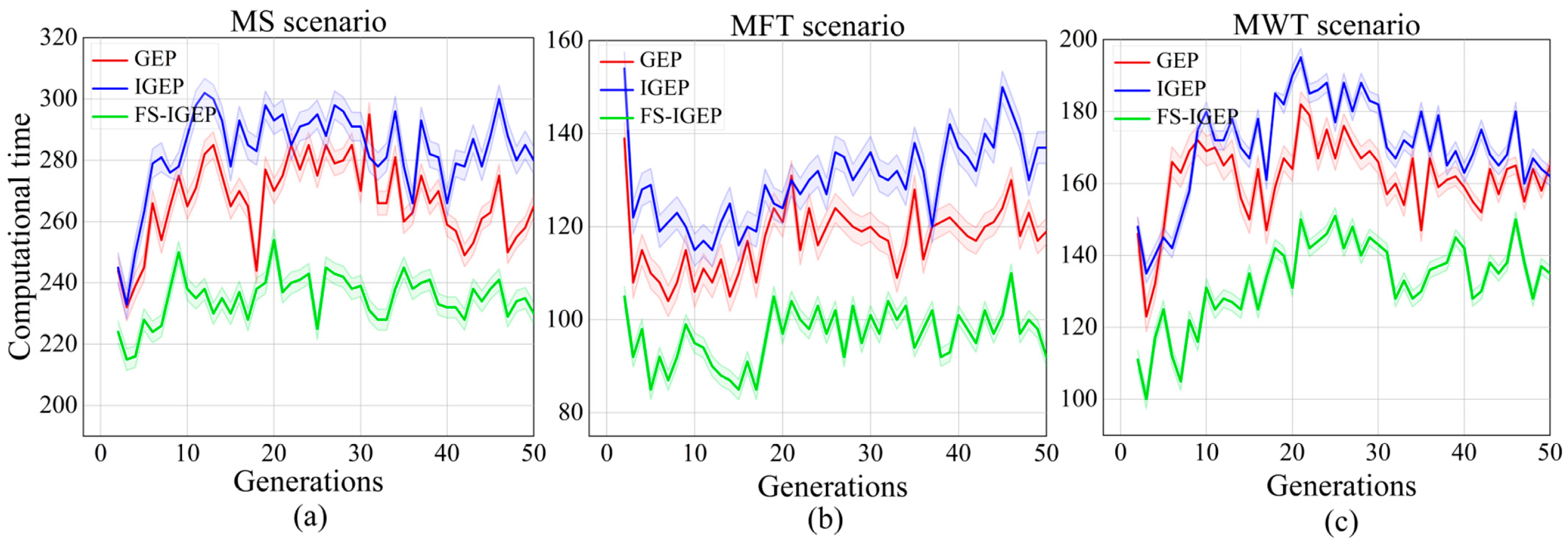
Given that enhancing the efficacy of the GEP algorithm through the utilization of feature selection was a primary objective of this study, it is imperative to conduct an analysis of the computational time. Figure 5a–c shows the computational time of 30 independent runs on the training set across generations in the MS, MFT, MWT scenario, respectively. The simulation results show that the computational budget of the FS-IGEP algorithm was significantly less than that of the IGEP and GEP algorithms in all mentioned scenarios. This is consistent with our expectation that the rules designed with a limited terminal set with chosen features were relatively short and simple, which reduced the time for fitness evaluation and improved the efficiency of the algorithm. Moreover, it was observed that the IGEP algorithm had higher computational complexity and more computational time than the GEP algorithm in the three scenarios. These observations offered valuable insights regarding the function of VNS. While the VNS algorithm could help GEP to find more competitive rules through the variable neighborhood search, it did not help GEP to reduce the computational budget. This further confirmed the role of feature selection in generating compact and understandable dispatching rules in a feasible computational time.

Figure 5. The computational time of the GEP algorithms in the three scenarios: (a) computational time across generations in the MS scenario; (b) computational time across generations in the MFT scenario; (c) computational time across generations in the MWT scenario.

Figure 5. The computational time of the GEP algorithms in the three scenarios: (a) computational time across generations in the MS scenario; (b) computational time across generations in the MFT scenario; (c) computational time across generations in the MWT scenario.

5.2. Feature Selection

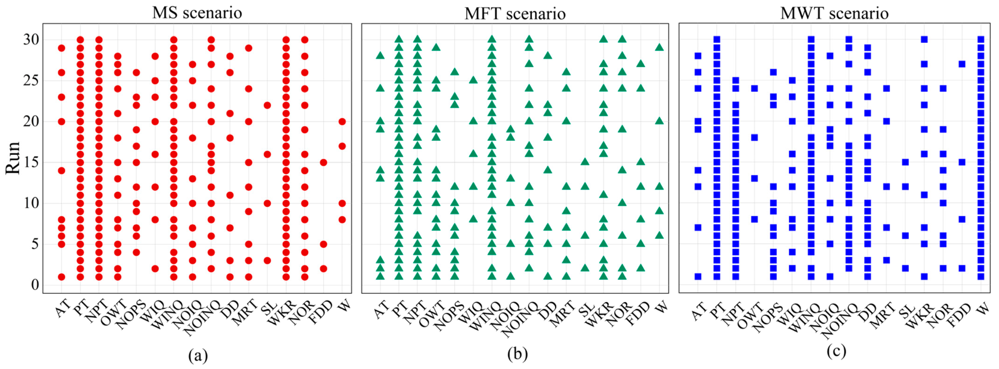
The contribution of each feature to the three scheduling objectives has been analyzed and a subset of the features that play an important role in designing dispatching rules in the three dynamic job-shop scenarios have been selected in this section. The results of the feature selection process for the MT, MWT, and MFT scenarios are presented in Figure 6a–c, respectively. These figures depict the outcomes of 30 independent runs of the proposed algorithm. Each column of a matrix represents a feature, whereas each row represents a run (for specifics, see Table 1). A point is drawn at the intersection of the selected feature $f$ and the $i$th run.

For the MS scenario, the feature PT, NPT, and WKR were selected in all 30 runs. This indicates that the processing time of operations in the MS scenario had an important impact on the computation of job priorities. At the same time, the machine prefers to select jobs with shorter processing times, fewer remaining processes, and small residual workloads, which is in line with the logic of shortening the makespan. Moreover, the features NOINQ, NOR, and OWT were selected in more than half of the running times of the algorithm, indicating that they significantly contributed to the generation of optimal dispatching rules at least half of the time. It can also be seen that the feature FDD, W, and SL were selected only a few times, which indicated that these features were irrelevant or redundant in this scenario and may not have contributed to the generation of best dispatching rules. The significance of the remaining features, namely AT, NOPS, WIQ, NOIQ, DD, and MRT, is not distinctly evident.

Regarding the MFT scenario, the feature PT was selected in all 30 runs. This indicates that, as in the MS scenario, the processing time of the operation also had a significant impact on the computation of job priorities in the MFT scenario. In addition, the machine preferentially selected jobs with short processing times, which can shorten the flow time of the jobs as much as possible. WINQ and NPT were selected only a few times more than PT, which means that the jobs with fewer workloads in the next operation had a higher priority to be processed. NOINQ and WKR were also selected in more than half of the runs, indicating that machines in the MFT scenario preferred to select the jobs with fewer remaining workloads and fewer operations in the next waiting queue. To put it simply, the characteristics of the next operation were the key point to designing effective dispatching rules in the MFT scenario. This lack of selection of the WIQ, NOIQ, SL, and W features over most runs implies that they did not contribute to the best-developed rules for the MFT objective. However, the contribution of AT, OWT, NOPS, DD, MRT, NOR, and FDD to the MFT scenario is not very clear.

In terms of the MWT scenario, PT and W were selected in the whole running process of the algorithm, which indicates that the machine preferred to prioritize the jobs with short processing time and high weight, so as to shorten the tardiness. This is consistent with the general conclusion in the field of production scheduling that PT and W were important features influencing the mean weighted tardiness. In addition to the aforementioned features, it was observed that WIQN, NOINQ, and NPT were commonly selected over a large number of iterations, indicating the significance of the workload data in the subsequent queues toward the minimization of the MWT objective. Unlike the findings of early research [60], the inclusion of terminal DD in the feature sets was not deemed irrelevant, as it was selected over 60% of the time. The observed phenomenon could potentially be related to the experimental setup, which incorporated three distinct categories of due date constraints, namely light, medium, and tight. MRT, OWT, FDD, and SL were selected less frequently, indicating that these features may have been redundant or irrelevant in the MWT scenario. In addition, the significance of the remaining features is unclear.

Figure 6. The matrix plot of the feature selection results of the proposed algorithm in the three scenarios: (a) selected features using the FS-IGEP algorithm for the MS scenario; (b) selected features using the FS-IGEP algorithm for the MFT scenario; (c) selected features using the FS-IGEP algorithm for the MWT scenario.

Figure 6. The matrix plot of the feature selection results of the proposed algorithm in the three scenarios: (a) selected features using the FS-IGEP algorithm for the MS scenario; (b) selected features using the FS-IGEP algorithm for the MFT scenario; (c) selected features using the FS-IGEP algorithm for the MWT scenario.

In summary, the following observations can be derived from the experimental results:

(1) The majority of the candidate features exhibited no relevance to the optimal dispatching rules across all three aforementioned scenarios.

(2) The relevance of features was dependent on the job-shop scenario and the optimization objective. For example, the WKR held significant importance as a terminal in the MS and MFT scenarios, whereas its relevance was comparatively low or insignificant in the MWT scenario.

(3) There were still some essential features, such as PT and WINQ, that were crucial for all evaluated situations.

Table 7 summarizes the selected key features for the three dynamic job-shop scenarios mentioned above.

Table 7. The key feature set for the three dynamic job-shop scenarios.

Scenario	Key Feature Set
MS scenario	PT, NPT, WINQ, WKR, NOINQ, NOR, OWT
MFT scenario	PT, NPT, WINQ, WKR, NOINQ
MWT scenario	PT, W, WINQ, NOINQ, NPT, DD

Table 7. The key feature set for the three dynamic job-shop scenarios.

Scenario	Key Feature Set
MS scenario	PT, NPT, WINQ, WKR, NOINQ, NOR, OWT
MFT scenario	PT, NPT, WINQ, WKR, NOINQ
MWT scenario	PT, W, WINQ, NOINQ, NPT, DD

6. Conclusions

In this paper, in order to increase the convergence speed of the evolutionary algorithm and to improve rule understandability while using fewer features, we proposed a feature selection mechanism to design dispatching rules for the DJSS with improved gene expression programming (IGEP). An improved GEP approach, employing an adaptive variable neighborhood search method, was developed to search for competitive dispatching rules in a large heuristic search space for different scheduling scenarios. Based on the optimal rules obtained using the IGEP algorithm, and considering the fitness of the rules and feature contribution to the rules, the subset of features that played an important role in mining dispatching rules were selected from the original terminal set using a weighted voting ranking method. Finally, based on the evolutionary information from the improved GEP and selected features, the proposed approach successfully achieved effective and interpretable rules for DJSS. The proposed algorithm (FS-IGEP) was compared to two algorithms (GEP, IGEP) in an MS scenario, MFT scenario, and MWT scenario, with respect rule performance, rule length, and efficiency.

The experimentally obtained results demonstrated the effectiveness of the proposed approach for designing more effective and interpretable rules while reducing computational time considerably. Considering the distribution of features in the best-evolved rules, the FS-IGEP algorithm obtained compact rules with a smaller selected terminal. Based on the rule analysis, it was revealed that the FS-IGEP had the ability to find more building blocks for improving the rule quality. In addition to the compact structure, the FS-IGEP rules presented overall improvement in the three considered scenarios, compared to the other rules designed using other two algorithms (GEP, IGEP).

When working with complex production systems and a large number of features from jobs and machines, feature selection becomes a crucial task in the automated design of dispatching rules. More research ought to be conducted in the future, to increase the accuracy of the feature selection. The feature selection mechanism will also receive more attention in our feature studies so that we can better grasp when to use it and how to improve its effectiveness. It will be necessary to use various standard scheduling issues to demonstrate the significance of feature selection. In contrast to previous simple local search algorithms employed for the purpose of facilitating GEP, the suggested adaptive variable neighborhood search exhibited favorable characteristics for both exploration and exploitation. Therefore, it was not easily trapped at the local optima. Subsequent studies may delve deeper into the behavior of the heuristic with the goal of reducing the number of necessary parameters and enhancing its adaptability.

References

1. Liu, Y.; Jin, S.; Zhou, J.; Hu, Q. A branch-and-bound algorithm for the unit-capacity resource constrained project scheduling problem with transfer times. Comput. Oper. Res. 2023, 151, 106097. [Google Scholar] [CrossRef]
2. Liu, H.; Wang, Y.; Lee, L.H.; Chew, E.P. An approximate dynamic programming approach for production-delivery scheduling under non-stationary demand. Nav. Res. Logist. 2022, 69, 511–528. [Google Scholar] [CrossRef]
3. Xue, Y.; Wang, Y.; Liang, J. A self-adaptive gradient descent search algorithm for fully-connected neural networks. Neurocomputing 2022, 478, 70–80. [Google Scholar] [CrossRef]
4. Marichelvam, M.K.; Geetha, M.; Tosun, Ö. An improved particle swarm optimization algorithm to solve hybrid flowshop scheduling problems with the effect of human factors—A case study. Comput. Oper. Res. 2020, 114, 104812. [Google Scholar] [CrossRef]
5. Behnamian, J.; Memar Dezfooli, S.; Asgari, H. A scatter search algorithm with a novel solution representation for flexible open shop scheduling: A multi-objective optimization. J. Supercomput. 2021, 77, 13115–13138. [Google Scholar] [CrossRef]
6. Lin, S.W.; Cheng, C.Y.; Pourhejazy, P.; Ying, K.C. Multi-temperature simulated annealing for optimizing mixed-blocking permutation flowshop scheduling problems. Expert Syst. Appl. 2021, 165, 113837. [Google Scholar] [CrossRef]
7. Chen, R.; Yang, B.; Li, S.; Wang, S. A self-learning genetic algorithm based on reinforcement learning for flexible job-shop scheduling problem. Comput. Ind. Eng. 2020, 149, 106778. [Google Scholar] [CrossRef]
8. ROSELINE, J.V.; SARAVANAN, D. Ant Colony Optimization Used in Backward Production Scheduling-Single Stage Process. J. Algebr. Stat. 2022, 13, 1090–1100. [Google Scholar]
9. Shady, S.; Kaihara, T.; Fujii, N.; Kokuryo, D. Automatic design of dispatching rules with genetic programming for dynamic job shop scheduling. IFIP Adv. Inf. Commun. Technol. 2020, 591, 399–407. [Google Scholar]
10. Braune, R.; Benda, F.; Doerner, K.F.; Hartl, R.F. A genetic programming learning approach to generate dispatching rules for flexible shop scheduling problems. Int. J. Prod. Econ. 2022, 243, 108342. [Google Scholar] [CrossRef]
11. Jemmali, M.; Ben Hmida, A. Quick dispatching-rules-based solution for the two parallel machines problem under mold constraints. Flex Serv. Manuf. J. 2023, 1–26. [Google Scholar] [CrossRef]
12. Zhuang, Z.; Li, Y.; Sun, Y.; Qin, W.; Sun, Z.H. Network-based dynamic dispatching rule generation mechanism for real-time production scheduling problems with dynamic job arrivals. Robot. Comput. Integr. Manuf. 2022, 73, 102261. [Google Scholar] [CrossRef]
13. Gohareh, M.M.; Mansouri, E. A simulation-optimization framework for generating dynamic dispatching rules for stochastic job shop with earliness and tardiness penalties. Comput. Oper. Res. 2022, 140, 105650. [Google Scholar] [CrossRef]
14. Nguyen, S.; Mei, Y.; Xue, B.; Zhang, M. A hybrid genetic programming algorithm for automated design of dispatching rules. Evol. Comput. 2019, 27, 467–496. [Google Scholar] [CrossRef] [PubMed]
15. Burke, E.K.; Gendreau, M.; Hyde, M.; Kendall, G.; Ochoa, G.; Özcan, E.; Qu, R. Hyper-heuristics: A survey of the state of the art. J. Oper. Res. Soc. 2013, 64, 1695–1724. [Google Scholar] [CrossRef]
16. Zhang, H.; Qin, C.; Zhang, W.; Xu, Z.; Xu, G.; Gao, Z. Energy-saving scheduling for flexible job shop problem with AGV transportation considering emergencies. Systems 2023, 11, 103. [Google Scholar] [CrossRef]
17. Zhao, J.; Cao, B.; Liu, X.; Yang, P.; Singh, A.K.; Lv, Z. Multiobjective Multiple Mobile Sink Scheduling via Evolutionary Fuzzy Rough Neural Network for Wireless Sensor Networks. IEEE Trans. Fuzzy Syst. 2022, 30, 4630–4641. [Google Scholar] [CrossRef]
18. Mei, Y.; Zhang, M.; Nyugen, S. Feature selection in evolving job shop dispatching rules with genetic programming. In Proceedings of the Genetic and Evolutionary Computation Conference, Denver, CO, USA, 20–24 July 2016; pp. 365–372. [Google Scholar]
19. Zeiträg, Y.; Figueira, J.R.; Horta, N.; Neves, R. Surrogate-assisted automatic evolving of dispatching rules for multi-objective dynamic job shop scheduling using genetic programming. Expert Syst. Appl. 2022, 209, 118194. [Google Scholar] [CrossRef]
20. Rafsanjani, M.K.; Riyahi, M. A new hybrid genetic algorithm for job shop scheduling problem. Int. J. Adv. Intell. Paradig. 2020, 16, 157–171. [Google Scholar] [CrossRef]
21. Lee, J.; Perkins, D. A simulated annealing algorithm with a dual perturbation method for clustering. Pattern Recognit. 2021, 112, 107713. [Google Scholar] [CrossRef]
22. Yi, N.; Xu, J.; Yan, L.; Huang, L. Task optimization and scheduling of distributed cyber–physical system based on improved ant colony algorithm. Future Gener. Comput. Syst. 2020, 109, 134–148. [Google Scholar] [CrossRef]
23. Shady, S.; Kaihara, T.; Fujii, N.; Kokuryo, D. A hyper-heuristic framework using GP for dynamic job shop scheduling problem. In Proceedings of the 64th Annual Conference of the Institute of Systems, Control and Information Engineers, New Orleans, LA, USA, 30 May–2 June 2020; pp. 248–252. [Google Scholar]
24. Liu, L.; Shi, L. Automatic Design of Efficient Heuristics for Two-Stage Hybrid Flow Shop Scheduling. Symmetry 2022, 14, 632. [Google Scholar] [CrossRef]
25. Burke, E.K.; Hyde, M.R.; Kendall, G.; Woodward, J. Automating the packing heuristic design process with genetic programming. Evol. Comput. 2012, 20, 63–89. [Google Scholar] [CrossRef] [PubMed]
26. Kieffer, E.; Danoy, G.; Brust, M.R.; Bouvry, P.; Nagih, A. Tackling large-scale and combinatorial bi-level problems with a genetic programming hyper-heuristic. IEEE Trans. Evolut. Comput. 2019, 24, 44–56. [Google Scholar] [CrossRef]
27. Tan, B.; Ma, H.; Mei, Y.; Zhang, M. A cooperative coevolution genetic programming hyper-heuristics approach for on-line resource allocation in container-based clouds. IEEE Trans. Evolut. Comput. 2020, 10, 1500–1514. [Google Scholar] [CrossRef]
28. Gulić, M.; Jakobović, D. Evolution of vehicle routing problem heuristics with genetic programming. In Proceedings of the 2013 36th International Convention on Information and Communication Technology, Electronics and Microelectronics (MIPRO), Opatija, Croatia, 20–24 May 2013; pp. 988–992. [Google Scholar]
29. Jacobsen-Grocott, J.; Mei, Y.; Chen, G.; Zhang, M. Evolving heuristics for dynamic vehicle routing with time windows using genetic programming. In Proceedings of the 2017 IEEE Congress on Evolutionary Computation (CEC), Donostia-San Sebastián, Spain, 5–8 June 2017; pp. 1948–1955. [Google Scholar]
30. Branke, J.; Hildebrandt, T.; Scholz-Reiter, B. Hyper-heuristic evolution of dispatching rules: A comparison of rule representations. Evol. Comput. 2015, 23, 249–277. [Google Scholar] [CrossRef]
31. Balusamy, J.; Karunakaran, M. Hybridization of immune with particle swarm optimization in task scheduling on smart devices. Distrib. Parallel Databases 2022, 40, 85–107. [Google Scholar] [CrossRef]
32. Ferreira, C.; Figueira, G.; Amorim, P. Effective and interpretable dispatching rules for dynamic job shops via guided empirical learning. Omega 2022, 111, 102643. [Google Scholar] [CrossRef]
33. Nie, L.; Shao, X.; Gao, L.; Li, W. Evolving scheduling rules with gene expression programming for dynamic single-machine scheduling problems. Int. J. Adv. Manuf. Technol. 2010, 50, 729–747. [Google Scholar] [CrossRef]
34. Nie, L.; Gao, L.; Li, P.; Shao, X. Reactive scheduling in a job shop where jobs arrive over time. Comput. Ind. Eng. 2013, 66, 389–405. [Google Scholar] [CrossRef]
35. Ozturk, G.; Bahadir, O.; Teymourifar, A. Extracting priority rules for dynamic multi-objective flexible job shop scheduling problems using gene expression programming. Int. J. Prod. Res. 2019, 57, 3121–3137. [Google Scholar] [CrossRef]
36. Teymourifar, A.; Ozturk, G.; Ozturk, Z.K.; Bahadir, O. Extracting new dispatching rules for multi-objective dynamic flexible job shop scheduling with limited buffer spaces. Cognit. Comput. 2020, 12, 195–205. [Google Scholar] [CrossRef]
37. Zhang, C.; Zhou, Y.; Peng, K.; Li, X.; Lian, K.; Zhang, S. Dynamic flexible job shop scheduling method based on improved gene expression programming. Meas. Control 2021, 54, 1136–1146. [Google Scholar] [CrossRef]
38. Friedlander, A.; Neshatian, K.; Zhang, M. Meta-learning and feature ranking using genetic programming for classification: Variable terminal weighting. In Proceedings of the 2011 IEEE Congress of Evolutionary Computation (CEC), New Orleans, LA, USA, 5–8 June 2011; pp. 941–948. [Google Scholar]
39. Mei, Y.; Nguyen, S.; Xue, B.; Zhang, M. An Efficient Feature Selection Algorithm for Evolving Job Shop Scheduling Rules with Genetic Programming. IEEE Trans. Emerg. Top. Comput. Intell. 2017, 1, 339–353. [Google Scholar] [CrossRef]
40. Shady, S.; Kaihara, T.; Fujii, N.; Kokuryo, D. A novel feature selection for evolving compact dispatching rules using genetic programming for dynamic job shop scheduling. Int. J. Prod. Res. 2022, 60, 4025–4048. [Google Scholar] [CrossRef]
41. Shady, S.; Kaihara, T.; Fujii, N.; Kokuryo, D. Feature selection approach for evolving reactive scheduling policies for dynamic job shop scheduling problem using gene expression programming. Int. J. Prod. Res. 2022, 1–24. [Google Scholar] [CrossRef]
42. Panda, S.; Mei, Y.; Zhang, M. Simplifying Dispatching Rules in Genetic Programming for Dynamic Job Shop Scheduling. In European Conference on Evolutionary Computation in Combinatorial Optimization; Springer International Publishing: Cham, Switzerland, 2022; pp. 95–110. [Google Scholar]
43. Huang, Z.; Zhang, F.; Mei, Y.; Zhang, M. An Investigation of Multitask Linear Genetic Programming for Dynamic Job Shop Scheduling. In European Conference on Genetic Programming (Part of EvoStar); Springer: Cham, Switzerland, 2022; pp. 162–178. [Google Scholar]
44. Fan, H.; Xiong, H.; Goh, M. Genetic programming-based hyper-heuristic approach for solving dynamic job shop scheduling problem with extended technical precedence constraints. Comput. Oper. Res. 2021, 134, 105401. [Google Scholar] [CrossRef]
45. Wagner, S.; Mönch, L. A variable neighborhood search approach to solve the order batching problem with heterogeneous pick devices. Eur. J. Oper. Res. 2023, 304, 461–475. [Google Scholar] [CrossRef]
46. Shao, W.; Shao, Z.; Pi, D. Multi-local search-based general variable neighborhood search for distributed flow shop scheduling in heterogeneous multi-factories. Appl. Soft. Comput. 2022, 125, 109138. [Google Scholar] [CrossRef]
47. Lei, D.; Chen, X. An improved variable neighborhood search for parallel drone scheduling traveling salesman problem. Appl. Soft Comput. 2022, 127, 109416. [Google Scholar] [CrossRef]
48. Zhang, F.; Mei, Y.; Nguyen, S.; Zhang, M. Evolving scheduling heuristics via genetic programming with feature selection in dynamic flexible job-shop scheduling. IEEE Trans. Cybern. 2020, 51, 1797–1811. [Google Scholar] [CrossRef]
49. Park, J.; Mei, Y.; Nguyen, S.; Chen, G.; Zhang, M. An investigation of ensemble combination schemes for genetic programming based hyper-heuristic approaches to dynamic job shop scheduling. Appl. Soft. Comput. 2018, 63, 72–86. [Google Scholar] [CrossRef]
50. Ari, D.; Alagoz, B.B. A differential evolutionary chromosomal gene expression programming technique for electronic nose applications. Appl. Soft. Comput. 2023, 136, 110093. [Google Scholar] [CrossRef]
51. Cao, B.; Zhao, J.; Liu, X.; Arabas, J.; Tanveer, M.; Singh, A.K.; Lv, Z. Multiobjective evolution of the explainable fuzzy rough neural network with gene expression programming. IEEE Trans. Fuzzy Syst. 2022, 30, 4190–4200. [Google Scholar] [CrossRef]
52. Saxena, R.; Arora, D.; Nagar, V. Efficient blockchain addresses classification through cascading ensemble learning approach. Int. J. Electron. Secur. 2023, 15, 195–210. [Google Scholar] [CrossRef]
53. Campagner, A.; Ciucci, D.; Cabitza, F. Aggregation models in ensemble learning: A large-scale comparison. Inf. Fusion 2023, 90, 241–252. [Google Scholar] [CrossRef]
54. Holthaus, O. Scheduling in job shops with machine breakdowns: An experimental study. Comput. Ind. Eng. 1999, 36, 137–162. [Google Scholar] [CrossRef]
55. Zhang, G.; Lu, X.; Liu, X.; Zhang, L.; Wei, S.; Zhang, W. An effective two-stage algorithm based on convolutional neural network for the bi-objective flexible job shop scheduling problem with machine breakdown. Expert Syst. Appl. 2022, 203, 117460. [Google Scholar] [CrossRef]
56. Geurtsen, M.; Didden, J.B.; Adan, J.; Atan, Z.; Adan, I. Production, maintenance and resource scheduling: A review. Eur. J. Oper. Res. 2022, 305, 501–529. [Google Scholar] [CrossRef]
57. Xiong, H.; Shi, S.; Ren, D.; Hu, J. A survey of job shop scheduling problem: The types and models. Comput. Oper. Res. 2022, 142, 105731. [Google Scholar] [CrossRef]
58. Xu, K.; Liu, Y.; Tang, R.; Zuo, J.; Zhu, J.; Tang, C. A novel method for real parameter optimization based on gene expression programming. Appl. Soft Comput. 2009, 9, 725–737. [Google Scholar] [CrossRef]
59. Zhang, L.; Tang, Q.; Wu, Z.; Wang, F. Mathematical modeling and evolutionary generation of rule sets for energy-efficient flexible job shops. Energy 2017, 138, 210–227. [Google Scholar] [CrossRef]
60. Ghasemi, A.; Ashoori, A.; Heavey, C. Evolutionary learning based simulation optimization for stochastic job shop scheduling problems. Appl. Soft Comput. 2021, 106, 107309. [Google Scholar] [CrossRef]
Figure 1. The framework of the proposed approach.
Applsci 13 06631 g001
Figure 2. The flow chart of the IGEP algorithm.
Applsci 13 06631 g002
Figure 3. Genotype–phenotype of a dispatching rule, encoded as an expression tree.
Applsci 13 06631 g003
Figure 4. The mean rule size of the GEP algorithms in the three scenarios: (a) mean rule size across generations in the MS scenario; (b) mean rule size across generations in the MFT scenario; (c) mean rule size across generations in the MWT scenario.
Applsci 13 06631 g004