Article

A Jacobian-Free Newton–Krylov Method to Solve Tumor Growth Problems with Effective Preconditioning Strategies

Department of Mathematical Engineering, Istanbul Technical University, Maslak, Istanbul 34667, Turkey
*
Author to whom correspondence should be addressed.
Appl. Sci. 2023, 13(11), 6579; https://doi.org/10.3390/app13116579
Submission received: 4 March 2023 / Revised: 13 April 2023 / Accepted: 24 April 2023 / Published: 29 May 2023
(This article belongs to the Section Applied Physics General)

Abstract

:
A Jacobian-free Newton–Krylov (JFNK) method with effective preconditioning strategies is introduced to solve a diffusion-based tumor growth model, also known as the Fisher–Kolmogorov partial differential equation (PDE). The time discretization of the PDE is based on the backward Euler and the Crank–Nicolson methods. Second-order centered finite differencing is used for the spatial derivatives. We introduce two physics-based preconditioners associated with the first- and second-order temporal discretizations. The theoretical time and spatial accuracies of the numerical scheme are verified through convergence tables and graphs that correspond to different computational settings. We present efficiency studies with and without using the preconditioners. Our numerical findings indicate the excellent performance of the newly proposed preconditioning strategies. In other words, when we turn the preconditioners on, the average number of GMRES and the Newton iterations are significantly reduced.

1. Introduction

Gliomas are the most common and very aggressive type of brain tumor. They have been known to be incurable due to their large invasion capacity. It is important to have good mathematical models and their numerical solutions to understand the true nature and the underlying physical mechanism of this phenomenon. Over the years, researchers have paid a lot of attention to the modeling part and solution techniques. A set of several review articles on this topic can be found in the following references [1,2,3,4,5]. Widely used mathematical models are based on the nonlinear reaction–diffusion type partial differential equations (PDEs) to describe the time evolution of the tumor growth. It is difficult to solve these models analytically because of the existence of nonlinearity and discontinuity in the source and diffusion coefficient terms. On the other hand, numerical solutions and computer simulations have been good alternatives. In the last two decades, there have been several attempts such as variational iteration method (VIM) [6], stochastic models [7,8], finite element methods (FEM) [9,10,11,12], finite difference schemes (FDSs) [6,11,13,14], cubic B-spline collocation methods [12], hybrid models [7,10], and Bayesian approaches [15] to approximately solve the mathematical model and simulate the time behavior of the tumor concentrations in the glioma cells.
In 2015, Wu et al. [6] introduced a variational iteration method (VIM) to study this problem by transforming the reaction–diffusion equation into an equivalent integral equation. This method enables one to avoid the treatment of the time derivatives as in classical finite difference sense. However, the method involves the so-called Picard iteration procedure that can be computationally very inefficient.
Later on, Mach et al. [9] investigated the finite-element nonlinear Galerkin method (FEM) in one spatial dimension and its application to the selected reaction–diffusion systems. Another FEM approach was carried out by Dehghan and Narimani [16] in 2018 and called the element-free Galerkin method to simulate the effects of cancer cell invasion on the surrounding tissue. We note that even though the FEM is preferable for irregular geometries compared to the FDS, the FEM is more prone to stability issues especially when the discontinuous diffusion coefficients and sharp gradients exist in the system.
In 2020, Dehghan and Narimani [17] used a collocation meshless technique called the radial basis function-generated finite difference (RBF-FD) scheme to solve the reaction–diffusion model in multi-dimensional settings. They employed a first-order semi-implicit scheme to approximate the time variable and solved the resulting linear system of algebraic equations using the biconjugate gradient stabilized (BiCGSTAB) iterative scheme with a zero-fill incomplete lower–upper (ILU) preconditioner. An obvious drawback of this approach is that, despite being incomplete, it involves an expensive LU decomposition, let alone the positive-definite requirement of the CG method.
Another study was carried out by Kapoor and Joshi in [12]. They used a modified cubic uniform algebraic hyperbolic tension B-spline differential quadrature method to discretize the spatial partial derivatives in 1D and 2D reaction–diffusion systems. They utilized a strong stability preserving Runge–Kutta (SSP-RK4) time scheme to solve the resulting ordinary differential Equation (ODE). One disadvantage of this approach is that it can be expensive to implement due to the high number of function evaluations in the cubic spline procedure and due to the stability restrictions imposed by the explicit SSP-RK4 method.
In this study, we adopt the proliferation–invasion (PI) model that is assumed to capture the most fundamental features of cancer cells (e.g., cell growth cannot be restrained and can occupy surrounding tissues). In this model, the rate of change of cell density can be written as a sum of the invasion of cells into nearby tissue (heterogeneous diffusion coefficient times the cell density) and the proliferation of cells (in terms of logistic growth). The resulting equations are similar to the reaction–diffusion equation with radiotherapy and chemotherapy effects [18]. We note that we neglect the effects of radiotherapy and chemotherapy in this paper because, for the time being, we aim to introduce an accurate and effective solution methodology and test its convergence and efficiency on a simplified model. However, we will consider a more realistic model with all additional effects included in a follow-up study [17]. We also note that a one-dimensional simplified model was numerically studied by the co-author of this work in [19]. The major drawback of [19] is that it relies on the construction, storage, and inversion of the Jacobian matrix of the nonlinear system. This approach can be computationally very inefficient and very difficult to implement in a situation where discontinuous or solution-dependent diffusion coefficient exists together with nonlinear source terms, which is the case herein.
In this paper, we utilize a Jacobian-free Newton–Krylov (JFNK) method with new effective preconditioning strategies to solve the growth model. The JFNK methods are synergic combinations of Newton type-methods for the super linearly convergent solution of nonlinear equations and Krylov subspace methods for solving the linear equations [20]. The implementation of a JFNK method requires the solution of a linear system that comes from the Newton correction step. Generally, the linear system is solved based on a particular Krylov subspace method and the generalized minimal residual (GMRES) iterative method [20,21]. The main advantage of a Jacobian-free Newton–Krylov method is that it does not require the formation, storage, and inversion of the Jacobian matrix. Perhaps, this itself is the main reason why the JFNK methods became very popular in the scientific community. They have been successfully used to solve boundary or initial valued problems coming from diverse areas; compressible or incompressible fluid dynamics problems, heat transfer engineering and thermal hydraulic problems, neutronics applications, solid mechanics problems, astrophysical applications, and optimization problems from industry to name a few [20,22,23,24,25,26,27,28].
As part of the JFNK method, we need to include a preconditioning step to accelerate the convergence of the Krylov block. We note that the preconditioning step became almost standard for any type of iterative scheme [21,29,30]. Here, we introduce very effective preconditioning techniques that share similarities to those presented in [31,32,33,34,35] in such a way that they all rely on the underlying physics. In the literature, these kinds of methods are referred to as physics-based or physical preconditioning. The main benefit of this preconditioning strategy is that one can target a particular part of the model that creates stiffness or causes slow convergence and only apply the procedure to such a part rather than to the entire system. The numerical results in Section 4 indicate that the new preconditioners perform very well, decreasing the average number of GMRES and the Newton iterations to very low numbers.
The organization of this paper is as follows: In Section 2, we define the governing equations. In Section 3, we describe the Jacobian-free Newton–Krylov (JFNK) method together with the new physics-based preconditioning techniques. In Section 4, we present our numerical results to verify the numerical convergence of the proposed schemes and to show the performance and capabilities of the new preconditioning strategies. In Section 5, we summarize our concluding remarks and hint at possible future works.

2. Governing Equations

The governing PDEs are based on the proliferation–invasion (PI) model [17,18,19,36] to describe glioma cell invasion throughout the brain as a reaction–diffusion process;
c ( x , y , t ) t = x D c ( x , y , t ) x + y D c ( x , y , t ) y + ρ c ( x , y , t ) 1 c ( x , y , t ) c max ,
where c ( x , y , t ) is the tumor concentration of glioma cells at spatial locations x , y and time t, ρ is the net proliferation rate in units d a y 1 , and D ( x , y ) is the diffusion coefficient. Notice that we can solve Equation (1) as a one- or two- dimensional model by simply turning the y derivatives off and on. The birth and death rates are included in ρ , assuming a Verhulst (logistic growth) law including a tissue-carrying capacity c max [37]. The diffusion coefficient can depend on the values of the concentration and may vary from patient to patient [38]. In this study, we use discontinuous diffusion coefficient profiles that contain low (gray region) and high (white region) diffusion zones [38]. In one- dimensional test cases, we use
D ( x ) = 0.13 if   0 x 7.5   ( gray   region ) 0.65 if   7.5 < x 42.5   ( white   region ) 0.13 if   42.5 < x 50   ( gray   region ) ,
where x belongs to the interval I = [ 0 , 50 ] , and in two -dimensional cases, as suggested by Shim et al. [39], we set
D ( x , y ) = 0.65 if   0 d 17.5   ( white   region ) 0.13 otherwise   ( gray   region ) ,
where d = ( x x 0 ) 2 + ( x y 0 ) 2 and ( x 0 y 0 ) = ( 25 , 25 ) is the center of the two-dimensional computational domain D = [ 0 , 50 ] × [ 0 , 50 ] . The zero-flux boundary conditions and one and two- dimensional Gaussian initial tumor profiles are defined as
c x ( 0 , y , t ) = c x ( 50 , y , t ) = c y ( x , 0 , t ) = c y ( x , 50 , t ) = 0 ,
c ( 0 , t ) = g ( x ) = 1 2 π ϵ e 1 2 x x 0 ϵ 2 c ( x , y , 0 ) = g ( x , y ) = 1 2 π ϵ e d 2 2 ϵ 2 ,
where we use ϵ = 0.01 in our calculations. Figure 1 illustrates one- and two- dimensional Gaussian initial tumors and discontinuous diffusion coefficient profiles.

3. Numerical Algorithm

We present two implicit time discretization methods: one is based on the first-order backward Euler and the other is the second-order Crank–Nicolson scheme. Here, we purposely considered two different time-convergent schemes. The first reason is the fact that the local time error can accumulate differently depending on the time accuracy of the method. Furthermore, the second reason is that the time accuracy can affect the overall performance of the JFNK method. In Section 4, we present a head on comparison study for the two time methods and the aforementioned numerically verified behaviors. The spatial derivatives are discretized using the second-order centered finite differencing procedure on a staggered grid configuration. An obvious advantage of using a staggered grid is that it enables us to position the discontinuous diffusion coefficients exactly at the cell edges, rather than extrapolating them from the cell centers.

3.1. The Backward Euler (BE) Method

The first-order backward Euler (BE) time scheme together with the second-order space discretization of Equation (1) can be given in the following form
c i , j n + 1 c i , j n Δ t D i + 1 2 , j c x i + 1 2 , j n + 1 D i 1 2 , j c x i 1 2 , j n + 1 Δ x D i , j + 1 2 c y i , j + 1 2 n + 1 D i , j 1 2 c y i , j 1 2 n + 1 Δ y ρ c i , j n + 1 1 c i , j n + 1 c max 0 ,
where c i , j n approximates the true solution at the grid location ( x i , y j ) and time t n (e.g., c i , j n c ( x i , y j , t n ) = c ( i Δ x , j Δ y , n Δ t ) and the following derivatives are approximated by
c x i + 1 2 , j n + 1 c i + 1 , j n + 1 c i , j n + 1 Δ x c x i 1 2 , j n + 1 c i , j n + 1 c i 1 , j n + 1 Δ x
c y i , j + 1 2 n + 1 c i , j + 1 n + 1 c i , j n + 1 Δ y , c y i , j 1 2 n + 1 c i , j n + 1 c i , j 1 n + 1 Δ y .
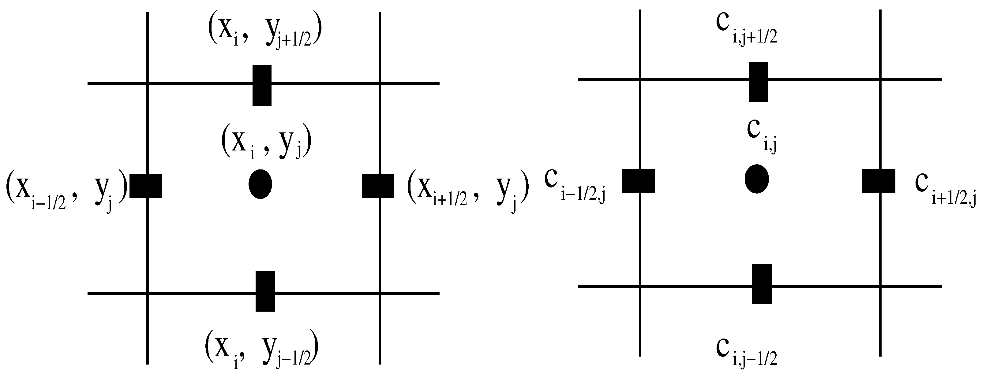
Here, Δ x = x i + 1 2 x i 1 2 and Δ y = y j + 1 2 y j 1 2 are the size of the ( i , j ) th cell in x and y directions, ( x i , y j ) represents the center of the ( i , j ) th cell, and ( x i ± 1 2 , y j ± 1 2 ) denote the left, right, top, and bottom edges of the ( i , j ) t h cell (Figure 2). The spatial domain [ 0 , 50 ] × [ 0 , 50 ] is divided into M x and M y sections in the x and y directions. We use the uniform grids in this study, implying that ( Δ x i , Δ y j ) = ( Δ x , Δ y ) = ( 50 M x , 50 M y ) where i = 0 , M x 1 and j = 0 , M y 1 .
We utilize the following discrete Neumann boundary conditions for Equation (4)
c x 1 2 , j n + 1 0 , c x M x 1 2 , j n + 1 0 , c y i , 1 2 n + 1 0 , c y i , M y 1 2 n + 1 0 .
Equation (7) can be used to set the ghost cell values in the x direction as
0 c x 1 2 , j n + 1 ( c 0 , j n + 1 c 1 , j n + 1 ) / Δ x c 1 , j n + 1 c 0 , j n + 1 ,
0 c x M x 1 2 , j n + 1 ( c M x , j n + 1 c M x 1 , j n + 1 ) / Δ x c M x , j n + 1 c M x 1 , j n + 1 ,
and, similarly, in the y direction as
0 c y i , 1 2 n + 1 ( c i , 0 n + 1 c i , 1 n + 1 ) / Δ y c i , 1 n + 1 c i , 0 n + 1 ,
0 c y i , M y 1 2 n + 1 ( c i , M y n + 1 c i , M y 1 n + 1 ) / Δ y c i , M y n + 1 c i , M y 1 n + 1 .

3.2. The Crank–Nicolson (CN) Method

The Crank–Nicolson method is a second-order accurate scheme in both time and space. It utilizes the time average of the flux and source terms together with the centered spatial discretizations. Along with these principles, the governing equation yields
c i , j n + 1 c i , j n Δ t 1 2 D i + 1 2 , j c x i + 1 2 , j n + 1 D i 1 2 , j c x i 1 2 , j n + 1 Δ x + D i + 1 2 , j c x i + 1 2 , j n D i 1 2 , j c x i 1 2 , j n Δ x 1 2 D i , j + 1 2 c y i , j + 1 2 n + 1 D i , j 1 2 c y i , j 1 2 n + 1 Δ y + D i , j + 1 2 c y , i , j + 1 2 n D i , j 1 2 c y i , j 1 2 n Δ y 1 2 ρ c i , j n + 1 1 c i , j n + 1 c max + ρ c i , j n 1 c i , j n c max 0 .
Equations (6) and (8) can be viewed as a system of nonlinear algebraic equations (e.g., F ( c ) 0 ) that need to be solved for the unknown c n + 1 . The resulting nonlinear equation system will be solved using the Jacobian-free Newton Krylov (JFNK) method [20,31,34]. After applying a desired number of nonlinear iterations, the JFNK method guarantees the convergence of all nonlinearities in the system. Of course, we have to keep in mind that, in order for the JFNK method—just like the other nonlinear solvers—to converge to a physically correct solution, we have to provide a good initial guess. This is not an issue here, because we are solving an initial value problem. In other words, at the beginning of each time update, we have a very good initial guess coming from the previous time step solution.

3.3. The Jacobian-Free Newton–Krylov Method

In the following section, we briefly describe the JFNK method. The JFNK method has two components, namely the Newton and Krylov blocks. The Newton block iteratively solves F ( c ) 0 over the sequence of a linear system defined by
J ( c k ) δ c k F ( c k ) , c k + 1 c k + δ c k , k = 0 , 1 ,
where J ( c k ) = F c is the Jacobian matrix and δ c k is the update vector. The Newton iteration is stopped if the following criterion is matched
F ( c k ) 2 < tol r e s F ( c 0 ) 2 ,
where tol r e s is the user-defined tolerance, typically 10 8 . The resulting linear system at the Newton correction step (Equation (9)) is solved utilizing a Krylov subspace method. In particular, we use the Arnoldi-based GMRES method [21]. At the beginning of the GMRES iteration, we need to define an initial residual, r 0 , for a given initial guess δ c 0 ,
r 0 F ( c ) J δ c 0 .
Since the Krylov (GMRES) iteration is executed at a fixed k, we omit the index k for convenience in Equation (11). Let j denote the Krylov iteration index. The jth Krylov iteration minimizes the quantity J δ c j + F ( c ) 2 within a subspace of small dimensions relative to n (the number of unknown vectors) in a least-squares sense. δ c j is drawn from the subspace spanned by the Krylov vectors, { r 0 , J r 0 , J 2 r 0 , , J j 1 r 0 } , and can be written as the following combination
δ c j δ c 0 + i = 0 j 1 β i ( J ) i r 0 ,
where the term β i minimizes the residual. We terminate the Krylov iteration using the following inexact Newton criteria [40]
J δ c j + F ( c ) 2 < γ F ( c ) 2 .
Here, parameter γ is chosen to determine the convergence of the linear solver at each Newton iteration (we usually set γ = 10 3 ). We note that one main advantage of the Krylov subspace method that we use here is that it does not need the formation of the Jacobian matrix. It only requires the matrix-vector multiplication, J v , where v { r 0 , J r 0 , J 2 r 0 , } . This is why it is simply referred to as the Jacobian-free implementation, in which the operation of the Jacobian matrix times a vector can be estimated by
J v F ( c + ϵ v ) F ( c ) ϵ ,
where ϵ = 1 n v 2 i = 1 n b | c i | + b , n is the dimension of the linear system, and b is a constant whose magnitude is within a few orders of magnitude of the square root of machine round-off (it is typically set to 10 6 for 64-bit double precision).
Remark 1.
We remark that we do not employ any global convergence strategy such as the trust region method or line search method to improve the convergence of the nonlinear block [21,41] in this research. Typically, the line search or trust region of globalization methods are employed if the initial guess is far from the solution or the converged solution is not physically the correct one. The main reason why we do not use such methods is that, in both methods, one needs to calculate the direction search vectors which require the knowledge of a Jacobian matrix (exact or approximate), but in our matrix’s free implementation, we do not calculate the Jacobian matrix by any means. The second reason is that we are solving an initial value problem and, at the beginning of each nonlinear iteration, the previous time step solutions become a very good initial guess for the next set of solutions. With regard to the second point, we also note that, despite the fact they are time implicit, our integration techniques do not use arbitrarily large time steps for accuracy reasons. Furthermore, this prevents us drifting far away from the next time level solutions.
As we pointed out earlier, we utilize preconditioning techniques to accelerate the convergence of the JFNK’s Krylov step. Usually, the original linear system (9) is modified when a preconditioner is in use (the Jacobian matrix is multiplied by a preconditioning matrix from the left or right). When the linear system is multiplied by a preconditioning matrix from the left, the resulting method is called the left preconditioner (or the right preconditioner if the multiplication is performed from the right). We note that the left preconditioner also modifies the right-hand side of the linear system (9), meaning that the modified nonlinear residuals must be recovered. This brings additional coding complexity and computational costs [20,21,42]. On the other hand, the right preconditioner does not affect the right-hand side term and does not possess the aforementioned difficulties. Therefore, we prefer the right preconditioning (RP) strategy in this paper.
The RP procedure modifies and improves the linear system (9) as follows
J P 1 ( P δ c ) F ( c ) ,
where P is the preconditioning matrix. The action of the right preconditioning can be defined similarly to (14), e.g.,
J P 1 v F ( c + ϵ P 1 v ) F ( c ) ϵ ,
where v is the Krylov vector. The execution of this procedure involves the following steps:
Step-1: 
Given v , solve P z = v for z (e.g., z = P 1 v )
Step-2: 
Perform J z ( F ( c + ϵ z ) F ( c ) ) / ϵ ,
where z is the preconditioned Krylov vector. Below, we describe two different ways of obtaining z s .

3.4. The Physics-Based Preconditioners

3.4.1. Based on the Backward Euler Method

We follow the steps of Kadioglu et al. [31,34] to derive the preconditioning equation. First, we recast the discretization (6) as
c i , j k + 1 c i , j n Δ t [ ( ( D ( x , y ) c x ) ) x ] i , j k + 1 [ ( ( D ( x , y ) c y ) ) y ] i , j k + 1 f i , j k ,
where k represents the kth nonlinear iteration. Adding and subtracting c i , j k to the time part and [ ( ( D ( x , y ) c x ) ) x ] i , j k , [ ( ( D ( x , y ) c y ) ) y ] i , j k to both sides of Equation (17), we obtain
δ c i , j Δ t [ ( ( D ( x , y ) c x ) ) x ] i , j k + 1 + [ ( ( D ( x ) c x ) ) x ] i , j k [ ( ( D ( x , y ) c y ) ) y ] i , j k + 1 + [ ( ( D ( x ) c y ) ) y ] i , j k c i , j k c i , j n Δ t + [ ( ( D ( x , y ) c x ) ) x ] i , j k + [ ( ( D ( x , y ) c y ) ) y ] i , j k + f i , j k ,
where δ c i , j = c i , j k + 1 c i , j k . Assuming the equal diffusion coefficients at both iterates, we have
δ c i , j Δ t Δ x 2 D i + 1 2 , j ( δ c i + 1 , j δ c i , j ) + Δ t Δ x 2 D i 1 2 , j ( δ c i , j δ c i 1 , j ) Δ t Δ y 2 D i , j + 1 2 ( δ c i , j + 1 δ c i , j ) + Δ t Δ y 2 D i , j 1 2 ( δ c i , j δ c i , j 1 ) res c i , j ,
where res c i , j represents the nonlinear residual term at the k t h iteration,
res c i , j c i , j k c i , j n Δ t [ ( ( D ( x , y ) c x ) ) x ] i , j k Δ t [ ( ( D ( x , y ) c y ) ) y ] i , j k Δ t f i , j k .
Combining the common terms yields
c δ c i 1 , j b δ c i + 1 , j + a δ c i , j d δ c i , j + 1 e δ c i , j 1 res c i , j ,
where
a = 1 + Δ t Δ x 2 D i + 1 2 , j + Δ t Δ x 2 D i 1 2 , j + Δ t Δ y 2 D i , j + 1 2 + Δ t Δ y 2 D i , j 1 2 ,
b = Δ t Δ x 2 D i + 1 2 , j , c = Δ t Δ x 2 D i 1 2 , j , d = Δ t Δ y 2 D i , j + 1 2 , e = Δ t Δ y 2 D i , j 1 2 .
for i = 1 , , M x 1 and j = 1 , , M y 1 .

3.4.2. Based on the Crank–Nicolson Method

To obtain the preconditioning equation, we recast the discretization (8) as
c i , j k + 1 c i , j n Δ t [ ( ( D ( x , y ) c x ) ) x ] i , j k + 1 + [ ( ( D ( x , y ) c x ) ) x ] i , j n 2 [ ( ( D ( x , y ) c y ) ) y ] i , j k + 1 + [ ( ( D ( x , y ) c y ) ) y ] i , j n 2 f i , j k + f i , j n 2 .
If we follow the similar steps as in Section 3.4.1, we obtain the following update formula
c δ c i 1 , j b δ c i + 1 , j + a δ c i , j d δ c i , j + 1 e δ c i , j 1 res c i , j ,
where
res c i , j c i , j k c i , j n Δ t 2 ( [ ( ( D ( x , y ) c x ) ) x ] i , j k + [ ( ( D ( x , y ) c x ) ) x ] i , j n ) Δ t 2 ( [ ( ( D ( x , y ) c y ) ) y ] i , j k + [ ( ( D ( x , y ) c y ) ) y ] i , j n ) Δ t 2 ( f i , j k + f i , j n ) ,
and
a = 1 + Δ t 2 Δ x 2 D i + 1 2 , j + Δ t 2 Δ x 2 D i 1 2 , j + Δ t 2 Δ y 2 D i , j + 1 2 + Δ t 2 Δ y 2 D i , j 1 2 ,
b = Δ t 2 Δ x 2 D i + 1 2 , j , c = Δ t 2 Δ x 2 D i 1 2 , j , d = Δ t 2 Δ y 2 D i , j + 1 2 , e = Δ t 2 Δ y 2 D i , j 1 2 .
for i = 1 , , M x 1 and j = 1 , , M y 1 .
Notice that we need boundary conditions when solving Equations (21) and (23) for δ c . Essentially, we define few ghost cell values similarly to those described in Section 3.1 as δ c 1 , j δ c 0 , j and δ c M x , j δ c M x 1 , j for j = 1 , , M y 1 and δ c i , 1 δ c i , 0 and δ c i , M y δ c i , M y 1 for i = 1 , , M x 1 . The update Equations (21) and (23) are solved iteratively to produce the preconditioned Krylov vector z.
The iterative procedure is based on a multi-grid V-cycle method specifically designed for our applications. A typical multi-grid V-cycle method consists of few recursively applied Gauss–Seidel (GS) or other basic such as Jacobi iterations from finest to coarsest and from coarsest to finest grid levels [41,43]. It is well known that the GS or other basic iterative methods (sometimes referred to as smoothers) are very good at smoothing the high frequency errors in just a few iterations. However, they are extremely slow to produce fully converged solutions. Often, the iteration count for convergence is related to the problem size (e.g., M x × M y in our 2D cases) which is impractical. We take advantage of the GS smoother to design our multi-grid V-cycle in the following way. At the beginning of each V-cycle, we perform two Gauss–Seidel iterations to remove or smooth out the high-frequency errors occurring at the finest grid. Then, we restrict ourselves to a coarser grid at which we form coarse grid solutions and the related coarse residuals to apply two more GS sweeps. We note that, at this coarse level, the previously low-frequency errors act like high-frequency ones and the application of a small number of GS sweeps are sufficient to smooth them out. This continues recursively until we reach the coarsest level (two grid cells in each direction) at which we perform hundred GS iterations. At the end of the coarsest level iterations, we recursively apply the prolongation step to interpolate the coarse level solutions to the finer levels at which we carry out two more GS sweeps. The completion of these steps defines one multi-grid V-cycle. In our test problems, we carry out five V-cycles that we found sufficient to decrease the GMRES iteration count to very small numbers. However, one can always increase or decrease the number of multi-grid V-cycles depending on the physical model and its numerical discretization.
Remark 2.
We remark that the preconditioning procedure that we are using in this paper is referred to as the physics-based or partial differential equation (PDE)-based method [20,22,29,41]. A different physical process usually corresponds to a different class of PDE’s. For example, the diffusion process is modeled by a parabolic type of PDE or a wave phenomenon described by a hyperbolic type of PDE. Some physical process, fluid flow for instance, can have a mixture of hyperbolic and parabolic characteristics. More importantly, some physical process can have multiple time-scale behavior resulting in less or more stiff terms in the governing equations. Depending on the stiffness measure, there exist well-established numerical techniques such as explicit algorithms (for non-stiff problems), implicit algorithms for stiff problems, or a semi-implicit algorithm for the mixed equation systems. We also note that stiff parts in the system are the source of the stringent time step stability restrictions. Therefore, having some physical insight regarding the model helps target specific stiff parts (diffusion terms in our case) to step over fine time scales resulting in the accelerated convergence of the linear algebra problem (Krylov step in our case). We remark that there exist matrix-based preconditioning technologies such as LU decomposition, incomplete LU and its variants, or other sorts of approaches [25,29]. They can be successfully implemented to accelerate the convergence. However, the main disadvantage of almost all of them is that they all require some information about the Jacobian matrix of the nonlinear system. As noted earlier, forming the Jacobian matrix can be complicated and storing it can be expensive. Our matrix-free method (JFNK) does not require the formation or storage of the Jacobian matrix. Our preferred physics-based preconditioner also has the same characteristics and avoids the explicit formation of the preconditioning matrix and its inverse, but it rather computes the effect of the inverse of the preconditioning matrix multiplied by a Krylov vector. This basic structure of our preconditioning procedure provides a unique opportunity for flexible and straight forward code executions. The reliability and efficiency of the preconditioners are demonstrated in the following section.

4. Results

4.1. 1D Case

4.1.1. Convergence Analysis

The theoretical order of accuracy of the numerical schemes that we use here is first -order in time and second order in space for the backward Euler and second order in time and second order in space for the Crank–Nicolson method. Of course, these theoretical orders exist for the linear models and linear methods. Whenever the model becomes nonlinear or sharp structures appear in the solution, it may become difficult to verify the expected order of accuracy. We have both situations in our model and solution profiles. Therefore, it makes sense to check whether we lose numerical accuracy in time or space. To do this, we will perform temporal and spatial convergence analysis, that subsequently described. Although there exists analytical solutions to the Fisher–Kolmogorov equation in certain situations [44], we prefer computational means to carry the convergence analysis. This is mainly because our numerical analysis can be easily applied to more general cases such as a coupled nonlinear fluid dynamical system with more physical effects. The time convergence analysis was performed in the following manner. We fix the number of grid points (e.g., M = 2048 ) and run the code with sequentially refined time steps up to the final time t f i n a l = 10 . For instance, we obtain the following approximate solution set c Δ t , c Δ t 2 , c Δ t 4 , , c Δ t 2 k where k = 0 , 1 , , 8 and Δ t = 10 1 . Then, we measure the L p norms of errors between two consecutive time step solutions, e.g.,
| | c Δ t c Δ t 2 | | p , | | c Δ t 2 c Δ t 4 | | p , ,
where p { 1 , 2 , } . These time errors can be superimposed (in log scale) on top of the reference first- and second-order slope indicator lines to provide insights into the convergence behavior. Alternatively, one can define the time rate of convergence by
r = ln | | E ( Δ t / 2 k 1 ) | | / | | E ( Δ t / 2 k ) | | / ln 2 ,
where
E ( Δ t / 2 k 1 ) = | | c Δ t / 2 k 1 c Δ t / 2 k | | p k = 1 , , 8 .
Based on the second description, we made convergence tables to demonstrate and verify the theoretical time order of accuracy of the numerical schemes. Table 1 illustrates the time behavior of the Crank–Nicolson method using different norms. The convergence rates slightly change depending on the norm, however, they are all very close to the theoretical value which is two. In Table 2, we verify the time convergence behavior of the backward Euler method. Naturally, time errors are bigger compared to the Crank–Nicolson results, but again, we have a perfect match between the theoretical and numerical rate of convergence. This verification analysis is very important because it not only means that we have a reliable code implementation, but it also numerically proves that the JFNK method consistently converges all nonlinearities in the physical system as intended.
To numerically demonstrate the spatial convergence, we perform nine runs using Δ x 2 k ( k = 0 , 1 , , 8 ) and a fixed fine time step Δ t = 10 5 where Δ x = 50 2 6 . In these runs, the time scheme is set to be the CN method that, by construction, contributes smaller time errors to the truncation term. With these settings and similar error norm measures described above, we formed Table 3 at the final time t f i n a l = 10 . Table 3 clearly shows second-order spatial convergence. Again, this is a good indication of reliable and accurate code implementation. This also means that we can readily extend our work to multi-dimensional and more complex models. Here, we note that one could fix Δ t / Δ x 2 or Δ t 2 / Δ x 2 and perform only one convergence analysis (space–time) for each numerical scheme to check the possible accuracy loss. However, in this way, it may be difficult to identify the source of inaccuracies (e.g., it could be related to the time or space terms in the truncation functional). Therefore, performing separate analysis as we did here is important to minimize the influence of the time error to the spatial one.
Figure 3 shows the time simulation of the tumor concentration of glioma cells from the initial to the final time t f i n a l = 1000 (days). We have two sets of figures. The figures in the left column correspond to the coarse grid ( M = 128 ) and the figures on the right column belongs to the fine grid ( M = 4096 ) runs. All runs are executed using the Crank–Nicolson time scheme with the same time step Δ t = 0.01 . The simulation starts with a high concentration of glioma cells in a very narrow region. The concentration diffuses for a while (approximately 50 days), then it starts ramping up and spreading at the same time. The sub-figures show that the tumor cells spread the entire region in approximately 75 days. The last row of the figure indicates that the tumor concentration slowly reaches the steady state in approximately 1000 days. We see the effects of the discontinuous diffusion coefficient (e.g., the symmetric kinks in the solution profiles in the middle row). Clearly, the tumor cells in the high diffusion zone spread much faster than those in the low zone. We also notice the effects of the grid refinement. Fine grid runs (right column) capture better (more accurate) solution profiles that can be very significant in the sense that the amount of medical treatment (overdose/underdose) can depend on this.
In Figure 4, we compare our computational results with the results of [19] for a series of time runs. Both results are using M = 100 grid points and fixed time steps Δ t = 10 2 . We can see that the results are very similar. This is expected because both numerical schemes are second-order accurate in space and time. However, as far as efficiency is concerned, our algorithm is much faster to converge with two Newton and one GMRES iteration per Newton step for the aforementioned grid and time step options.

4.1.2. Performance Study of the Preconditioners

In this section, we include an efficiency study to monitor the performance of the new preconditioners. We ran the code with a fixed Δ t = 10 1 and M = 2048 grid points until the final time t f i n a l = 5.0 . As we pointed out earlier, the time accuracy of the numerical scheme affects the convergence speed of the JFNK method. In other words, more accurate time schemes result in better conditioned systems (the condition number is improved). This automatically accelerates the convergence of the linear solver (Krylov block) and consequently may decrease the number of nonlinear iterations (Newton block). Therefore, we expect that the JFNK method based on the Crank–Nicolson and the backward Euler time schemes behave differently. Indeed, we observe this behavior in Figure 5. Without the preconditioners, the average numbers of nonlinear and linear iterations are significantly different for the two time schemes. In fact, the JFNK method with the backward Euler scheme takes almost twice the number linear and nonlinear iterations to achieve the same final time run. A truly meaningful acceleration manifests when we turn the preconditioners on (Figure 5). The average number of Newton iterations are from four to six, which are very reasonable, but the average number of GMRES iterations (linear iterations) significantly drops whenever we activate the preconditioners. Notice that when the time progresses, the sharp structure smears and the solution profile becomes smoother (Figure 3). Then, the JFNK method with the preconditioners converges effortlessly, requiring only one GMRES iteration (second raw of Figure 5).
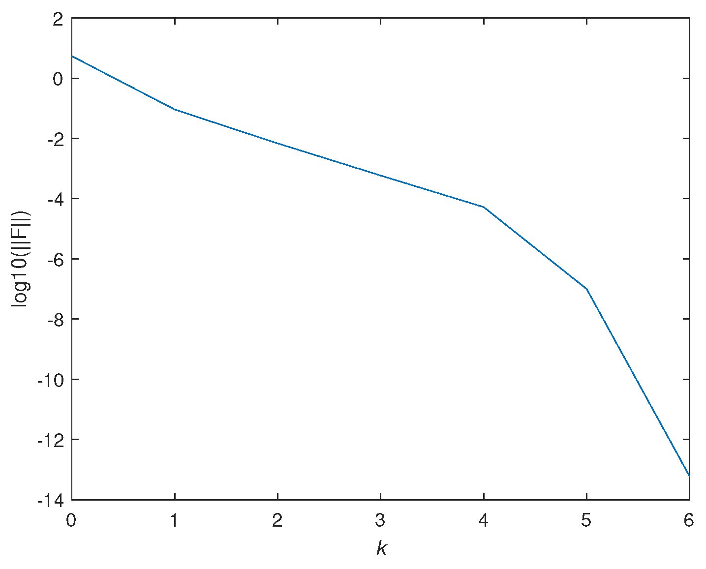
Another important aspect of our algorithm is the convergence rate of the nonlinear block. In the literature, it is reported that the JFNK method has the super-linearly convergence rate property [20,41]. We computationally verify this behavior in Figure 6. Figure 6 shows the convergence rate as a function of nonlinear iterations. To produce this figure, we use M = 2048 grid points and a fixed time step Δ t = 10 1 . The code runs until the final time t f i n a l = 1.0 with the second-order version (Crank–Nicolson-based) of the preconditioner (Section 3.4.2). Figure 6 clearly indicates that the rate of convergence of our algorithm with the new preconditioner is super linear.

4.2. Two-Dimensional Case

In Section 4.1, by solving one-dimensional test cases, we were able to demonstrate the accuracy and the effectiveness of the numerical schemes. We expect a similar performance from the algorithm when it is applied to multi-dimensional and more complicated models. This is essentially because any multi-dimensional problem can be put into a nonlinear equation form with an increasing number of components in the unknown vector. However, this is not an issue for the JFNK method, because it is known to self-consistently guarantee the convergence of all nonlinearities in the system. Indeed, just to support the above discussion, we performed a time convergence analysis by solving the two-dimensional model with the initial and boundary settings described in Section 2. Table 4 clearly verifies the second-order convergence. Figure 7 illustrates the two-dimensional performance study by employing the second-order space and time scheme. Sub-figures show the average number of Newton and GMRES iterations in time with and without using the preconditioner. With the preconditioner, the method runs extremely efficiently, needing only a few Newton and GMRES steps. This remarkable performance is due to the newly devised physics-based preconditioners and their internal multi-grid mechanism whose convergence is independent of the problem size. Here, we would like to note that we never intend to measure the CPU time performance of our algorithms. This is because such a study can depend on the computer technology and the code implementation that can vary from person to person.
Figure 8 shows the time history of the glioma cell invasion in a two-dimensional setting. Again, we start with a very high concentration of glioma cells (approximately 40 cells) in a very narrow region at the center of the computational domain ( 50 × 50 mm). The tumor concentration rapidly spreads into the high diffusion zones in approximately 50 days (third row in Figure 8). Upon hitting the low-diffusion zones, the spreading slows down for a while but the concentration starts building up and eventually reaches the steady state value (40 cells). Sub-figures in Figure 8 also indicate the sharp capturing of the tumor profiles with our second-order time and space scheme.

5. Conclusions

In this paper, we introduced a Jacobian-free Newton–Krylov method with very effective preconditioning strategies to study tumor growth dynamics. The JFNK method does not require the formation, storage, and inversion of the Jacobian matrix that make it very unique. We utilized two physics-based preconditioners which are associated with the time integration schemes to accelerate the JFNK’s convergence. Our preconditioners rely on physical models rather than prescribed matrices. This provides more practical applications and flexible coding. We solved test problems to demonstrate the numerical convergence (both in time and space) of the proposed schemes. Theoretical temporal and spatial accuracies were verified through tables. We performed efficiency studies in one- and two-dimensional settings and provided figures that illustrate the average number of linear and nonlinear iterations with and without using the preconditioners. Our study clearly indicates that the JFNK method with the new preconditioners works very well. The average number of GMRES iterations drops down to very low numbers. This is a very important conclusion because, when we apply the methodology to more complex tumor dynamics (coupled with fluid dynamics [11]), the efficiency will be crucial. We are currently working on more realistic coupled fluid dynamics and interface dynamics model with full radiotherapeutic and chemotherapeutic effects to simulate the tumor growth behavior and will report our findings in a separate journal paper.

Author Contributions

Conceptualization, S.Y.K. and E.O.; methodology, S.Y.K.; software, S.Y.K.; validation, S.Y.K. and E.O.; formal analysis, S.Y.K.; investigation, S.Y.K. and E.O.; resources, S.Y.K.; data curation, S.Y.K. and E.O.; writing—original draft preparation, S.Y.K.; writing—review and editing, S.Y.K.; visualization, S.Y.K. and E.O.; supervision, S.Y.K.; All authors have read and agreed to the published version of the manuscript.

Funding

This research received no external funding.

Data Availability Statement

Not applicable.

Conflicts of Interest

The authors declare no conflict of interest.

Appendix A

The proof of convergence of the numerical schemes is not straightforward, especially for nonlinear equations and nonlinear schemes. One practical and widely used technique is the Lax’s equivalency theorem that roughly states that a linear scheme is convergent if and only if it is consistent with the governing partial differential equations (PDE) and remains stable [45,46,47,48]. This theorem is very restrictive because it requires the governing equations being linear with smooth solutions. Thus, it is not directly useful if we are solving nonlinear PDEs. In a finite volume community, the stability concept is replaced by the Total Variation Diminishing (TVD) property for the nonlinear methods in order to achieve convergence [47,48]. This is commonly used when dealing with shock (discontinuous) problems. We note that our solutions remain smooth despite having large gradients. There is another approach called the method of frozen coefficients to analyze the convergence property of nonlinear schemes [49,50]. The main principle of this approach is that if one has an idea about the maximum value of a certain coefficient and the coefficient does not show large variation in time, then one can freeze such a coefficient while performing the convergence analysis. We adopt this approach here, because although our diffusion coefficient is discontinuous constant in time and the factors in our source term can only reach to a certain maximum value.

Appendix A.1. Stability Analysis

To apply the method of frozen coefficients, we make the following assumptions. We set the diffusion coefficient to its maximum value D = D max = 0.65 . Furthermore, notice that the source term ρ c ( 1 c c max ) has a maximum function value C 0 = ρ c max / 4 with the constant ρ . We note that, by freezing these coefficients, we practically linearize the model for which the standard stability analysis is applicable. For simplicity purposes, we consider the one-dimensional version of Equation (1). The extension of the same analysis to the two dimensional model is straightforward. Finally, we can ignore the constant source term C 0 , because, by a simple transformation c ˜ = c C 0 , the in-homogeneous equation becomes a homogeneous one. Now, we are ready to apply the procedures of the stability analysis [45,46] to the following simplified model with prescribed boundary conditions
c t = D max c x x , c x | x = 0 = 0 , c x | x = 50 = 0 .
We consider the second-order Crank–Nicolson scheme below (the analysis for the first-order scheme would be similar)
c i n + 1 c i n k = D max 2 c i + 1 n + 1 2 c i n + 1 + c i n + 1 h 2 + D max 2 c i + 1 n 2 c i n + c i n h 2
where h = Δ x and k = Δ t . Letting r = D max Δ t Δ x 2 (A2) becomes
r 2 c i 1 n + 1 + ( 1 + r ) c i n + 1 r 2 c i + 1 n + 1 = r 2 c i 1 n + ( 1 r ) c i n + r 2 c i + 1 n , i = 0 , , M 1 .
Our second-order boundary condition treatment at the left boundary leads to
c 0 n , n + 1 c 1 n , n + 1 h = 0 c 1 n , n + 1 = c 0 n , n + 1 ,
and at the right boundary we have
c M n , n + 1 c M 1 n , n + 1 h = 0 c M n , n + 1 = c M 1 n , n + 1 .
Making use of (A4) and (A5) in (A3), we have
( 1 + r 2 ) c 0 n + 1 r 2 c 1 n + 1 = ( 1 r 2 ) c 0 n + r 2 c 1 n ,
r 2 c M 2 n + 1 + ( 1 + r 2 ) c M 1 n + 1 = r 2 c M 2 n + ( 1 r 2 ) c M 1 n .
Now, considering (A3), (A6) and (A7), the numerical scheme in matrix form becomes
1 + r 2 r 2 0 0 0 r 2 ( 1 + r ) r 2 0 0 0 r 2 ( 1 + r ) r 2 0 0 0 r 2 ( 1 + r ) r 2 0 0 0 r 2 1 + r 2 Q 1 × c 0 n + 1 c 1 n + 1 c i n + 1 c M 2 n + 1 c M 1 n + 1 c n + 1 =
1 r 2 r 2 0 0 0 r 2 1 r r 2 0 0 0 r 2 1 r r 2 0 0 0 r 2 1 r r 2 0 0 0 r 2 1 r 2 Q × c 0 n c 1 n c i n c M 2 n c M 1 n c n ,
or
Q 1 c n + 1 = Q c n .
Noting that Q = 2 I Q 1 , we have Q 1 c n + 1 = ( 2 I Q 1 ) c n or c n + 1 = ( 2 Q 1 1 I ) c n or c n + 1 = Q ˜ c n with Q ˜ = ( 2 Q 1 1 I ) . Since Q 1 is a symmetric matrix, its eigenvalues are real, and if λ is an eigenvalue of Q 1 , then μ = 2 λ 1 is an eigenvalue of Q ˜ [45]. Moreover, Q 1 1 and therefore Q ˜ are also symmetric because
I = ( Q 1 Q 1 1 ) T = ( Q 1 1 ) T Q 1 T = ( Q 1 1 ) T Q 1 ( Q 1 1 ) T = Q 1 1 .
Here, we intend to utilize the Proposition 3.1.13 from the text [45] to prove the stability of the numerical scheme. For that, we use one last piece of information coming from the application of the Gerschgorin Circle theorem [45] which implies that
| λ ( 1 + r 2 ) | r 2 or | λ ( 1 + r ) | r .
By working these inequalities out, we obtain 1 λ 1 + r or 1 λ 1 + 2 r , meaning that λ 1 . Using this information, we clearly have
| μ | = | 2 λ 1 | 1 .
Putting together all the information derived above, we satisfy the hypotheses of Proposition 3.1.13, meaning that the numerical scheme is unconditionally stable.

Appendix A.2. Accuracy Analysis

The consistency or accuracy analysis usually means how accurately the numerical solution approximates the true (or analytical) solution or how accurately the analytical solution satisfies the numerical method [45]. Below, we present the consistency analysis for the Crank–Nicolson scheme, and a similar analysis can also be easily applied to the backward Euler method. The analysis is simply based on the substitution of several Taylor series into the numerical scheme. Let P and P k , h represent the analytical and numerical operators, respectively, i.e.,
P c = c t x D ( x ) c x ρ c 1 c c max ,
P k , h c = c i n + 1 c i n k 1 2 D i + 1 / 2 c i + 1 n + 1 c i n + 1 h D i 1 / 2 c i n + 1 c i 1 n + 1 h h 1 2 D i + 1 / 2 c i + 1 n c i n h D i 1 / 2 c i n c i 1 n h h 1 2 ρ c i n + 1 1 c i n + 1 c max 1 2 ρ c i n 1 c i n c max ,
where k = Δ t , h = Δ x . We say that the numerical operator is consistent with the analytical one or P k , h is consistent with P if P ϕ P k , h ϕ 0 as h , k 0 with any smooth function ϕ . Here, we also assume that the diffusion coefficient D is smooth for analysis purposes, otherwise, we had to set D to a constant maximum value as we did in Appendix A.1 and our analysis would be much easier. Moreover, since D is a function of x only, we use D = d D d x and D = d 2 D d x 2 .
We utilize the following Taylor expansions about ( i h , n k ) ,
ϕ i n + 1 = ϕ i n + k ϕ t + k 2 2 ! ϕ t t + k 3 3 ! ϕ t t t +
ϕ i + 1 n = ϕ i n + h ϕ x + h 2 2 ! ϕ x x +
ϕ i 1 n = ϕ i n h ϕ x + h 2 2 ! ϕ x x +
ϕ i + 1 n + 1 = ϕ i n + h ϕ x + k ϕ t + h 2 2 ! ϕ x x + 2 h k 2 ! ϕ x t + k 2 2 ! ϕ t t + h 3 3 ! ϕ x x x + 3 h 2 k 3 ! ϕ x x t + 3 h k 2 3 ! ϕ x t t + k 3 3 ! ϕ t t t +
ϕ i 1 n + 1 = ϕ i n h ϕ x + k ϕ t + h 2 2 ! ϕ x x + 2 h k 2 ! ϕ x t + k 2 2 ! ϕ t t h 3 3 ! ϕ x x x + 3 h 2 k 3 ! ϕ x x t + 3 h k 2 3 ! ϕ x t t + k 3 3 ! ϕ t t t +
D i + 1 / 2 = D i + 1 2 h D + h 2 4 D +
D i 1 / 2 = D i 1 2 h D + h 2 4 D +
We also need to form the following quantities,
ϕ i n + 1 ϕ i n k = ϕ t + k 2 ϕ t t + k 2 3 ! ϕ t t t +
ϕ i + 1 n + 1 ϕ i n + 1 h = ϕ x + h 2 ϕ x x + k ϕ x t + h 2 3 ! ϕ x x x + h k 2 ϕ x x t + k 2 2 ϕ x t t + h 3 4 ! ϕ x x x x + h 2 k 6 ϕ x x x t + h k 2 4 ϕ x x t t + k 3 6 ϕ x t t t +
ϕ i n + 1 ϕ i 1 n + 1 h = ϕ x h 2 ϕ x x + k ϕ x t + h 2 3 ! ϕ x x x h k 2 ϕ x x t + k 2 2 ϕ x t t h 3 4 ! ϕ x x x x + h 2 k 6 ϕ x x x t h k 2 4 ϕ x x t t + k 3 6 ϕ x t t t +
D i + 1 / 2 ϕ i + 1 n + 1 ϕ i n + 1 h D i 1 / 2 ϕ i n + 1 ϕ i 1 n + 1 h
= h D i ϕ x x + h k D i ϕ x x t + h 3 12 D i ϕ x x x x + h k 2 2 D i ϕ x x t t + h D i ϕ x + h k D i ϕ x t
+ h k 2 2 D i ϕ x t t + h 3 k 6 D i ϕ x x x t + h k 3 6 D i ϕ x t t t + h 3 4 D i ϕ x x + h 3 k 4 D i ϕ x x t
+ h 5 48 D i ϕ x x x x + h 3 k 2 8 D i ϕ x x t t + h k 2 2 D i ϕ x t t + O ( h 6 ) + O ( h k 4 ) .
D i + 1 / 2 ϕ i + 1 n ϕ i n h D i 1 / 2 ϕ i n ϕ i 1 n h = h D i ϕ x x + h k D i ϕ x + h 3 6 D i ϕ x x x + h 3 12 D i ϕ x x x x + h 3 4 D i ϕ x x + h 5 48 D i ϕ x x x x + h 5 120 D i ϕ x x x x x + O ( h 2 ) .
Using all necessary information, the new and old diffusion-related terms in (A13) become
1 2 h D i + 1 / 2 ϕ i + 1 n + 1 ϕ i n + 1 h D i 1 / 2 ϕ i n + 1 ϕ i 1 n + 1 h
1 2 h D i + 1 / 2 ϕ i + 1 n ϕ i n h D i 1 / 2 ϕ i n ϕ i 1 n h
= D i ϕ x x D i ϕ x 1 2 k D i ϕ x x t 1 2 k D i ϕ x t h 2 12 D i ϕ x x x x
h 2 4 D i ϕ x x h 2 12 D i ϕ x x x k 2 4 D i ϕ x x t t k 2 4 D i ϕ x t t h 2 k 12 D i ϕ x x x t h 2 k 8 D i ϕ x x t
1 2 k 3 D i ϕ x t t t h 2 k 2 16 D i ϕ x x t t h 4 48 D i ϕ x x x x h 4 240 D i ϕ x x x x x + O ( h 5 ) + O ( k 4 ) .
Using the necessary Taylor series, the source term in (A13) becomes
1 2 ϕ i n + 1 1 ϕ i n + 1 c max + ϕ i n 1 ϕ i n c max = ϕ i n 1 ϕ i n c max + k 2 ϕ t 1 2 ϕ i n c max + k 2 1 2 ϕ t t 1 ϕ i n c max ϕ t 2 c max + O ( k 3 ) .
Now, putting all the information from (A14) to (A27) together and dropping the indices, we have
P ϕ P k , h ϕ = k 2 ϕ t t D ϕ x x t D ϕ x t ρ ϕ t + 2 ρ ϕ ϕ t c max k 2 4 D ϕ x x t t + D ϕ x t t + k 3 D ϕ x t t t
h 2 4 D ϕ x x + k 3 D ϕ x t t t + 1 3 D ϕ x x x x + k 3 D ϕ x x x t + k 2 D i ϕ x x t t + k 2 4 D ϕ x x t t + O ( h 3 ) + O ( k 3 ) .
Notice that if we take a partial derivative of the original PDE with respect to t, then we obtain
ϕ t t D ϕ x x t D ϕ x t ρ ϕ t + 2 ρ ϕ ϕ t c max = 0 .
Now, P ϕ P k , h ϕ = O ( k 2 ) + O ( h 2 ) 0 as h , k 0 clearly assume that the coefficients and partial derivatives in (A28) are bounded. Furthermore, (A28) indicates that the order of accuracy of the numerical scheme is two in both time and space.
Finally, we will show that our boundary condition treatments are also consistent. We will do this for the left-end boundary point, but similar steps can be applied to the right boundary. We need to show that
c 1 2 n + 1 = c 0 n + 1 c 1 n + 1 h x c ( x , t ) | x = 0 0
as h 0 . As usual we replace the discrete values by the smooth function ϕ and use the following Taylor series about ( 1 2 , ( n + 1 ) k ) in (A29). Note that x = 0 corresponds to the staggered grid value of x 1 / 2 .
ϕ 0 n + 1 = ϕ 1 / 2 n + 1 + h 2 ϕ x + h 2 4.2 ! ϕ x x + h 3 8.3 ! ϕ x x x ϕ 1 n + 1 = ϕ 1 / 2 n + 1 h 2 ϕ x + h 2 4.2 ! ϕ x x h 3 8.3 ! ϕ x x x
ϕ 0 n + 1 ϕ 1 n + 1 h x ϕ ( x , t ) | x = 0 = ( h ) 2 4 ! ϕ x x x | x 1 / 2 + = O ( h 2 ) .
Clearly, as h 0 , ϕ 0 n + 1 ϕ 1 n + 1 h x ϕ ( x , t ) | x = 0 0 , as long as ϕ x x x is bounded. Equation (A31) also indicates that the second order of accuracy is preserved at this boundary.

References

  1. Martirosyan, N.L.; Rutter, E.M.; Ramey, W.L.; Kostelich, E.J.; Kuang, Y.; Preul, M.C. Mathematically modeling the biological properties of gliomas: A review. Math. Biosci. Eng. 2015, 12, 879–905. [Google Scholar] [CrossRef] [PubMed]
  2. Alfonso, J.C.L.; Talkenberger, K.; Seifert, M.; Klink, B.; Hawkins-Daarud, A.; Swanson, K.R.; Hatzikirou, H.; Deutsch, A. The biology and mathematical modelling of glioma invasion: A review. J. R. Soc. Interface 2017, 14, 20170490. [Google Scholar] [CrossRef] [PubMed]
  3. Anvari, S.; Nambiar, S.; Pang, J.; Maftoon, N. Computational Models and Simulations of Cancer Metastasis. Arch. Comput. Methods Eng. 2021, 28, 4837–4859. [Google Scholar] [CrossRef]
  4. Hormuth, D.A.; Phillips, C.; Wu, C.; Lima, E.A.B.F.; Lorenzo, G.; Jha, P.K.; Jarrett, A.M.; Oden, J.T.; Yankeelov, T.E. Biologically-Based Mathematical Modeling of Tumor Vasculature and Angiogenesis via Time-Resolved Imaging Data. Cancers 2021, 13, 3008. [Google Scholar] [CrossRef]
  5. Tunc, B.; Hormuth, D.; Biros, G.; Yankeelov, T. Modeling of Glioma Growth with Mass Effect by Longitudinal Magnetic Resonance Imaging. IEEE Trans. Biomed. Eng. 2021, 68, 3713–3724. [Google Scholar] [CrossRef] [PubMed]
  6. Wu, G.; Lee, E.; Li, G. Numerical solutions of the reaction-diffusion equation: An integral equation method using the variational iteration method. Int. J. Numer. Methods Heat Fluid Flow 2015, 25, 265–271. [Google Scholar] [CrossRef]
  7. de la Cruz, R.; Guerrero, P.; Calvo, J.; Alarcón, T. Coarse-graining and hybrid methods for efficient simulation of stochastic multi-scale models of tumour growth. J. Comput. Phys. 2017, 350, 974–991. [Google Scholar] [CrossRef] [PubMed]
  8. Adenis, L.; Plaszczynski, S.; Grammaticos, B.; Pallud, J.; Badoual, M. The Effect of Radiotherapy on Diffuse Low-Grade Gliomas Evolution: Confronting Theory with Clinical Data. J. Pers. Med. 2021, 11, 818. [Google Scholar] [CrossRef]
  9. Mach, J.; Benes, M.; Strachota, P. Nonlinear Galerkin finite element method applied to the system of reaction—Diffusion equations in one space dimension. Comput. Math. Appl. 2017, 73, 2053–2065. [Google Scholar] [CrossRef]
  10. de Montigny, J.; Iosif, A.; Breitwieser, L.; Manca, M.; Bauer, R.; Vavourakis, V. An in silico hybrid continuum-/agent-based procedure to modelling cancer development: Interrogating the interplay amongst glioma invasion, vascularity and necrosis. Methods 2021, 185, 94–104, Methods on simulation in biomedicine,. [Google Scholar] [CrossRef] [PubMed]
  11. Engwer, C.; Wenske, M. Estimating the extent of glioblastoma invasion. J. Math. Biol. 2021, 82. [Google Scholar] [CrossRef] [PubMed]
  12. Kapoor, M.; Joshi, V. Numerical approximation of 1D and 2D reaction diffusion system with modified cubic UAH tension B-spline DQM. J. Math. Comput. Sci. 2021, 11, 1650–1667. [Google Scholar]
  13. Jaroudi, R.; Baravdish, G.; Johansson, B.T.; Astrom, F. Numerical reconstruction of brain tumours. Inverse Probl. Sci. Eng. 2019, 27, 278–298. [Google Scholar] [CrossRef]
  14. Amereh, M.; Edwards, R.; Akbari, M.; Nadler, B. In-Silico Modeling of Tumor Spheroid Formation and Growth. Micromachines 2021, 12, 749. [Google Scholar] [CrossRef] [PubMed]
  15. Lipková, J.; Angelikopoulos, P.; Wu, S.; Alberts, E.; Wiestler, B.; Diehl, C.; Preibisch, C.; Pyka, T.; Combs, S.; Hadjidoukas, P.; et al. Personalized Radiotherapy Design for Glioblastoma: Integrating Mathematical Tumor Models, Multimodal Scans, and Bayesian Inference. IEEE Trans. Med. Imaging 2019, 38, 1875–1884. [Google Scholar] [CrossRef]
  16. Dehghan, M.; Narimani, N. An element-free Galerkin meshless method for simulating the behavior of cancer cell invasion of surrounding tissue. Appl. Math. Model. 2018, 59, 500–513. [Google Scholar] [CrossRef]
  17. Dehghan, M.; Narimani, N. Radial basis function-generated finite difference scheme for simulating the brain cancer growth model under radiotherapy in various types of computational domains. Comput. Methods Programs Biomed. 2020, 195, 105641. [Google Scholar] [CrossRef] [PubMed]
  18. Gaw, N.; Hawkins-Daarud, A.; Hu, L.S.; Yoon, H.; Wang, L.; Xu, Y.; Jackson, P.R.; Singleton, K.W.; Baxter, L.C.; Eschbacher, J.; et al. Integration of machine learning and mechanistic models accurately predicts variation in cell density of glioblastoma using multiparametric MRI. Sci. Rep. 2019, 9, 10063. [Google Scholar] [CrossRef] [PubMed]
  19. Ozugurlu, E. A note on the numerical approach for the reaction–diffusion problem to model the density of the tumor growth dynamics. Comput. Math. Appl. 2015, 69, 1504–1517. [Google Scholar]
  20. Knoll, D.A.; Keyes, D.E. Jacobian-Free Newton Krylov Methods: A survey of approaches and applications. J. Comput. Phys. 2004, 193, 357–397. [Google Scholar] [CrossRef]
  21. Saad, Y. Iterative Methods for Sparse Linear Systems; SIAM: Philadelphia, PA, USA, 2003. [Google Scholar]
  22. Zhang, H.; Guo, J.; Lu, J.; Li, F.; Xu, Y. The comparison between nonlinear and linear preconditioning JFNK method for transient neutronic/thermal-hydraulics coupling problem. Ann. Nucl. Energy 2019, 132, 357–368. [Google Scholar] [CrossRef]
  23. Hossain, M.A.; Alam, J.M. Assessment of a symmetry preserving JFNK method for atmospheric convection. Comput. Phys. Commun. 2021, 269, 108113. [Google Scholar] [CrossRef]
  24. Zhang, H.; Guo, J.; Lu, J.; Li, F.; Xu, Y.; Downar, T. An assessment of coupling algorithms in HTR simulator TINTE. Nucl. Sci. Eng. 2018, 190, 287–309. [Google Scholar] [CrossRef]
  25. Axelsson, O.; Blaheta, R.; Byczanski, P.; Karátson, J.; Ahmad, B. Preconditioners for regularized saddle point problems with an application for heterogeneous Darcy flow problems. J. Comput. Appl. Math. 2015, 280, 141–157. [Google Scholar] [CrossRef]
  26. Park, H.; Gaston, D.; Kadioglu, S.; Knoll, D. Tightly Coupled Multiphysics Simulations For Pebble Bed Reactors. In American Nuclear Society 2009 International Conference on Advances in Mathematics, Computational Methods and Reactor Physics; Springs: Saratoga, NY, USA, 2009; pp. 3–7. [Google Scholar]
  27. Wang, B.; Feng, Z.; Chen, Y.; Zhang, D.; Wu, Z.; Li, J.; Li, M.; Ma, R.; Li, C. Optimization and Improvement of Sodium Heated Once-through Steam Generator Transient Analysis Code Based on the JFNK Algorithm. Energies 2023, 16, 482. [Google Scholar] [CrossRef]
  28. Guo, J.; Zhang, S.; Prelim Verif, C.Y. Incompressible Navier–Stokes Equations Solved Newton Method. Int. J. Adv. Nucl. React. Desing Tech. 2020, 2, 69–85. [Google Scholar] [CrossRef]
  29. Ascher, U.M.; Greif, C. A First Course in Numerical Methods; SIAM: Philadelphia, PA, USA, 2011. [Google Scholar]
  30. Kelley, C.T. Iterative Methods for Solving Linear and Nonlinear Equations; SIAM: Philadelphia, PA, USA, 1995. [Google Scholar]
  31. Kadioglu, S.Y.; Knoll, D.A. A Jacobian-Free Newton Krylov Implicit-Explicit Time Integration Method for Incompressible Flow Problems. Commun. Comput. Phys. 2013, 13, 1408–1431. [Google Scholar] [CrossRef]
  32. Kadioglu, S.Y.; Knoll, D.A. A Fully Second Order Implicit/Explicit Time Integration Technique for Hydrodynamics Plus Nonlinear Heat Conduction Problems. J. Comput. Phys. 2010, 229, 3237–3249. [Google Scholar] [CrossRef]
  33. Kadioglu, S.Y.; Knoll, D.A.; Lowrie, R.B.; Rauenzahn, R.M. A Second Order Self-Consistent IMEX Method for Radiation Hydrodynamics. J. Comput. Phys. 2010, 229, 8313–8332. [Google Scholar] [CrossRef]
  34. Kadioglu, S. A Second-Order IMEX Method for Multi-Phase Flow Problems. Int. J. Comput. Methods 2017, 14, 1750056. [Google Scholar] [CrossRef]
  35. Kadioglu, S.Y. Analysis of the Self-Consistent IMEX Method for Tightly Coupled Non-linear Systems. J. Comp. Appl. Math. 2017, 322, 148–160. [Google Scholar] [CrossRef]
  36. Everett, R.; BFlores, K.; Henscheid, N.; Lagergren, J.; Larripa, K.; Li, D.; TNardini, J.; TTNguyen, P.; Bruce Pitman, E.; MRutter, E. A Tutorial Review of Mathematical Techniques for Quantifying Tumor Heterogeneity. Math. Biosci. Eng. 2020, 17, 3660–3709. [Google Scholar] [CrossRef] [PubMed]
  37. Murray, J. Mathematical Biology II: Spatial Models and Biomedical Applications; Springer: New York, NY, USA, 2003. [Google Scholar]
  38. Swanson, K.; Harpold, H.; Peacock, D.; Rockne, R.; Pennington, C.; Kilbride, L.; Grant, R.; Wardlaw, J.; Alvord, E.A., Jr. Velocity of radial expansion of contrast-enhancing gliomas and the effectiveness of radiotherapy in individual patients: A proof of principle. Clin. Oncol. 2008, 20, 301–308. [Google Scholar] [CrossRef] [PubMed]
  39. Shim, E.; Kwon, Y.G.; Ko, H.J. Computational Analysis of Tumor Angiogenesis Patterns Using a Two-dimensional Model. Yonsei Med. J. 2005, 46, 275–283. [Google Scholar] [CrossRef]
  40. Dembo, R.S.; Eisenstat, S.C.; Steihaug, T. Inexact Newton methods. SIAM J. Num. Anal. 1982, 19, 400–408. [Google Scholar] [CrossRef]
  41. Kelley, C.T. Solving Nonlinear Equations with Newton’s Method; SIAM: Philadelphia, PA, USA, 2003. [Google Scholar]
  42. Brown, P.; Saad, Y. Hybrid Krylov Methods for Nonlinear Systems of Equations. SIAM J. Sci. Stat. Comput. 1990, 11, 450–481. [Google Scholar] [CrossRef]
  43. Briggs, W.L. A Multigrid Tutorial; SIAM: Philadelphia, PA, USA, 2000. [Google Scholar]
  44. Zemkov, E.P.; Loskutov, A. Exact analytical solutions for nonlinear waves in the inhomogeneous Fisher-Kolmogorov equation. Eur. Phys. J. B 2011, 79, 79–84. [Google Scholar] [CrossRef]
  45. Thomas, J. Numerical Partial Differential Equations I (Finite Difference Methods); Texts in Applied Mathematics; Springer: New York, NY, USA, 1998. [Google Scholar]
  46. Strikwerda, J.C. Finite Difference Schemes Partial Differential Equations; Wadsworth & Brooks/Cole, Advance Books & Software: Pacific Grove, CA, USA, 1989. [Google Scholar]
  47. Thomas, J. Numerical Partial Differential Equations II (Conservation Laws and Elliptic Equations); Texts in Applied Mathematics; Springer: New York, NY, USA, 1999. [Google Scholar]
  48. Leveque, R.J. Finite Volume Methods for Hyperbolic Problems; Texts in Applied Mathematics; Cambridge University Press: Cambridge, UK, 1998. [Google Scholar]
  49. Mishra, S.; Svard, M. On stability of numerical schemes via frozen coefficients and the magnetic induction equation. BIT Numer. Math. 2010, 50, 85–108. [Google Scholar] [CrossRef]
  50. Appadu, A.R.; Lubuma, J.; Mphephu, N. Computational Study of three numerical methods for some linear and nonlinear advection-diffusion-reaction problems. Prog. Comput. Fluid Dyn. 2017, 17, 114–129. [Google Scholar] [CrossRef]
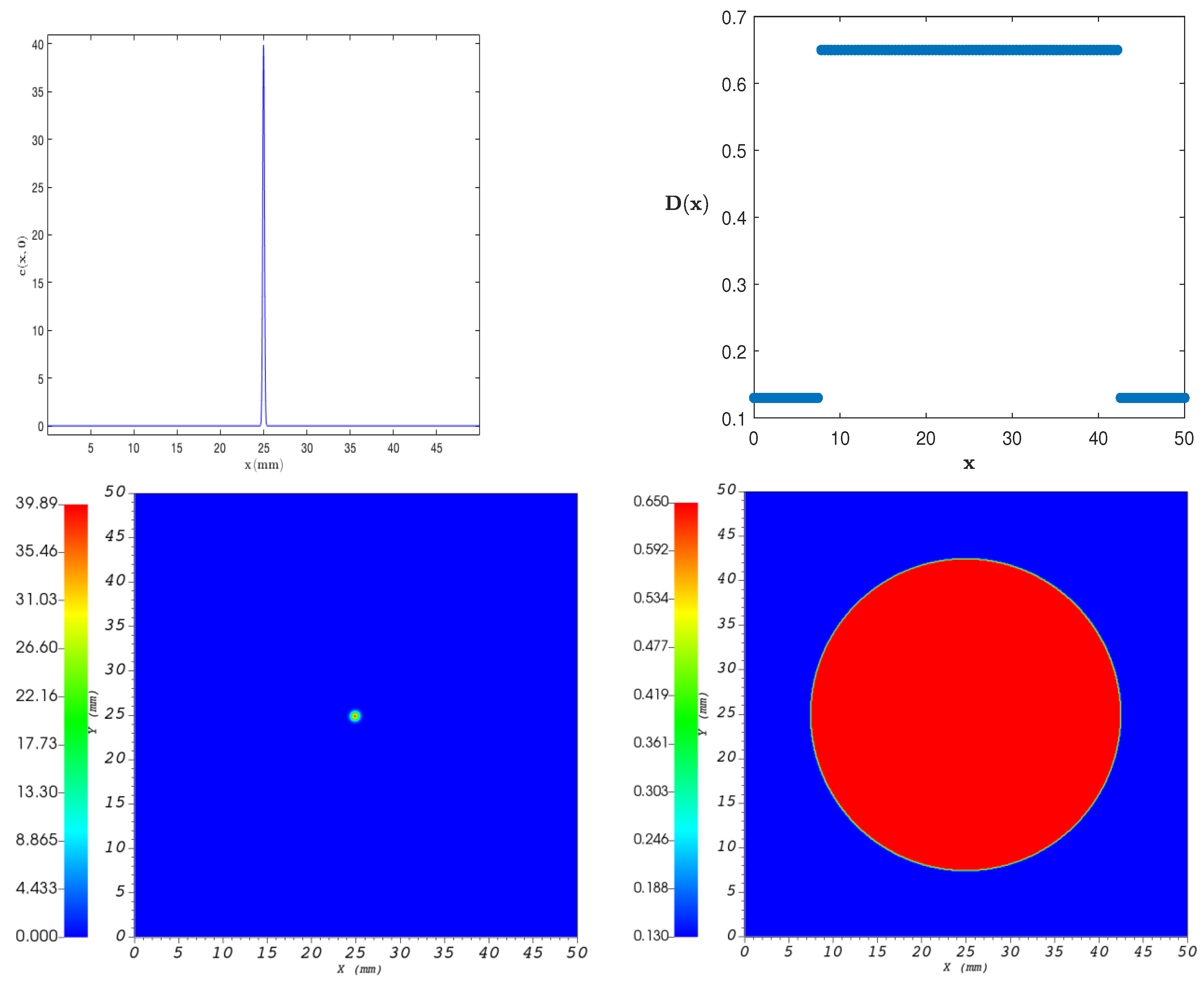
Figure 1. Left column: One- and two-dimensional initial tumor concentrations; Right column: One- and two-dimensional discontinuous diffusion coefficients.
Applsci 13 06579 g001
Figure 2. A staggered grid cell (left) and a solution representation (right).
Applsci 13 06579 g002
Figure 3. Time simulations of tumor concentration of glioma cells with ρ = 0.012   day 1 , Δ t = 0.01 14.4   min , Δ x = 50 M . Left column: M = 128 ; and right column: M = 4096 .
Applsci 13 06579 g003
Figure 4. Comparison of the results of [19] versus ours for time t = 1 , 5 , 10 , 50 .
Applsci 13 06579 g004
Figure 5. One-dimensional performance study of the preconditioners. Left column: with the CN scheme; and right column: with the BE scheme.
Applsci 13 06579 g005
Figure 6. Convergence rate as the function of nonlinear iteration for the JFNK method with the new preconditioner that utilizes the Crank–Nicolson scheme (Section 3.4.2).
Applsci 13 06579 g006
Figure 7. Two-dimensional performance study of the preconditioners with the CN time scheme.
Applsci 13 06579 g007
Figure 8. Time history of the solution profiles. First row: t = 0.1 , t = 0.2 , t = 0.5 . Second row: t = 1.0 , t = 5.0 , t = 10.0 . Third row: t = 50.0 , t = 75.0 , t = 100.0 . Fourth row: t = 250.0 , t = 500.0 , t = 1300.0 .
Applsci 13 06579 g008
Table 1. Crank–Nicolson, M = 2048 , Δ t = 10 1 .
Time Convergence Analysis with E = | | c Δ t / 2 k 1 c Δ t / 2 k | | p in Columns 1, 3, 5
p = 1 , k = 1 , , 8 Conv. Rate ( r  in (25)) p = 2 , k = 1 , , 8 Conv. Rate ( r  in (25)) p = , k = 1 , , 8 Conv. Rate ( r  in (25))
7.22 × 10 5 2.0000 4.28 × 10 5 2.0004 1.38 × 10 4 2.0005
5.55 × 10 6 2.0000 1.07 × 10 5 2.0001 3.44 × 10 5 2.0001
1.39 × 10 6 2.0029 2.67 × 10 6 1.9985 8.59 × 10 6 1.9973
3.46 × 10 7 1.9980 6.69 × 10 7 1.9992 2.15 × 10 6 1.9998
8.67 × 10 8 1.9711 1.67 × 10 7 2.0105 5.38 × 10 7 2.0172
2.21 × 10 8 1.9506 4.15 × 10 8 2.0359 1.33 × 10 7 2.0687
5.72 × 10 9 1.9014 1.01 × 10 8 2.0615 3.17 × 10 8 2.1685
1.53 × 10 9 2.42 × 10 9 7.05 × 10 9
Table 2. Backward Euler, M = 2048 , Δ t = 10 1 .
Time Convergence Analysis with E = | | c Δ t / 2 k 1 c Δ t / 2 k | | p in Columns 1, 3, 5
p = 1 , k = 1 , , 8 Conv. Rate ( r  in (25)) p = 2 , k = 1 , , 8 Conv. Rate ( r  in (25)) p = , k = 1 , , 8 Conv. Rate ( r  in (25))
1.34 × 10 3 0.9969 2.17 × 10 3 0.9984 6.56 × 10 3 0.9996
6.72 × 10 4 0.9983 1.08 × 10 3 0.9989 3.28 × 10 3 0.9989
3.36 × 10 4 0.9991 5.43 × 10 4 0.9993 1.64 × 10 3 0.9991
1.68 × 10 4 0.9995 2.71 × 10 4 0.9996 8.21 × 10 4 0.9995
8.41 × 10 5 0.9998 1.36 × 10 4 0.9998 4.11 × 10 4 0.9997
4.21 × 10 5 0.9999 6.79 × 10 5 0.9999 2.05 × 10 4 0.9998
2.10 × 10 5 0.9999 3.39 × 10 5 0.9999 1.03 × 10 4 0.9999
1.05 × 10 5 1.70 × 10 5 5.14 × 10 5
Table 3. Spatial errors and Conv. rate between sequentially refined grid solutions with Δ t = 10 5 .
Spatial Convergence Analysis with E = | | c Δ x / 2 k 1 c Δ x / 2 k | | p in Columns 1, 3, 5
p = 1 , k = 1 , , 8 Conv. Rate p = 2 , k = 1 , , 8 Conv. Rate p = , k = 1 , , 8 Conv. Rate
6.67 × 10 4 1.9975 1.93 × 10 3 1.9987 9.70 × 10 3 1.9224
1.67 × 10 4 2.0006 4.83 × 10 4 1.9985 2.56 × 10 3 1.9972
4.18 × 10 5 2.0001 1.21 × 10 4 1.9999 6.41 × 10 4 1.9994
1.04 × 10 5 2.0002 3.02 × 10 5 1.9950 1.60 × 10 4 1.9847
2.61 × 10 6 2.0015 7.57 × 10 6 2.0064 4.05 × 10 5 2.0220
6.52 × 10 7 1.9639 1.88 × 10 6 2.0005 9.97 × 10 6 2.0647
1.67 × 10 7 1.9678 4.71 × 10 7 2.0402 2.38 × 10 6 2.2178
4.27 × 10 8 1.14 × 10 7 5.12 × 10 7
Table 4. 2D: Crank–Nicolson, M x = M y = 2048 , Δ t = 10 1 .
Time Convergence Analysis with E = | | c Δ t / 2 k 1 c Δ t / 2 k | | p in Columns 1, 3, 5
p = 1 , k = 1 , , 5 Conv. Rate p = 1 , k = 1 , , 5 Conv. Rate p = , k = 1 , , 5 Conv. Rate
2.04 × 10 3 2.0007 2.66 × 10 4 2.0008 1.10 × 10 4 2.0001
5.09 × 10 4 2.0003 6.64 × 10 5 2.0002 2.76 × 10 5 2.0000
1.27 × 10 4 2.0057 1.66 × 10 5 2.0026 6.90 × 10 6 2.0030
3.17 × 10 5 2.0087 4.14 × 10 6 2.0071 1.72 × 10 6 2.0079
7.87 × 10 6 1.03 × 10 6 4.28 × 10 7
Disclaimer/Publisher’s Note: The statements, opinions and data contained in all publications are solely those of the individual author(s) and contributor(s) and not of MDPI and/or the editor(s). MDPI and/or the editor(s) disclaim responsibility for any injury to people or property resulting from any ideas, methods, instructions or products referred to in the content.