Multi-Domain Substructure Synthesis with Normalized Interpolation Technique for Non-Matching Interfaces

Abstract

The dynamic prediction of large spacecraft is a time-consuming process. The impulse-based substructuring (IBS) method is an efficient and accurate method for the dynamic analysis of large-scale structures. The ordinary IBS method couples the substructure impulse response functions (IRFs) with coincident interface nodes. However, the interface nodes in a practical structure are usually mismatched. This paper extends the ordinary IBS method and presents a method for coupling multi-domain substructures, including IBS, FEM and modal substructures, with non-matching interfaces. Both displacement compatibility and force equilibrium are satisfied on the non-matching interfaces of substructures by introducing the normalized interpolation technique into the framework of IBS. To evaluate the performance of the proposed method, numerical models and a practical application with a lunar lander and a rover are presented. The main bodies of the lander and the rover are coupled by non-matching interfaces, and the coupled system is excited by a buffer load. With the employment of this proposed method, the computing time of the landing simulation of the lunar lander is dramatically reduced, and the results show strong agreement with references. It is demonstrated that the proposed method is accurate and efficient in the transient dynamic analysis of engineering structures.

1. Introduction

As an engineering structure becomes more complex, the costs for structural dynamic analysis increase enormously. The computationally intensive design process of large-scale spacecraft needs repetitive calculations with efficient analysis techniques that provide reliable dynamic predictions. Until now, one essential tool for engineers to solve these issues has been dynamic substructuring (DS) technology.

Generally, DS methods can be categorized as the component mode synthesis (CMS) method [1,2], the frequency-based substructuring (FBS) method [3], and the impulse-based substructuring (IBS) method [4]. An overview of DS methods is provided in ref. [5]. The CMS method and the FBS method are two widely used techniques in many industrial fields, and they are relatively well-developed. However, when facing transient impact problems, such as the soft landing process of spacecraft, the CMS and FBS expose shortcomings: a large frequency band should be considered, which makes the analysis expensive and difficult to apply. The IBS method shows an advantage in dealing with transient impact problems [4,5,6].

Gordis [7] proposed the idea of assembling substructures using impulse response functions (IRFs) of substructures early in 1995. Subsequently, Rixen proposed a dual assembly of substructures, named IBS [8], in 2010. This dual form of IBS is easy to implement, and the method is achieved by using either numerical IRFs or measured IRFs [9]. The IBS method expanded the DS techniques in the time domain and was developed by following studies. Rixen and Haghighat [6] proposed a truncation and windowing procedure to limit the cost involved by the discretized convolution product inherent in the IBS method. Rixen [10] and van der Seijs used a modal projection to filter the low-frequency contributions from the IRFs, which decreased the required length of the convolution integral. Rixen [11,12] and van der Valk extended this method by allowing the assembly of structures that are composed of both substructure finite element (FE) models and substructure IRFs. Dong and Liu [13] proposed a rigid–elastic hybrid joint description method that takes the effect of both rigid and elastic connections between substructure IRFs into consideration. Zhou and Liu [14] further studied the damping and nonlinearity of joints between substructure IRFs and put the method into practice through the dynamic prediction of the landing progress of a lunar lander. Chen [15] proposed a method for the assembly of multi-domain substructures with general joints.

However, when IRFs are generated from an experiment, the support points on the interfaces of each substructure may be mismatched. Furthermore, the FE models usually have non-matching interfaces when two substructures are constructed independently by different design groups. The assembly of IRFs obtained from these FE models has to face difficulties in satisfying compatibility on non-matching interfaces. Historically, there have been three classes of methods for coupling FE models with non-matching interfaces.

One class of methods for coupling the independently established FE models with non-matching interfaces is the Lagrange multiplier method. Aminpour [16,17] presented hybrid variational formulations for the coupling through an interface and introduced the independent Lagrange multipliers as the tractions on the interface. The equations of the coupled system are obtained by using the principle of minimum potential energy. Ransom [18] formed the general-purpose finite element code using hybrid variational formulations. Park and Felippa [19] treated the interface with a displacement frame and a localized version of the method of Lagrange multipliers, and both static and dynamic partitioned structural systems were considered.

It is noteworthy that the IBS method is also based on the formulations of the classical Lagrange multipliers. However, unlike the classical approach, though the Lagrange multipliers are introduced as the interface forces, the IBS method does not introduce additional variables. After the derivation of the coupling functions, Lagrange multipliers become the only direct unknown variables, and the solution of IBS becomes concise and easy to realize (detailed in Section 2).

Another class of methods for the non-matching interfaces problem refers to the construction of transition elements. Beer [20] proposed a joint/interface element to join typical problems involving shell-to-shell and shell-to-solid interfaces. The construction of the proposed element follows the usual finite element procedure, and the stiffness matrix is obtained by the standard procedure of minimizing the total potential energy. Gens and Carol [21] developed a zero-thickness element considering the elastoplastic constitutive law. Davila [22] constructed an interface element based on the Mindlin–Reissner plate assumptions to couple solid and shell elements. However, for these approaches based on variational principles and constructing transition elements, one needs to access the shape functions of the elements over the interface, which is intrusive and complicated.

The third class of methods considers an interpolation scheme inspired by meshless methods. Kim [23] proposed an interface element method (IEM), the shape functions of which are constructed by the implementation of the moving least squares (MLS) approximations. Cho and Jun [24,25] proposed a displacement welding technique using a blended function based on the MLS function, benefiting from the meshless character of the MLS function, which can be utilized in coupled analysis of FE substructures with mismatching interfaces. Boer and van Zuijlen [26] compared different methods (nearest-neighbor interpolation, weighted residual methods and radial basis functions) that can deal with the information transfer between non-matching meshes in fluid–structure interaction computations for different criteria. Another emphasis of the interpolation scheme for non-matching interfaces is the interpolation method. The normally used interpolation methods are splines, Kriging [27] and radial basis functions [28,29]. Benefiting from consistency and the Kronecker delta function property, the Kriging interpolation function was widely used both in structural dynamics and fluid dynamics [30,31].

The assembly of FE models with non-matching interfaces can be achieved by the above-mentioned approaches. However, the framework of the IBS method is quite different from the finite element method (FEM). The IBS method is a reduced time-domain substructure method: IRFs can be regarded as “super elements in time” [12], and only limited input–output points are retained [13]. The assembly of substructure IRFs is based on the displacement compatibility of the limited discrete interface nodes, which are described directly in the physical domain [5,8]. Therefore, it is essential to study the scheme for the assembly of substructure IRFs with non-matching interfaces. To couple non-matching interface substructure IRFs for transient dynamic prediction, we use the normalized interpolation scheme and form an extended framework of the IBS method. Numerical models with efficient interpolation functions with normalization conditions (such as the moving Kriging interpolation function or the MLS function) are used to evaluate the proposed framework.

The aim of this paper is to propose a multi-domain substructure synthesis method. We consider the ordinary IBS method and present a method for coupling non-matching interfaces between substructures, including IBS, FEM and modal substructures. The work of this paper is organized as follows: First, the basic concept of the IBS method is briefly reviewed. In Section 2, the process of coupling a multi-domain substructure with non-matching interfaces is presented. In Section 4, the basic interpolation rule is detailed. In Section 5.1, numerical examples are introduced to validate the proposed method using a solid plate consisting of two parts with a plane interface. In Section 5.2, we apply this method to the dynamic prediction of a practical structure: the lunar lander with an attached rover. Finally, conclusions are drawn in Section 6.

2. Concept of Impulse-Based Substructuring Method

Rixen [4] introduced the IBS method in 2010. The basic idea of the IBS method is to describe the dynamic response of a substructure by the convolution of the IRFs’ matrix $H(t)$ and the applied force vector $f(t)$ (i.e., Duhamel’s integral) and use interface compatibility and equilibrium to assemble adjacent substructures.

The displacement vector $\mathit{u}$ of a substructure at time $t$ can be written as

$${\mathit{u}}^{(s)}\left(t\right)={\displaystyle {\int }_0^t{\mathit{H}}^{(s)}}\left(t-\tau \right){\mathit{f}}^{(s)}(\tau )d\tau$$

(1)

where superscript $s$ denotes the serial number of substructures. Applying the trapezoidal rule to Duhamel’s integral, the finite difference form of the displacement can be described approximately as

$${\mathit{u}}_n^{{}^{(s)}}={\displaystyle {\displaystyle \sum _{i=1}^{n-1}}{\mathit{H}}_{n-i}^{(s)}({\mathit{f}}_i^{(s)}+{\mathit{f}}_{i+1}^{(s)})\frac{dt}{2}}$$

(2)

where $dt$ denotes the analysis time step and n denotes the Nth analysis step. To assemble the substructures, interface displacement compatibility and interface force equilibrium are introduced. Displacement compatibility requires that the degrees of freedom on each side of the interface between any two connected substructures have to be equal. Displacement compatibility is described as

$${\displaystyle {\displaystyle \sum _{s=1}^{N_s}}{\mathit{B}}^{(s)}{\mathit{u}}^{(s)}=0}$$

(3)

where $B$ is a signed Boolean matrix identifying the matching degrees of freedom (DOF) on the interfaces, and $N_s$ is the number of substructures.

The force equilibrium requires that interface forces on each side of the interface between any two connected substructures have to be an equilibrating force system. For a matching interface assembly, the interface forces should comply with Newton’s third law. This can be described as

$${\mathit{g}}^{(s)}={\mathit{B}}^{(s)T}\mathit{\lambda }$$

(4)

where $g^{(s)}$ denotes the full set of interface forces of substructure $s$, and $\lambda$ is known as the Lagrange multiplier vector.

Combining displacement compatibility and substituting Equation (4) into Equation (2) yields the system-governing equation:

$$\left\{\begin{array}{l}{\mathit{u}}_n^{{}^{(s)}}={\displaystyle {\displaystyle \sum _{i=1}^{n-1}}{\mathit{H}}_{n-i}^{(s)}[{\mathit{f}}_i^{(s)}+{\mathit{f}}_{i+1}^{(s)}+{\mathit{B}}^{(s)T}({\mathit{\lambda }}_i+{\mathit{\lambda }}_{i+1})]\frac{dt}{2}}\\ {\displaystyle {\displaystyle \sum _{s=1}^{N_s}}{\mathit{B}}^{(s)}{\mathit{u}}^{(s)}=0}\end{array}\right.$$

(5)

Rewrite the first equation of Equation (5), and we have

$$\left\{\begin{array}{l}{\mathit{u}}_n^{{}^{(s)}}={\displaystyle {\displaystyle \sum _{i=1}^{n-2}}{\mathit{H}}_{n-i}^{(s)}[{\mathit{f}}_i^{(s)}+{\mathit{f}}_{i+1}^{(s)}+{\mathit{B}}^{(s)T}({\mathit{\lambda }}_i+{\mathit{\lambda }}_{i+1})]\frac{dt}{2}}\\ \hspace{1em}\hspace{1em}+{\mathit{H}}_1^{(s)}({\mathit{f}}_{n-1}^{(s)}+{\mathit{f}}_n^{(s)}+{\mathit{B}}^{(s)T}{\mathit{\lambda }}_{n-1})+{\mathit{H}}_1^{(s)}{\mathit{B}}^{(s)T}{\mathit{\lambda }}_n\\ {\displaystyle {\displaystyle \sum _{s=1}^{N_s}}{\mathit{B}}^{(s)}{\mathit{u}}^{(s)}=0}\end{array}\right.$$

(6)

Finally, by substituting the first line of Equation (6) into the second line of Equation (6), Lagrange multipliers ${\mathit{\lambda }}_n$ at time $t_n$ can be found as

$${\mathit{\lambda }}_n=-{\left\{{\displaystyle {\displaystyle \sum _{s=1}^{N_s}}{\mathit{B}}^{(s)}{\mathit{H}}_1^{(s)}{\mathit{B}}^{{(s)}^T}}\right\}}^{-1}{\displaystyle {\displaystyle \sum _{s=1}^{N_s}}{\mathit{B}}^{(s)}{\widehat{\mathit{u}}}_{n-1}^{(s)}}$$

(7)

where

$$\begin{array}{l}{\widehat{\mathit{u}}}_{n-1}^{(s)}={\displaystyle {\displaystyle \sum _{i=0}^{n-2}}{\mathit{H}}_{n-1}^{(s)}\left[{\mathit{f}}_i^{\left(s\right)}+{\mathit{f}}_{i+1}^{\left(s\right)}+{\mathit{B}}^{{(s)}^T}\left({\mathit{\lambda }}_i+{\mathit{\lambda }}_{i+1}\right)\right]}\\ \hspace{1em}\hspace{1em}\hspace{1em}+{\mathit{H}}_1^{(s)}\left({\mathit{f}}_{n-1}^{\left(s\right)}+{\mathit{f}}_n^{\left(s\right)}+{\mathit{B}}^{{(s)}^T}{\mathit{\lambda }}_{n-1}\right)\end{array}$$

(8)

Then, from Equation (7), we can see that Lagrange multipliers become the only direct unknown variables.

3. Assembly of Substructure with Non-Matching Interfaces

3.1. Assembly of Impulse-Based Substructures with Non-Matching Interfaces

Substructures rarely have a perfect node-to-node interface when established by different design groups. As shown in Figure 1, two substructures, ${\mathrm{\Omega }}^{(1)}$ and ${\mathrm{\Omega }}^{(2)}$, are coupled with non-matching interfaces. The nodes in each substructure’s interface are not coincident. In this case, it is necessary to reconsider the compatibility of the interface displacement and the equilibrium of the interface force. In this section, based on the work of Aminpour [16,17], who proposed an assembly method for matching interfaces, a method of assembling impulse-based substructures with non-matching interfaces is proposed.

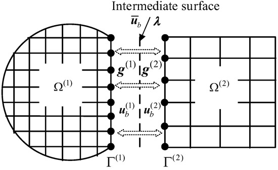
Figure 1. A two-substructure system with non-matching interfaces.

As illustrated in Figure 1, consider a structure with $N_s$ substructures. Substructure ${\mathrm{\Omega }}^{\left(s\right)}$, where superscript $s$ denotes the serial number of substructures, is coupled with other substructures with non-matching interfaces. Vector ${\mathit{u}}^{(s)}$ denotes the displacement of the substructure, ${\mathit{u}}^{(s)}$ is a constitutive of interface DOFs ${\mathit{u}}_b^{(s)}$ and internal DOFs ${\mathit{u}}_i^{(s)}$, giving

$${\mathit{u}}^{(s)}={[\begin{array}{cc}{\mathit{u}}_b^{(s)T}& {\mathit{u}}_i^{(s)T}\end{array}]}^T$$

(9)

Define a Boolean matrix ${\mathit{B}}_b^{(s)}$ that projects vector ${\mathit{u}}^{(s)}$ to vector ${\mathit{u}}_b^{(s)}$

$${\mathit{B}}_b^{(s)}{\mathit{u}}^{(s)}={\mathit{u}}_b^{(s)}$$

(10)

As the nodes in each interface of the substructure do not coincide, we consider the interface displacement compatibility and force equilibrium on an intermediate surface. Thus,

$${\overline{\mathit{u}}}_b^{(s)}={\mathit{g}}_u^{(s)}{\mathit{u}}_b^{(s)}$$

(11)

where ${\mathit{g}}_u^{(s)}$ is the interpolation function relating the interface DOFs ${\mathit{u}}_b^{(s)}$ of substructure s to the intermediate surface DOFs ${\overline{\mathit{u}}}_b^{(s)}$. Then, the displacement of substructure $s$ can be described as

$${\overline{\mathit{u}}}_b^{(s)}={\left[\begin{array}{cc}{\overline{\mathit{u}}}_b^{(s)T}& {\mathit{u}}_i^{(s)T}\end{array}\right]}^T={\left[\begin{array}{cc}{\mathit{g}}_u^{(s)}{\mathit{u}}_b^{(s)T}& {\mathit{u}}_b^{(s)T}\end{array}\right]}^T$$

(12)

The displacement compatibility is described as

$${\displaystyle {\displaystyle \sum _{s=1}^{N_s}}{\mathit{B}}^{(s)}{\overline{\mathit{u}}}^{(s)}=0}$$

(13)

$g^{(s)}$ is the interface force directly interacting with substructure $s$ and $\mathit{\lambda }$ is the Lagrange multiplier vector, which stands for the intermediate surface forces. The force equilibrium can be described as

$${\mathit{g}}^{(s)}={\mathit{g}}_f^{(s)}\left({\mathit{B}}^{(s)T}\mathit{\lambda }\right)$$

(14)

where ${\mathit{g}}_f^{(s)}$ is the force interpolation function.

Substituting Equations (13) and (14) into Equation (2) yields the system-governing equation with the non-matching interfaces

$$\left\{\begin{array}{l}{\mathit{u}}_n^{{}^{(s)}}={\displaystyle {\displaystyle \sum _{i=1}^{n-1}}{\mathit{H}}_{n-i}^{(s)}[{\mathit{f}}_i^{(s)}+{\mathit{f}}_{i+1}^{(s)}+{\mathit{B}}^{(s)T}({\mathit{\lambda }}_i+{\mathit{\lambda }}_{i+1})]\frac{dt}{2}}\\ {\displaystyle {\displaystyle \sum _{s=1}^{N_s}}{\mathit{B}}^{(s)}{\overline{\mathit{u}}}^{(s)}=0}\end{array}\right.$$

(15)

To solve this equation, the two critical interpolation functions ${\mathit{g}}_u^{(s)}$ and ${\mathit{g}}_f^{(s)}$ should be considered. Then, we assume

$${\mathit{g}}_u^{(s)}\left({\mathit{u}}_b^{(s)}\right)={\mathit{G}}_u^{(s)}{\mathit{u}}_b^{(s)}$$

(16)

$${\mathit{g}}_f^{(s)}\left({\mathit{B}}_{}^{(s)\mathrm{T}}\mathit{\lambda }\right)={\mathit{G}}_f^{(s)}{\mathit{B}}_{}^{(s)\mathrm{T}}\mathit{\lambda }$$

(17)

where ${\mathit{G}}_u^{(s)}$ and ${\mathit{G}}_f^{(s)}$ are interpolation matrices, which transform displacements and forces from substructures to intermediate surfaces, respectively.

Substituting Equation (16) into Equation (12) yields

$${\overline{\mathit{u}}}_{}^{(s)}=\left[\begin{array}{c}{\mathit{G}}_u^{(s)}{\mathit{u}}_b^{(s)}\\ {\mathit{u}}_i^{(s)}\end{array}\right]=\left[\begin{array}{cc}{\mathit{G}}_u^{(s)}& \mathbf{0}\\ \mathbf{0}& \mathit{I}\end{array}\right]\left[\begin{array}{c}{\mathit{u}}_b^{(s)}\\ {\mathit{u}}_i^{(s)}\end{array}\right]={\overline{\mathit{G}}}_u^{(s)}{\mathit{u}}_{}^{(s)}$$

(18)

where $\mathit{I}$ is the identity matrix and ${\overline{\mathit{G}}}_u^{(s)}$ is defined as

$${\overline{\mathit{G}}}_u^{(s)}=\left[\begin{array}{cc}{\mathit{G}}_u^{(s)}& \mathbf{0}\\ \mathbf{0}& \mathit{I}\end{array}\right]$$

(19)

Substituting Equations (18) and (17) into Equation (15), the non-matching interface system-governing equation is rewritten as

$$\left\{\begin{array}{l}{\mathit{u}}_n^{(s)}={\displaystyle {\displaystyle \sum _{i=0}^{n-1}}{\mathit{H}}_{n-i}^{(s)}\left[{\mathit{f}}_i^{(s)}+{\mathit{f}}_{i+1}^{(s)}+{\mathit{G}}_f^{(s)}{\mathit{B}}_{}^{(s)\mathrm{T}}{\mathit{\lambda }}_i+{\mathit{G}}_f^{(s)}{\mathit{B}}_{}^{(s)\mathrm{T}}{\mathit{\lambda }}_{i+1}^{}\right]\frac{\Delta t}{2}}\\ {\displaystyle {\displaystyle \sum _{s=1}^{N_s}}{\mathit{B}}_{}^{(s)}}{\overline{\mathit{G}}}_u^{(s)}{\mathit{u}}_n^{(s)}=\mathbf{0}\end{array}\right.$$

(20)

Similar to ordinary IBS, by solving Equation (20), ${\mathit{\lambda }}_n$ at time $t_n$ can be found as

$${\mathit{\lambda }}_n=-\left({\displaystyle {\displaystyle \sum _{s=1}^{N_s}}{\mathit{B}}^{(s)}{\overline{\mathit{G}}}_u^{(s)}{\mathit{H}}_1^{(s)}{\mathit{G}}_f^{(s)}{\mathit{B}}^{{(s)}^T}}\right){\displaystyle {\displaystyle \sum _{s=1}^{N_s}}{\mathit{B}}^{(s)}{\overline{\mathit{G}}}_u^{(s)}{\widehat{\mathit{u}}}_{n-1}^{(s)}}$$

(21)

where

$$\begin{array}{l}{\widehat{\mathit{u}}}_{n-1}^{\left(s\right)}={\displaystyle {\displaystyle \sum _{i=0}^{n-2}}{\mathit{H}}_{n-1}^{\left(s\right)}\left[{\mathit{f}}_i^{\left(s\right)}+{\mathit{f}}_{i+1}^{\left(s\right)}+{\mathit{G}}_f^{\left(s\right)}{\mathit{B}}^{{(s)}^T}\left({\mathit{\lambda }}_i+{\mathit{\lambda }}_{i+1}\right)\right]}\\ \hspace{1em}\hspace{1em}\hspace{1em}+{\mathit{H}}_1^{(s)}\left({\mathit{f}}_{n-1}^{\left(s\right)}+{\mathit{f}}_n^{\left(s\right)}+{\mathit{G}}_f^{\left(s\right)}{\mathit{B}}^{{(s)}^T}{\mathit{\lambda }}_{n-1}\right)\end{array}$$

(22)

Substituting ${\mathit{\lambda }}_n$ into Equation (20) can result in ${\mathit{u}}_n^{(s)}$. Then, ${\mathit{u}}_n^{\prime }$ and ${\mathit{u}}_n^{″}$ can be obtained through the Newmark-$\beta$ scheme

$$\left\{\begin{array}{l}{\mathit{u}}_n^{\prime }{}^{\left(s\right)}=\frac{\gamma }{\beta dt}\left({\mathit{u}}_n-{\mathit{u}}_{n-1}\right)+\left(1-\frac{\gamma }{\beta }\right){\mathit{u}}_{n-1}^{\prime }+\left(1-\frac{\gamma }{2\beta }\right)dt{\mathit{u}}_{n-1}^{″}\hfill \\ {\mathit{u}}_n^{″}{}^{\left(s\right)}=\frac{1}{\beta d{t}^2}\left({\mathit{u}}_n-{\mathit{u}}_{n-1}\right)-\frac{1}{\beta dt}{\mathit{u}}_{n-1}^{\prime }-\left(\frac{1}{2\beta }-1\right){\mathit{u}}_{n-1}^{″}\hfill \end{array}\right.$$

(23)

$\gamma =0.5$ and $\beta =0.25$ for default.

We call this substructure method non-matching interfaces IBS (NMI-IBS for short).

3.2. Assembly of IBS and Finite Element Substructures with Non-Matching Interfaces

The IBS method needs to pre-compute the impulse response of a substructure. If a substructure is often changed during the design process, generating the impulse response is much more expensive than performing the Newmark method once. So, in this section, we propose a method of assembling the IBS and finite element substructure with non-matching interfaces. The substructure that changes frequently will be modeled as an FE model and others will be represented by an IBS.

For a finite element substructure, the equations of motion can be described as

$${\mathit{M}}^{\left(r\right)}{\mathit{u}}^{″}{}^{\left(r\right)}(t)+{\mathit{C}}^{\left(r\right)}{\mathit{u}}^{\prime }{}^{\left(r\right)}(t)+\mathit{K}{\mathit{u}}^{\left(r\right)}(t)={\mathit{f}}^{\left(r\right)}\left(t\right)+{\mathit{g}}^{\left(r\right)}\left(t\right)$$

(24)

where superscript $r$ denotes the serial number of FE substructures. Separately, ${\mathit{f}}^{\left(r\right)}\left(t\right)$, ${\mathit{g}}^{\left(r\right)}\left(t\right)$ denote the external forces and interface forces acting on the FE substructure r.

Similar to Equation (12), the displacement substructure can be described as

$${\mathit{u}}^{(r)}={[\begin{array}{cc}{\overline{\mathit{u}}}_b^{(r)T}& {\mathit{u}}_i^{(r)T}\end{array}]}^T={[\begin{array}{cc}{\mathit{g}}_u^{(r)}{\left({\mathit{u}}_b^{(r)}\right)}^T& {\mathit{u}}_i^{(r)T}\end{array}]}^T$$

(25)

where ${\mathit{u}}_b^{(r)}$ and ${\mathit{u}}_i^{(r)}$ are interface DOFs and internal DOFs of finite element substructures r. ${\mathit{g}}_u^{(r)}$ is the interpolation function relating interface DOFs ${\mathit{u}}_b^{(r)}$ to the intermediate surface with coincident intermediate surface DOFs ${\overline{\mathit{u}}}_b^{(r)}$.

Then, the displacement compatibility of the IBS and FEM substructures is described as

$${\displaystyle {\displaystyle \sum _{s=1}^{N_s}}{\mathit{B}}^{(s)}{\overline{\mathit{u}}}^{(s)}+{\displaystyle {\displaystyle \sum _{s=1}^{N_r}}{\mathit{B}}^{(r)}{\overline{\mathit{u}}}^{(r)}=0}}$$

(26)

Similar to Equation (14), the interface force ${\mathit{g}}_{}^{(r)}\left(t\right)$ that directly interacts with substructure r can be described as

$${\mathit{g}}_{}^{(r)}={\mathit{g}}_f^{(r)}\left({\mathit{B}}^{(r)T}\mathit{\lambda }\right)$$

(27)

where ${\mathit{g}}_f^{(r)}$ is the force interpolation function, ${\mathit{g}}_{}^{(r)}$ is the interface forces directly interacting with the substructure and $\mathit{\lambda }$ is the Lagrange multiplier vector, which stands for the intermediate surface forces.

Substituting Equations (13), (14), (26) and (27) into Equations (2) and (24) yields the system-governing equation with non-matching interfaces

$$\left\{\begin{array}{l}{\mathit{u}}^{(s)}(t)={\displaystyle {\displaystyle \sum _{i=0}^{n-1}}{\mathit{H}}_{n-i}^{(s)}\left[{\mathit{f}}_i^{(s)}+{\mathit{f}}_{i+1}^{(s)}+{\mathit{g}}_i^{(s)}+{\mathit{g}}_{i+1}^{(s)}\right]\frac{\mathrm{d}t}{2}}\hfill \\ {\mathit{M}}_{}^{(r)}{{\mathit{u}}^{″}}^{\left(\mathit{r}\right)}\left(t\right)+{\mathit{C}}_{}^{(r)}{{\mathit{u}}^{\prime }}^{\left(\mathit{r}\right)}\left(t\right)+{\mathit{K}}_{}^{(r)}{\mathit{u}}_{}^{(r)}\left(t\right)={\mathit{f}}_{}^{(r)}\left(t\right)+{\mathit{g}}_{}^{(r)}\left(t\right)\hfill \\ {\displaystyle {\displaystyle \sum _{\mathit{s}=1}^{N_s}}{\mathit{B}}_{}^{(s)}{\overline{\mathit{u}}}_{}^{(s)}+{\displaystyle {\displaystyle \sum _{\mathit{r}=1}^{N_{\mathit{r}}}}{\mathit{B}}_{}^{(\mathit{r})}{\overline{\mathit{u}}}_{}^{(\mathit{r})}}}=\mathbf{0}\hfill \end{array}\right.$$

(28)

To solve this equation, using the same method mentioned in Section 3.1, we assume

$${\mathit{g}}_u^{(\mathit{r})}\left({\mathit{u}}_b^{(\mathit{r})}\right)={\mathit{G}}_u^{(\mathit{r})}{\mathit{u}}_b^{(\mathit{r})}$$

(29)

$${\mathit{g}}_f^{(s)}\left({\mathit{B}}_{}^{(s)\mathrm{T}}\mathit{\lambda }\right)={\mathit{G}}_f^{(s)}{\mathit{B}}_{}^{(s)\mathrm{T}}\mathit{\lambda }$$

(30)

where ${\mathit{G}}_u^{(r)}$ and ${\mathit{G}}_f^{(s)}$ are interpolation matrices, which transform displacements and forces from substructures to the intermediate surface, respectively.

Substituting Equation (29) into Equation (25) yields

$${\mathit{u}}^{(r)}={[\begin{array}{cc}{\mathit{G}}_u^{(r)}{\left({\mathit{u}}_b^{(r)}\right)}^T& {\mathit{u}}_i^{(r)T}\end{array}]}^T=\left[\begin{array}{cc}{\mathit{G}}_u^{(r)}& 0\\ 0& \mathit{I}\end{array}\right]\left[\begin{array}{c}{\mathit{u}}_b^{(r)}\\ {\mathit{u}}_i^{(r)}\end{array}\right]={\overline{\mathit{G}}}_u^{(r)}{\mathit{u}}_{}^{(r)}$$

(31)

where $\mathit{I}$ is identity matrix and ${\overline{\mathit{G}}}_u^{(r)}$ is defined as

$${\overline{\mathit{G}}}_u^{(r)}=\left[\begin{array}{cc}{\mathit{G}}_u^{(r)}& 0\\ 0& \mathit{I}\end{array}\right]$$

(32)

Substituting Equations (31) and (30) into Equation (28), the non-matching interfaces system-governing equation is rewritten as

$$\left\{\begin{array}{c}{\mathit{u}}^{\left(s\right)}\left(t\right)={\displaystyle \sum _{i=0}^{n-1}}{\mathit{H}}_{n-i}^{\left(s\right)}[{\mathit{f}}_i^{\left(s\right)}+{\mathit{f}}_{i+1}^{\left(s\right)}+{\mathit{G}}_f^{\left(s\right)}{\mathit{B}}^{\left(s\right)\mathrm{T}}{\mathit{\lambda }}_i+{\mathit{G}}_f^{\left(s\right)}{\mathit{B}}^{\left(s\right)\mathrm{T}}{\mathit{\lambda }}_{i+1}]\frac{\mathrm{d}t}{2}\hfill \\ {\mathit{M}}^{\left(r\right)}{\mathit{u}}^{″}{}^{\left(\mathit{r}\right)}\left(t\right)+{\mathit{C}}^{\left(r\right)}{\mathit{u}}^{\prime }{}^{\left(\mathit{r}\right)}\left(t\right)+{\mathit{K}}^{\left(r\right)}{\mathit{u}}^{\left(r\right)}\left(t\right)={\mathit{f}}^{\left(r\right)}\left(t\right)+{\mathit{G}}_f^{\left(\mathit{r}\right)}{\mathit{B}}^{\left(\mathit{r}\right)\mathrm{T}}{\lambda }_{\mathit{n}}\hfill \\ {\displaystyle \sum _{\mathit{s}=1}^{N_s}}{\mathit{B}}^{\left(s\right)}{\overline{\mathit{G}}}_u^{\left(s\right)}{\overline{\mathit{u}}}^{\left(s\right)}+{\displaystyle \sum _{\mathit{r}=1}^{N_{\mathit{r}}}}{\mathit{B}}^{\left(\mathit{r}\right)}{\overline{\mathit{G}}}_u^{\left(\mathit{r}\right)}{\overline{\mathit{u}}}^{\left(\mathit{r}\right)}=\mathbf{0}\hfill \end{array}\right.$$

(33)

Through the Newmark-$\beta$ scheme, the second line of Equation (33) can be rewritten as

$${\mathit{u}}_n^{(r)}={\mathit{R}}_n^{(r)}+\Delta t^2\beta {\underset{\_}{\mathit{M}}}^{{(r)}^{-1}}{\mathit{G}}_f^{(r)}{\mathit{B}}^{(r)T}\mathit{\lambda }$$

(34)

where

$$\left\{\begin{array}{l}{\underset{\_}{\mathbf{M}}}^{\left(r\right)}={\mathit{M}}^{\left(r\right)}+{\mathit{C}}^{\left(r\right)}\gamma \Delta t+{\mathit{K}}^{\left(r\right)}\Delta t^2\beta \hfill \\ {\mathit{R}}_n^{\left(r\right)}={\underset{\_}{\mathit{u}}}_n^{\left(r\right)}+\Delta t^2\beta {\underset{\_}{\mathit{M}}}^{{\left(r\right)}^{-1}}\left({\mathit{f}}_n^{\left(r\right)}-{\mathit{K}}^{\left(r\right)}{\underset{\_}{\mathit{u}}}_n^{\left(r\right)}-{\mathit{C}}^{\left(r\right)}{\underset{\_}{\mathit{u}}}_n^{{}_{{}^{\prime }}\left(r\right)}\right)\hfill \end{array}\right.$$

(35)

$$\left\{\begin{array}{l}{\underset{\_}{\mathit{u}}}_n^{{}_{{}^{\prime }}\left(r\right)}={\mathit{u}}_{n-1}^{{}_{{}^{\prime }}\left(r\right)}+\Delta t\left(1-\gamma \right){\mathit{u}}_{n-1}^{{}_{{}^{″}}\left(r\right)}\hfill \\ {\underset{\_}{\mathit{u}}}_n^{\left(r\right)}={\mathit{u}}_{n-1}^{\left(r\right)}+\Delta t\cdot {\mathit{u}}_{n-1}^{{}_{{}^{\prime }}\left(r\right)}+\Delta t^2\left(1/2-\beta \right){\mathit{u}}_{n-1}^{{}_{{}^{″}}\left(r\right)}\hfill \end{array}\right.$$

(36)

Then, Equation (33) can be rewritten as a difference scheme.

$$\left\{\begin{array}{l}{\mathit{u}}_n^{(r)}={\mathit{R}}_n^{(r)}+\Delta t^2\beta {\underset{\_}{\mathit{M}}}^{{(r)}^{-1}}{\mathit{G}}_f^{(r)}{\mathit{B}}^{(r)T}{\mathit{\lambda }}_n\\ {\mathit{u}}_n^{(s)}={\displaystyle {\displaystyle \sum _{i=0}^{n-1}}{\mathit{H}}_{n-1}^{(s)}\left[{\mathit{f}}_i^{(s)}+{\mathit{f}}_{i+1}^{(s)}+{\mathit{G}}_f^{(s)}{\mathit{B}}_{}^{(s)\mathbf{T}}{\mathit{\lambda }}_i^{}+{\mathit{G}}_f^{(s)}{\mathit{B}}_{}^{(s)\mathbf{T}}{\mathit{\lambda }}_{i+1}^{}\right]\frac{\mathrm{d}t}{2}}\\ {\displaystyle {\displaystyle \sum _{s=1}^{N_s}}{\mathit{B}}^{(s)}{\overline{\mathit{G}}}_{\mathbf{u}}^{(s)}{\overline{\mathit{u}}}_{}^{(s)}+{\displaystyle {\displaystyle \sum _{r=1}^{N_r}}{\mathit{B}}_{}^{(r)}{\overline{\mathit{G}}}_u^{(r)}{\overline{\mathit{u}}}_{}^{(r)}}}=0\end{array}\right.$$

(37)

Note that $u_n={[u_n^{(s)T},u_n^{(r)T}]}^T$, ${\mathit{G}}_u=\left[{\overline{\mathit{G}}}_u^{(s)},{\overline{\mathit{G}}}_u^{(r)}\right]$, $B_R^{}=[B_R^{(s)},B_R^{(r)}]$. By solving Equation (37), we yield

$${\mathit{B}}_R{\mathit{G}}_u{\mathit{A}}_{n-1}+{\mathit{B}}_R{\mathit{G}}_u\mathit{Q}{\mathit{\lambda }}_n=0$$

(38)

where

$${\mathit{A}}_{n-1}=\left[\begin{array}{c}{\mathit{S}}_{n-1}^{(s)}\\ {\mathit{R}}_{n-1}^{(s)}\end{array}\right],\mathit{Q}=\left[\begin{array}{c}{\mathit{H}}_1^{(s)}{\mathit{G}}_f^{(s)}{\mathit{B}}^{(s)T}\frac{\Delta t}{2}\\ \beta \Delta t^2{({\underset{\_}{\mathit{M}}}^{(r)})}^{-1}{\mathit{G}}_f^{(r)}{\mathit{B}}^{(r)T}\end{array}\right]$$

(39)

$$\begin{array}{l}{\mathit{S}}_{n-1}^{(s)}={\displaystyle {\displaystyle \sum _{i=0}^{n-2}}{\mathit{H}}_{n-2}^{(s)}\left[{\mathit{f}}_i^{(s)}+{\mathit{f}}_{i+1}^{(s)}+{\mathit{G}}_f^{(s)}{\mathit{B}}_{}^{(s)\mathbf{T}}{\mathit{\lambda }}_i^{}+{\mathit{G}}_f^{(s)}{\mathit{B}}_{}^{(s)\mathbf{T}}{\mathit{\lambda }}_{i+1}^{}\right]\frac{\mathrm{d}t}{2}}\\ \hspace{1em}\hspace{1em}\hspace{1em}+{\mathit{H}}_1^{(s)}({\mathit{f}}_{n-1}^{(s)}+{\mathit{f}}_n^{(s)}+{\mathit{G}}_f^{(s)}{\mathit{B}}_{}^{(s)\mathrm{T}}{\mathit{\lambda }}_{n-1}^{})\frac{\mathrm{d}t}{2}\end{array}$$

(40)

By solving Equation (38), ${\mathit{\lambda }}_n^{}$ as

$${\lambda }_n=-{({\mathit{B}}_R{\mathit{G}}_u\mathit{Q})}^{-1}{\mathit{B}}_R{\mathit{G}}_u{\mathit{A}}_{n-1}$$

(41)

Substituting ${\mathit{\lambda }}_n^{}$ in Equation (37) can result in ${\mathit{u}}_n^{(s)}$ and ${\mathit{u}}_n^{(r)}$.

We call this substructure method non-matching interfaces IBS-FEM (NMI-IBS-FEM for short).

3.3. Assembly of IBS and Modal Substructures with Non-Matching Interfaces

Sometimes it is much easier to obtain the modal information of structures. In this section, we will illustrate the method of assembling IBS and modal substructures with non-matching interfaces. We used the Craig–Bampton (CB) method to model the modal substructures.

The CB method is based on a consistent Rayleigh–Ritz coordinate transformation

$$\mathit{u}=\mathit{T}\eta$$

(42)

where T is a coordinate transformation matrix and $\eta$ is the generalized coordinates.

Dividing the original $\mathit{u}$ into the boundary and internal DOFs ${\mathit{u}}_b$ and ${\mathit{u}}_i$, the modal substructure formulation can be partitioned as

$$\left[\begin{array}{cc}{\mathit{M}}_{ii}^{(m)}& {\mathit{M}}_{ib}^{(m)}\\ {\mathit{M}}_{bi}^{(m)}& {\mathit{M}}_{bb}^{(m)}\end{array}\right]\left[\begin{array}{c}{\mathit{u}}_i^{″}{}^{(m)}\\ {\mathit{u}}_b^{″}{}^{(m)}\end{array}\right]+\left[\begin{array}{cc}{\mathit{C}}_{ii}^{(m)}& {\mathit{C}}_{ib}^{(m)}\\ {\mathit{C}}_{bi}^{(m)}& {\mathit{C}}_{bb}^{(m)}\end{array}\right]\left[\begin{array}{c}{\mathit{u}}_i^{\prime }{}^{(m)}\\ {\mathit{u}}_b^{\prime }{}^{(m)}\end{array}\right]+\left[\begin{array}{cc}{\mathit{K}}_{ii}^{(m)}& {\mathit{K}}_{ib}^{(m)}\\ {\mathit{K}}_{bi}^{(m)}& {\mathit{K}}_{bb}^{(m)}\end{array}\right]\left[\begin{array}{c}{\mathit{u}}_i^{(m)}\\ {\mathit{u}}_b^{(m)}\end{array}\right]=\left[\begin{array}{c}{\mathit{f}}_i^{(m)}\\ {\mathit{g}}_b^{(m)}\end{array}\right]$$

(43)

where the superscript m denotes the serial number of modal substructures.

According to the CB method [1], the constraint modes are defined as

$${\mathrm{\Phi }}_c^{(m)}=\left[\begin{array}{c}-{(K_{ii}^{(m)})}^{-1}{K}_{ib}^{(m)}\\ \mathit{I}\end{array}\right]$$

(44)

To obtain the fixed-interface modes, the substructure is assumed to be fixed at its boundary DOF ${\mathit{u}}_b^m$ and, from Equation (43), the eigen equation of the fixed substructure is

$${\mathit{M}}_{ii}^{\left(m\right)}{\mathit{u}}_i^{″}{}^{\left(m\right)}+{\mathit{K}}_{ii}^{\left(m\right)}{\mathit{u}}_i^{\left(m\right)}=0$$

(45)

The fixed-interface modes ${\mathrm{\Phi }}_b^{(m)}$ are mass normalized and are

$${\mathrm{\Phi }}_B^{{(m)}^{\mathrm{T}}}{\mathit{M}}_{ii}^{(m)}{\mathrm{\Phi }}_B^{(m)}=\mathit{I},{\mathrm{\Phi }}_B^{{(m)}^{\mathrm{T}}}{\mathit{K}}_{ii}^{(m)}{\mathrm{\Phi }}_B^{(m)}={\mathit{\Lambda }}^{(m)}$$

(46)

where ${\mathit{\Lambda }}^{(m)}$ is a diagonal matrix whose elements are the squares of the corresponding eigenfrequencies of the fixed substructure.

In the CB method,

$${\mathit{u}}_i^{(m)}={\mathrm{\Phi }}_B^{(m)}{\mathit{\eta }}_B^{(m)}+{\mathrm{\Phi }}_{Ci}^{(m)}{\mathit{u}}_b^{(m)}$$

(47)

where ${\mathit{\eta }}_B^{(m)}$ is the fixed-interface generalized coordinates, and ${\mathrm{\Phi }}_{Ci}^{(m)}=-{(K_{ii}^{(m)})}^{-1}{K}_{ib}^{(m)}$ is the partition of constraint modes associated with the internal DOFs.

Then, the coordinate transformation can be described as

$$u^{(m)}=\left[\begin{array}{cc}{\mathrm{\Phi }}_B^{(m)}& {\mathrm{\Phi }}_{Ci}^{(m)}\\ 0& \mathit{I}\end{array}\right]\left[\begin{array}{c}{\mathit{\eta }}_B^{(m)}\\ {\mathit{u}}_b^{(m)}\end{array}\right]={\mathit{T}}^{(m)}{\mathit{\eta }}^{(m)}$$

(48)

where ${\mathit{T}}^{(m)}$ is the reduction matrix of the Craig–Bampton method.

In Equation (48), all boundary DOFs are retained. Usually, not all eigenvectors are retained for ${\mathrm{\Phi }}_B^{(m)}$ and that will result in a reduction of the substructure.

According to Equation (48), the modal substructures are given as

$${\overline{\mathit{M}}}_{}^{(m)}{{\mathit{\eta }}^{″}}_{}^{(m)}\left(t\right)+{\overline{\mathit{C}}}_{}^{(m)}{{\mathit{\eta }}^{\prime }}_{}^{(m)}\left(t\right)+{\overline{\mathit{K}}}_{}^{(m)}{\mathit{\eta }}_{}^{(m)}\left(t\right)={\overline{\mathit{f}}}_{}^{(m)}\left(t\right)+{\mathit{T}}_{}^{(m)}{}_{}^{\mathrm{T}}{\mathit{g}}_{}^{(m)}\left(t\right)$$

(49)

where ${\overline{\mathit{M}}}_{}^{(m)}={\mathit{T}}_{}^{(m)\mathrm{T}}{\mathit{M}}_{}^{(m)}{\mathit{T}}_{}^{(m)}$, ${\overline{\mathit{C}}}_{}^{(m)}={\mathit{T}}_{}^{(m)\mathrm{T}}{\mathit{C}}_{}^{(m)}{\mathit{T}}_{}^{(m)}$, ${\overline{\mathit{K}}}_{}^{(m)}={\mathit{T}}_{}^{(m)\mathrm{T}}{\mathit{K}}_{}^{(m)}{\mathit{T}}_{}^{(m)}$, and ${\overline{\mathit{f}}}_{}^{(m)}={\mathit{T}}_{}^{(m)}{\mathit{f}}_{}^{(m)}$.

Then, the formulation of the assembled system considering non-matching interfaces can be described as

$$\left\{\begin{array}{c}{\mathit{u}}^{\left(s\right)}\left(t\right)={\displaystyle \sum _{i=0}^{n-1}}{\mathit{H}}_{n-i}^{\left(s\right)}\left[{\mathit{f}}_i^{\left(s\right)}+{\mathit{f}}_{i+1}^{\left(s\right)}+{\mathit{G}}_f^{\left(s\right)}{\mathit{B}}^{\left(s\right)\mathrm{T}}{\mathit{\lambda }}_i+{\mathit{G}}_f^{\left(s\right)}{\mathit{B}}^{\left(s\right)\mathrm{T}}{\mathit{\lambda }}_{i+1}\right]\frac{\mathrm{d}t}{2}\hfill \\ {\overline{\mathit{M}}}^{\left(m\right)}{\mathit{\eta }}^{″}{}^{\left(\mathit{m}\right)}\left(t\right)+{\overline{\mathit{C}}}^{\left(m\right)}{\mathit{\eta }}^{\prime }{}^{\left(\mathit{m}\right)}\left(t\right)+{\overline{\mathit{K}}}^{\left(m\right)}{\mathit{\eta }}^{\left(m\right)}\left(t\right)={\overline{\mathit{f}}}^{\left(m\right)}\left(t\right)+{\mathit{T}}^{\left(m\right)\mathrm{T}}{\mathit{G}}_f^{\left(\mathit{r}\right)}{\mathit{B}}^{\left(m\right)\mathrm{T}}\mathit{\lambda }\left(t\right)\hfill \\ {\displaystyle \sum _{\mathit{s}=1}^{N_s}}{\mathit{B}}^{\left(s\right)}{\overline{\mathit{G}}}_u^{\left(s\right)}{\overline{\mathit{u}}}^{\left(s\right)}+{\displaystyle \sum _{\mathit{m}=1}^{N_{\mathit{m}}}}{\mathit{B}}^{\left(\mathit{m}\right)}{\overline{\mathit{G}}}_u^{\left(\mathit{m}\right)}{\overline{\mathit{u}}}^{\left(\mathit{m}\right)}=\mathbf{0}\hfill \end{array}\right.$$

(50)

It is easy to see that Equations (33) and (50) have the same form, so they can be solved in the same way.

We call this substructure method non-matching interfaces IBS-CB (NMI-IBS-CB for short).

4. Basic Interpolation Rule and Interpolation Functions

4.1. Basic Interpolation Rule and Interpolation Functions

As stated above, Equation (15) already satisfies displacement compatibility. However, the equivalent system of forces on the intermediate surface is not guaranteed, and an additional condition has to be introduced that is based on the conservation of energy through the interface [26,32].

The kinematic boundary condition on a continuous interface, $\mathrm{\Gamma }$, leads to

$$\delta {\mathit{u}}_{}^{(1)}=\delta {\mathit{u}}_{}^{(2)}$$

(51)

where $\delta {\mathit{u}}_{}^{(\mathit{s})}$ is the virtual displacement on the interface of substructure $s$. For two substructures with non-matching interfaces ${\mathrm{\Gamma }}^{(s)}$, there is ${\mathrm{\Gamma }}_{}^{(1)}\ne {\mathrm{\Gamma }}_{}^{(2)}$, and the virtual displacement vectors $\delta {\mathit{u}}_{}^{(\mathit{s})}$ on each discrete interface have the relationship

$$\delta {\mathit{u}}_f={\mathit{G}}_u^{(1)}\delta {\mathit{u}}_{}^{(1)}={\mathit{G}}_u^{(2)}\delta {\mathit{u}}_{}^{(2)}$$

(52)

where $\delta {\mathit{u}}_f$ is the discrete virtual displacement vectors of the intermediate surface. Thus,

$$\delta {\mathit{u}}_{}^{(1)}={\left({\mathit{G}}_u^{(1)}\right)}_{}^{-1}{\mathit{G}}_u^{(2)}\delta {\mathit{u}}_{}^{(2)}$$

(53)

The virtual work of each side of the interface force ${\mathit{g}}^{(s)}$ acting on interface ${\mathrm{\Gamma }}^{(s)}$ can be described separately as

$$\delta w_{}^{(1)}={\mathit{g}}_{}^{\left(1\right)\mathrm{T}}\delta {\mathit{u}}_{}^{\left(1\right)}$$

(54)

$$\delta w_{}^{(2)}={\mathit{g}}_{}^{\left(2\right)\mathrm{T}}\delta {\mathit{u}}_{}^{\left(2\right)}$$

(55)

Considering Equation (14), Equation (17) and ${\mathit{B}}^{(1)T}{\mathit{\lambda }}^{(1)}=-{\mathit{B}}^{(2)T}{\mathit{\lambda }}^{(2)}$, there is

$${\mathit{g}}_{}^{(1)}=-{\mathit{G}}_f^{(1)}{\left({\mathit{G}}_f^{(2)}\right)}^{-1}{\mathit{g}}_{}^{(2)}$$

(56)

Substituting (53) and (56) into (54) yields

$$\begin{array}{l}\delta w_{}^{(1)}={\left(-{\mathit{G}}_f^{(1)}{\left({\mathit{G}}_f^{(2)}\right)}^{-1}{\mathit{g}}_{}^{(2)}\right)}_{}^{\mathrm{T}}{\left({\mathit{G}}_u^{(1)}\right)}_{}^{-1}{\mathit{G}}_u^{(2)}\delta {\mathit{u}}_{}^{(2)}\\ \hspace{1em}\hspace{1em}\hspace{1em}=-{\mathit{g}}_{}^{(2)\mathrm{T}}\left({\left({\mathit{G}}_f^{(2)}\right)}^{-\mathrm{T}}{\mathit{G}}_f^{(1)\mathrm{T}}{\left({\mathit{G}}_u^{(1)}\right)}_{}^{-1}{\mathit{G}}_u^{(2)}\right)\delta {\mathit{u}}_{}^{(2)}\end{array}$$

(57)

Since there are no external forces, the energy is preserved, and there is

$$\delta w_{}^{(1)}+\delta w_{}^{(2)}=0$$

(58)

Substituting (55) and (57) into (58) yields

$${\mathit{g}}_{}^{(2)\mathrm{T}}\left({\left({\mathit{G}}_f^{(2)}\right)}^{-\mathrm{T}}{\mathit{G}}_f^{(1)}{}_{}^{\mathrm{T}}{\left({\mathit{G}}_u^{(1)}\right)}_{}^{-1}{\mathit{G}}_u^{(2)}\right)\delta {\mathit{u}}_{}^{(2)}={\mathit{g}}_{}^{(2)}{}_{}^{\mathrm{T}}\delta {\mathit{u}}_{}^{(2)}$$

(59)

Without loss of generality, we assume

$${\left({\mathit{G}}_f^{(2)}\right)}^{-\mathrm{T}}{\mathit{G}}_f^{(1)\mathrm{T}}{\left({\mathit{G}}_u^{(1)}\right)}_{}^{-1}{\mathit{G}}_u^{(2)}=\mathit{I}$$

(60)

where $\mathit{I}$ is the identity matrix, then Equation (59) is satisfied, and thus the energy through the interface is conserved. According to Farhat’s work [26], if we set the intermediate surface nodes to coincide with one of the substructure’s interfaces, such as ${\mathrm{\Gamma }}^{(1)}$ shown in Figure 1, then ${\mathit{G}}_u^{(1)}=\mathit{I}, {\mathit{G}}_f^{(1)}=\mathit{I}$ and

$${\left({\mathit{G}}_u^{(2)}\right)}_{}^{\mathrm{T}}={\mathit{G}}_f^{(2)}$$

(61)

Then, the displacement and forces on the interfaces between the two substructures have a brief relationship:

$$\left\{\begin{array}{l}{\mathit{u}}_b^{(1)}={\mathit{G}}_u^{(2)}{\mathit{u}}_b^{(2)}\\ -{\left({\mathit{G}}_u^{(2)}\right)}_{}^{\mathrm{T}}{\mathit{g}}_{}^{(1)}={\mathit{g}}_{}^{(2)}\end{array}\right.$$

(62)

Reconsidering the force equilibrium between two substructures and using the relation expressed by Equation (60), it is not difficult to obtain

$${\displaystyle {\displaystyle \sum _{i=1}^{N1}}{\mathit{g}}_{[i]}^{(1)}}=-{\displaystyle {\displaystyle \sum _{j=1}^{N2}}{\mathit{g}}_{[j]}^{(2)}}={\displaystyle {\displaystyle \sum _{j=1}^{N2}}{\displaystyle {\displaystyle \sum _{i=1}^{N1}}{\left({\mathit{G}}_{u[i,j]}^{(2)}\right)}_{}^{\mathrm{T}}{\mathit{g}}_{[i]}^{(1)}}}={\displaystyle {\displaystyle \sum _{j=1}^{N2}}{\left({\mathit{G}}_{u[i,j]}^{(2)}\right)}_{}^{\mathrm{T}}{\displaystyle {\displaystyle \sum _{i=1}^{N1}}{\mathit{g}}_{[i]}^{(1)}}}$$

(63)

where ${\left[•\right]}_{[i,j]}^{}$ is the matrix element in the row $i$ and column $j$, ${\left[•\right]}_{[i]}^{}$ is the vector element in the row $i$, and N1 and N2 are the row numbers of ${\mathit{g}}_{}^{(1)}$ and ${\mathit{g}}_{}^{(2)}$, respectively.

From Equation (63), it is easy to obtain

$${\displaystyle {\displaystyle \sum _{j=1}^{N2}}{\left({\mathit{G}}_{u[i,j]}^{(2)}\right)}_{}^{\mathrm{T}}}={\displaystyle {\displaystyle \sum _{j=1}^{N2}}{\mathit{G}}_{f[j,i]}^{(2)}}=1$$

(64)

Equation (64) shows that the sum of the rows of the displacement interpolation matrix ${\mathit{G}}_u^{(2)}$ equal to 1, which means that the force on the interface satisfies global conservation.

In short, the basic rule for the assembly of two substructures should follow Equation (53) (the inverse matrix exists), Equation (62) (the force equilibrium) and Equation (61) (the energy conservation). For more than two substructures, the interpolation matrices can be obtained successively on an intermediate surface between each of the two connected substructures.

Considering the basic rule for forming the interpolation matrix, in this paper we chose two representative interpolation methods used for non-matching interface problems: the moving Kriging interpolation and the moving least squares interpolation. Using proper parameters, both the moving Kriging and the moving least squares interpolation functions satisfy the normalization condition [23,31].

4.2. Moving Kriging and Moving Least Squares Interpolation Methods

In this section, two interpolation methods are introduced to build an interpolation matrix: the moving Kriging and moving least squares interpolation functions. Both methods satisfy the normalization condition.

The moving Kriging (MK) interpolation method is based on the work of D. G. Krige [27]. The moving Kriging interpolation $u\left(x\right)$ is defined by

$$\mathit{u}\left(x\right)=p^T\left(x\right)\mathit{S}\mathit{U}+r{\left(x\right)}^T{\mathit{R}}^{-1}\left(I-\mathit{P}\mathit{S}\right)\mathit{U}$$

(65)

$$\mathit{U}=\left[\begin{array}{c}\mathit{u}\left(x_1\right)\\ ⋮\\ \mathit{u}\left(x_n\right)\end{array}\right]$$

(66)

where $\mathit{P}$, $\mathit{R}$, $r\left(x\right)$ and $\mathit{S}$ are given by Equations (67)–(70), respectively.

$$\mathit{P}=\left[\begin{array}{ccccc}\mathit{p}({\mathit{x}}_1^{})\hspace{1em}& \cdots & \hspace{1em}\mathit{p}({\mathit{x}}_i^{})\hspace{1em}& \cdots & \hspace{1em}\mathit{p}({\mathit{x}}_n^{})\end{array}\right]$$

(67)

$$\mathit{R}=\left[\begin{array}{cccc}1& R\left({\mathit{x}}_1^{},{\mathit{x}}_2^{}\right)& \cdots & R\left({\mathit{x}}_1^{},{\mathit{x}}_n^{}\right)\\ R\left({\mathit{x}}_2^{},{\mathit{x}}_1^{}\right)& 1& \cdots & R\left({\mathit{x}}_2^{},{\mathit{x}}_n^{}\right)\\ ⋮& ⋮& \ddots & ⋮\\ R\left({\mathit{x}}_n^{},{\mathit{x}}_1^{}\right)& R\left({\mathit{x}}_n^{},{\mathit{x}}_2^{}\right)& \cdots & 1\end{array}\right]$$

(68)

$$\mathit{r}\left(\mathit{x}\right)=\left[\begin{array}{ccccc}\mathit{R}({\mathit{x}}_1^{},\mathit{x})\hspace{1em}& \cdots & \mathit{R}({\mathit{x}}_i^{},\mathit{x})\hspace{1em}& \cdots & \hspace{1em}\mathit{R}({\mathit{x}}_n^{},\mathit{x})\end{array}\right]$$

(69)

$$\mathit{S}={\left({\mathit{P}}_{}^{\mathrm{T}}{\mathit{R}}_{}^{-1}\mathit{P}\right)}_{}^{-1}{\mathit{P}}_{}^{\mathrm{T}}{\mathit{R}}_{}^{-1}$$

(70)

$R\left(x_i,x_j\right)$ is the correlation function between any two of the n nodes, $x_i$ and $x_j$. $p\left(x\right)$ is a polynomial basis given by Equation (71), and m denotes the number of terms in the basis.

$$\mathit{p}{(\mathit{x})}_{}^{\mathrm{T}}=\left[\begin{array}{cccccc}1& x& y& x^2& y^2& xy\end{array}\right]$$

(71)

We can introduce the notation

$$\mathit{B}={\mathit{R}}^{-1}\left(\mathit{I}-\mathit{P}\mathit{S}\right)$$

(72)

Then, Equation (65) can be rewritten as:

$$\mathit{u}\left(x\right)=\left[p^T\left(x\right)\mathit{S}+r{\left(x\right)}^T\mathit{B}\right]\mathit{U}={\displaystyle {\displaystyle \sum _{i=1}^{n_c}}{\varphi }_i\left(x\right)}{u}_i=\phi \left(x\right)\mathit{U}$$

(73)

where

$${\varphi }_i\left(x\right)={\displaystyle {\displaystyle \sum _{j=1}^m}{p}_j\left(x\right){\mathit{S}}_{ji}}+{\displaystyle {\displaystyle \sum _{k=1}^{n_c}}{r}_k{\left(x\right)}^T{\mathit{B}}_{ki}}$$

(74)

According to [26], the shape function ${\varphi }_i\left(x\right)$ has the characteristic that ${\displaystyle {\displaystyle \sum _i^n}{\varphi }_i^{}}=1$, which satisfies Equation (64). So, the MK interpolation method satisfies the normalization condition and could be used for the assembly of two substructures.

Similar to the MK approximation, the moving least squares interpolation $u\left(x\right)$ can be defined by

$$\mathit{u}\left(x\right)=p_{}^{\mathbf{T}}(x)\mathit{A}{(\mathit{x})}_{}^{-1}\mathit{B}(\mathit{x})\mathit{U}=\mathrm{\Phi }(\mathit{x})\mathit{U}$$

(75)

where $\mathit{A}(\mathit{x})$ and $\mathit{B}(\mathit{x})$ can be defined by

$$\mathit{A}(\mathit{x})={\displaystyle {\displaystyle \sum _{i=1}^n}\mathit{R}(\mathit{x},{\mathit{x}}_i^{})\mathit{p}({\mathit{x}}_i){\mathit{p}}_{}^{\mathbf{T}}({\mathit{x}}_i)}$$

(76)

$$\mathit{B}(\mathit{x})=\left[\begin{array}{ccc}R(\mathit{x},{\mathit{x}}_1^{})\mathit{p}({\mathit{x}}_1)& \cdots & R(\mathit{x},{\mathit{x}}_n^{})\mathit{p}({\mathit{x}}_n^{})\end{array}\right]$$

(77)

According to [26], the MLS interpolation method also satisfies the normalization condition and could be used for the assembly of two substructures.

5. Numerical Examples

5.1. Solid Plate Numerical Example

A numerical example is proposed to validate the method: the dynamic performance of a solid plate.

The solid plate is composed of two independent parts of the same size: $1000 \mathrm{mm}\times 500 \mathrm{mm}\times 30 \mathrm{mm}$. One side of the solid plate is fixed, and on the opposite side, there is a loading point and a response point, as shown in Figure 2. The two parts are directly connected on the interface.

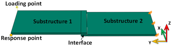
Figure 2. A solid plate assembled with plane interface.

The external force acting on the loading point lasts for 0.1 s:

$$\mathit{f}=\left\{\begin{array}{cc}40t& 0\le t\le 0.025\\ 1& 0.025\le t\le 0.050\\ 3-40t& 0.050\le t\le 0.075\\ 0& 0.075\le t\le 0.1\end{array}N\right.$$

(78)

The FE model is shown in Figure 3. The two FE substructures with coincident interface nodes are tied by a multi-point constraint (MPC).

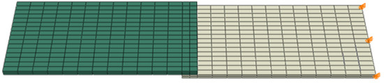
Figure 3. Two FE substructures with coincident interface nodes.

First, to implement the interpolation function, the assembly of the IBS method is discussed. To implement the IBS method, the IRFs matrix is obtained using FEM (shown in Figure 4). The IRF matrix of Substructure 1 is obtained under the free boundary condition, and Substructure 2 is one-side fixed.

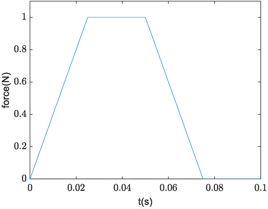
Figure 4. External force against time.

To validate the method, the support nodes on the interface are purposely chosen differently from each grid. In Substructure 1, only 18 points are extracted on the interface, and there are 34 interface points in Substructure 2. Each point has three translational DOFs. The interface has a size of $500 \mathrm{mm}\times 80 \mathrm{mm}$ and the distribution of the interface support nodes of the substructures is shown in Figure 5, yellow circles represent for interface node.

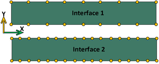
Figure 5. Interface node distribution of two solid substructures.

In this configuration, we set the intermediate surface nodes to coincide with Interface 2.

Then, ${\mathit{G}}_u^{(2)}=\mathit{I}$, ${\mathit{G}}_f^{(2)}=\mathit{I}$ and

$$\left\{\begin{array}{l}{\mathit{u}}_b^{(2)}={\mathit{G}}_u^{(1)}{\mathit{u}}_b^{(1)}\\ {\mathit{g}}^{(2)}={\mathit{B}}^{(2)\mathrm{T}}\mathit{\lambda }\\ {\mathit{g}}^{(1)}=-{\mathit{G}}_f^{(1)}{\mathit{B}}^{(1)\mathrm{T}}\mathit{\lambda }\end{array}\right.$$

(79)

where ${\mathit{G}}_f^{(1)}={\mathit{G}}_u^{(1)\mathrm{T}}$, considering the conservation of energy, and ${\mathit{B}}^{(1)}={\mathit{B}}^{(2)}=\mathit{I}$ since there is only one intermediate surface in this configuration.

In order to obtain ${\mathit{G}}_u^{(1)}$, the moving Kriging shape function matrix is employed [31]:

$$\mathit{R}\left({\mathit{x}}_i,{\mathit{x}}_j\right)=\left\{\begin{array}{l}\exp (-{(\alpha h/h_c)}^2)\hspace{1em}\hspace{1em}\hspace{1em}\hspace{1em}h\le h_c\\ 0\hspace{1em}\hspace{1em}\hspace{1em}\hspace{1em}\hspace{1em}\hspace{1em}\hspace{1em}\hspace{1em}\hspace{1em}\hspace{1em}h>h_c\end{array}\right.$$

(80)

where $h$ denotes the Euclidean distance between the given interpolation nodes ${\mathit{x}}_i$ and ${\mathit{x}}_j$, $h_c$ is the radius of the compact support domain, and $\alpha$ is the correlation coefficient to fit the model, which should be chosen properly. Using different correlation coefficients $\alpha$ will obtain results with different precision levels. While using the moving least squares interpolation to obtain ${\mathit{G}}_u^{(1)}$, we employ a weight function model with the same expression as in Equation (71) [33].

First, we set the radius of the compact support domain $h_c=85$ and $\alpha =1$. On the interface, displacement compatibility is naturally satisfied in Equation (15). For both the moving Kriging and moving least squares interpolation schemes, the sum of interface forces of direction Y on the two sides is in the order of ${10}^{-14}$ (equal to zero, the force equilibrium satisfied), as shown in Figure 6.

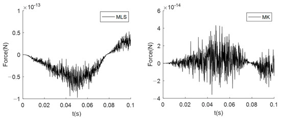
Figure 6. The sum of interface forces of direction Y.

The displacement, velocity and acceleration of the response point are used to illustrate the performance of the method. The analysis results in the Z direction are compared in Figure 7.

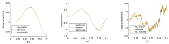
Figure 7. Comparison between the NMI-IBS and the reference for the solid plate.

We used R-squared (R2) and the relative average absolute error (RAAE) [27] to illustrate accuracy. The R2 and RAAE are computed using:

$$R^2=1-{\displaystyle {\displaystyle \sum _{i=1}^n}{({\mathit{y}}_i-{\widehat{\mathit{y}}}_i)}^2}/{\displaystyle {\displaystyle \sum _{i=1}^n}{({\mathit{y}}_i-{\overline{\mathit{y}}}_i)}^2}$$

(81)

$$\mathrm{RAAE}=\frac{{\displaystyle {\displaystyle \sum _{i=1}^n}|{\mathit{y}}_i-{\widehat{\mathit{y}}}_i|}}{n\times \mathrm{STD}}$$

(82)

where $n$ is the length of response data; ${\mathit{y}}_i$ and ${\widehat{\mathit{y}}}_i$ are the acceleration response results of the FEM and IBS methods, respectively; ${\overline{\mathit{y}}}_i$ and STD are, respectively, the mean and standard deviation of the FEM result. The accuracy of NMI-IBS is presented in Table 1.

Table 1. Accuracy of the NMI-IBS for response of the solid plate in Z direction.

	R2		RAAE
	NMI-IBS-MK	NMI-IBS-MSL	NMI-IBS-MK	NMI-IBS-MSL
Displacement	0.99987	0.99986	0.00984	0.00875
Velocity	0.99961	0.99972	0.01283	0.00932
Acceleration	0.97904	0.98493	0.10491	0.08743

The results of the two interpolation schemes are slightly different. However, as shown in Figure 6 and Table 1, displacement and velocity achieve strong agreement with the reference. The acceleration result is not as good as that of displacement but still shows relatively high accuracy. This could be affected by the correlation function (or weight function) and the distribution of the interface support nodes.

Under the distribution of the interface support nodes in Figure 4 and $\alpha =1$, the R2 of the acceleration in the Z direction with the varying radius of the compact support domain $h_c$ is shown in Table 2.

Table 2. R2 of acceleration between the NMI-IBS and the reference in Z direction with various $h_c$.

${\mathit{h}}_{\mathit{c}}$	60	85	100	200	300	400	500	600
NMI-IBS-MK	0.96423	0.97903	0.97313	0.98650	0.98296	0.97836	0.98239	—
NMI-IBS-MSL	—	0.98491	0.98317	0.97977	0.95931	0.92501	0.90041	0.88771

As shown in Table 2, the accuracy of the moving Kriging interpolation scheme changes slightly when $h_c$ changes. Comparatively, the accuracy of the moving least squares interpolation scheme is much more sensitive with $h_c$, even though they both perform quite well when $h_c$ changes in an appropriate range.

However, both interpolation schemes meet numerical problems when $h_c$ varies outside the desired range. For the moving least squares interpolation, it cannot form its interpolation function when the compact support domain is too small, such as $h_c=60$, in this configuration of the interface. Meanwhile, the interpolation function of the moving Kriging interpolation no longer satisfies the normalization condition when a relatively large compact support domain is chosen, such as $h_c=600$. Once the normalization condition is not satisfied (i.e., ${\displaystyle {\displaystyle \sum _{i=1}^{N1}}{G}_{u(i,j)}^{(1)}\ne 1}$), the force equilibrium cannot be achieved and the results become incorrect, as shown in Figure 8.

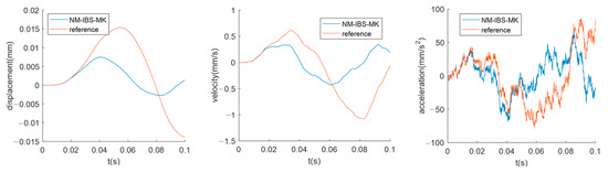
Figure 8. The incorrect results when the force equilibrium is not satisfied.

The coefficient $\alpha$ in Equation (64) is used to fit the model. Now, we set $h_c=85$, the R2 of the acceleration in the Z direction, with the varying $\alpha$, as shown in Table 3.

Table 3. R2 of acceleration between the NMI-IBS and the reference in Z direction with various $\alpha$.

$\mathit{\alpha }$	0.25	0.5	1	2	4
NMI-IBS-MK	0.96434	0.96685	0.97903	0.98816	0.91627
NMI-IBS-MSL	0.98576	0.98563	0.98491	0.98494	0.98646

The results in Table 3 show that the performance of the moving Kriging interpolation scheme is more sensitive with $\alpha$. However, as shown in Table 2 and Table 3, both interpolation schemes perform well enough when $\alpha$ and $h_c$ remain within an appropriate range. In practice, $\alpha$ and $h_c$ can be selected empirically by considering the configuration of the interfaces.

Finally, to implement the assembly of multi-domain substructure methods, the results of the assembly of IBS-IBS, IBS-FEM and IBS-CMS are compared in Configuration 1 with moving Kriging interpolation functions. Under the configuration of the interface support nodes with $h_c=85$ and $\alpha =1$, the analysis results in the Z direction are compared in Figure 9.

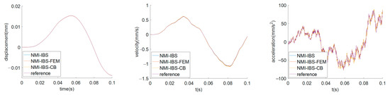
Figure 9. Comparison between the NMI-IBS, NMI-IBS-FEM, NMI-IBS-CB and the reference for the solid plate.

The result shows that the proposed method performs excellently for the dynamics of multi-domain substructures with non-matching interfaces and that there are only slight differences between IBS and IBS-FEM. The R2 and RAAE of the three methods are listed in Table 4.

Table 4. Accuracy of the multi-domain assembly for the solid plate under Configuration 1.

	R2		RAAE
	NMI-IBS	NMI-IBS-FEM	NMI-IBS	NMI-IBS-FEM
Displacement	0.99984	0.99971	0.00942	0.01367
Velocity	0.99963	0.99955	0.01121	0.01567
Acceleration	0.97822	0.97885	0.10453	0.10514

Ultimately, both of the interpolation schemes satisfy the basic rule of the normalization condition and show good performance in dynamic response prediction. The examples illustrate that the proposed method is accurate and efficient in the dynamic response prediction of substructure IRFs with non-matching interfaces.

5.2. Application to Lunar Lander with a Rover

We analyzed the dynamic response of the lunar lander landing process to validate the method; the FEM model is shown in Figure 9. The main components of the lander include: (1) the center body, (2) the payloads and auxiliary equipment and (3) the landing mechanism.

In this example, we only retained the main body, the solar wings and the rover. Other payloads are simplified as the distributed inertia, which adheres to the original position.

The rover attaches to the main body of the lunar lander when it is transported to the moon. When arriving at the destination, it separates from the main body and starts cruising, becoming an independent system.

Usually, the rover and the center body of the lander are developed by different branches separately during the prototype design process. Moreover, the development process of the rover is an iterative optimization process, and during every iteration, the modified rover should be assembled with the center body for coupling analysis. So, we used a modal substructure to model it.

However, the center body and the rover usually have non-matched node distributions on the interface since their FE models are established by different design groups, as shown in Figure 10 (right). Moreover, there are some complex connecting relations inside the center body and the rover that are commonly based on nodes. Consequently, remeshing will lead to an enormous cost for rebuilding those connecting relations. Therefore, the non-matching interface method is suitable in this case.

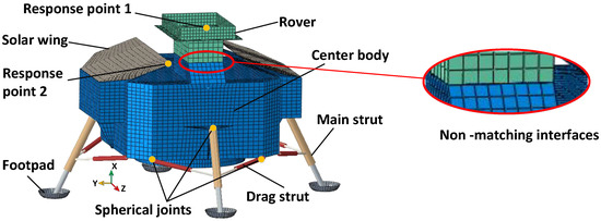
Figure 10. Finite element model of the lunar lander coupled with a rover by non-matching interfaces.

In this example, the lunar lander contains two types of substructures (the center body with solar wings is an IBS substructure and the rover is an FE substructure), and the method of initial applied forces with the Newmark-$\beta$ scheme is used to compute the approximate IRFs.

There are 40 support nodes selected on the rover interface and 34 support nodes on the center body interface. The intermediate surface coincides with the rover interface, shown in Figure 11, and with the coefficient $\alpha =1$ and $h_c=0.5$ (referring to the size of the interface), the interpolation functions are generated.

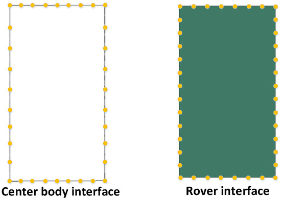
Figure 11. Distribution of interface support nodes on rover and center body.

According to Chen [15], we obtain the buffer loads acting on the center body. Take the longitudinal (X direction) buffer load generated from the Z-direction main strut, for instance [13]; its time history is shown in Figure 12.

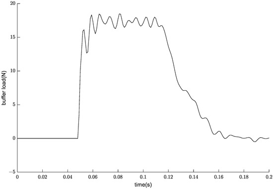
Figure 12. Longitudinal buffer load [13].

There are two response points (see Figure 10) selected on the lunar lander: Point 1 is on the rover and Point 2 is on the left solar wing. Using the proposed NMI-IBS, NMI-IBS-FEM and NMI-IBS-CB (all modes retained), the acceleration responses of the response points are computed. To illustrate the accuracy of these methods, an FE model with the coinciding interface is given as the reference, and the dynamic responses are obtained under the same conditions: gravity ($g=1.63 \mathrm{m}/{\mathrm{s}}^2$) and initial vertical landing velocity ($v=4 \mathrm{m}/\mathrm{s}$). The results are shown in Figure 13.

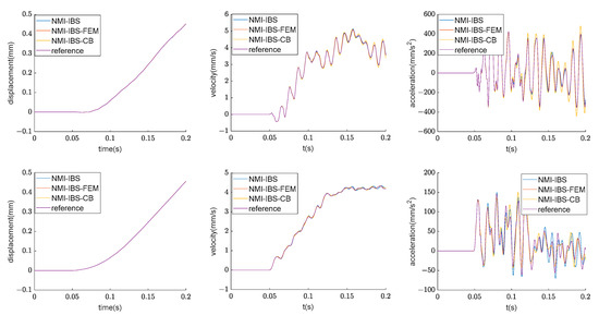
Figure 13. Comparison among NMI-IBS, NMI-IBS-FEM, NMI-IBS-CB (all modes retained) and the reference for the lunar lander (down for the response point 1 and up for the response point 2).

To make a clear comparison of the accuracy, R2 is listed in Table 5.

Table 5. Accuracy of the NMI-IBS for responses of the lunar lander in X direction.

	Response Point 1			Response Point 2
	NMI-IBS	NMI-IBS-FEM	NMI-IBS-CB	NMI-IBS	NMI-IBS-FEM	NMI-IBS-CB
Displacement	1.00000	1.00000	1.00000	1.00000	1.00000	1.00000
Velocity	0.99978	0.99986	0.99985	0.99988	0.99893	0.99887
Acceleration	0.90056	0.89039	0.89039	0.99466	0.94777	0.94774

These results show that displacement and velocity have strong agreement with the reference at both of the two response points. Meanwhile, the acceleration result has a relatively high accuracy performance.

Moreover, when the IRFs of the substructures are known, the total CPU times of NMI-IBS, NMI-IBS-FEM and full Newmark-β time integration are 38.63 s, 173.96 s and 2685 s, respectively, under the same computer hardware conditions (CPU: Intel Core i5-2300, RAM: 8 GB), shown in Table 6. The most time-consuming process for the NMI-IBS is the calculation of IRFs. However, in practice, this preparation time for the IRFs can be reduced because the columns of the IRF matrix can be calculated simultaneously and the calculation is applicable to all. When facing design optimization or multiple load cases, by using NMI-IBS, efficiency can be drastically improved. NMI-IBS-FEM takes more time than NMI-IBS, but it could still improve the calculation efficiency. Moreover, these two methods do not need to calculate IRFs in advance, which might be more efficient than NMIS-IBS when the number of cases is not too large.

Table 6. CPU time used for responses of the lunar lander.

	NMI-IBS	NMI-IBS-FEM	NMI-IBS-CB	Full Newmark-β
CPU time	38.63 s	173.96 s	158.87	2685 s

This example shows that the multi-domain substructure methods can manage the practical assembly of substructures with non-matching interfaces conveniently and efficiently, with high accuracy.

6. Conclusions

This paper extends the ordinary IBS method and presents a method for coupling multi-domain substructures, including IBS, FEM and modal substructures, with non-matching interfaces. The method has engineering application value. The following conclusions are drawn:

(1)

A method for assembling multi-domain substructures with non-matching interfaces is proposed in this paper. It is an extension of the available IBS techniques and makes the IBS method more practical for coupling multi-domain substructures. Like the original IBS, this method can deal with complex dynamics efficiently.

(2)

The basic rule of generating the interpolation functions is discussed, and by achieving the normalization condition, force equilibrium and energy conservation can be conveniently satisfied. Compared with the approach of constructing transition elements, it is unnecessary to implement a complicated element construction process; only the distribution of support nodes and the coefficients are needed, and a different model can be used for interpolation functions when it satisfies the normalization condition.

(3)

The advantageous performance of this method in dynamic prediction is validated by two numerical examples: one is the dynamic simulation of the landing process of a lunar lander. With high accuracy, the time-consuming simulation of the landing process is drastically reduced by the employment of the proposed method.

(4)

Not all mesh grid points on interfaces are needed, and the support nodes can be selected properly considering the features of the interfaces and the engineering accuracy requirements. A more rigorous study about the support node selection considering their precise influence will be further studied as an alternative reduction of the interfaces.

References

- Hurty, W.C. Vibrations of structural systems by component mode synthesis. J. Eng. Mech. Div. 1960, 86, 51–70. [Google Scholar] [CrossRef]
- Craig, R.R., Jr. Coupling of substructures for dynamic analyses: An overview. In Proceedings of the 41st AIAA/ASME/ASCE/AHS/ASC Structures, Structural Dynamics, and Materials Conference and Exhibit, Atlanta, GA, USA, 3–6 April 2000; AIAA Paper 2000-1573. The University of Texas: Austin, TX, USA, 2000. [Google Scholar]
- Jetmundsen, B.; Bielawa, R.L.; Flannelly, W.G. Generalized frequency domain substructure synthesis. J. Am. Helicopter Soc. 1988, 33, 55–64. [Google Scholar] [CrossRef]
- Rixen, D.J.; van der Valk, P.L.C. An Impulse Based Substructuring approach for impact analysis and load case simulations. J. Sound Vib. 2013, 332, 7174–7190. [Google Scholar] [CrossRef]
- De Klerk, D.; Rixen, D.J.; Voormeeren, S.N. General framework for dynamic substructuring: History, review, and classification of techniques. AIAA J. 2008, 46, 1169–1181. [Google Scholar] [CrossRef]
- Rixen, D.; Haghighat, N. Truncating the Impulse Responses of Substructures to Speed Up the Impulse-Based Substructuring. In Proceedings of the 30th International Modal Analysis Conference, Jacksonville, FL, USA, 1–4 February 2012; Springer: New York, NY, USA, 2012; Volume 2, pp. 137–148. [Google Scholar] [CrossRef]
- Gordis, J.H. Integral equation formulation for transient structural synthesis. AIAA J. 1995, 33, 320–324. [Google Scholar] [CrossRef]
- Rixen, D.J. Substructuring Using Impulse Response Functions for Impact Analysis. In Proceedings of the 28th International Modal Analysis Conference, Jacksonville, FL, USA, 1–4 February 2010; Springer: New York, NY, USA, 2010; Volume 3, pp. 637–646. [Google Scholar]
- Rixen, D.J. A Substructuring Technique Based on Measured and Computed Impulse Response Functions of Components. In Proceedings of the Isma2010—International Conference on Noise and Vibration Engineering, KU Leuven, Leuven, Belgium, 20–22 September 2010; pp. 1939–1954. [Google Scholar]
- Van der Seijs, M.V.; Rixen, D.J. Efficient impulse based substructuring using truncated impulse response functions and mode superposition. In Proceedings of the International Conference on Noise and Vibration Engineering, KU Leuven, Leuven, Belgium, 14–15 September 2012; pp. 3487–3499. [Google Scholar]
- Van der Valk, P.L.C.; Rixen, D.J. An Effective Method for Assembling Impulse Response Functions to Linear and Non-Linear Finite Element Models. In Proceedings of the 30th International Modal Analysis Conference, Jacksonville, FL, USA, 1–4 February 2012; Springer: New York, NY, USA, 2012; Volume 2, pp. 123–135. [Google Scholar]
- Van der Valk, P.L.C.; Rixen, D.J. An Impulse Based Substructuring method for coupling impulse response functions and finite element models. Comput. Methods Appl. Mech. Eng. 2014, 275, 113–137. [Google Scholar] [CrossRef]
- Dong, W.-L.; Liu, L.; Zhou, S.-D.; Chen, S.-L. Substructure Synthesis in Time Domain with Rigid-Elastic Hybrid Joints. AIAA J. 2015, 53, 504–509. [Google Scholar] [CrossRef]
- Zhou, S.-D.; Liu, L.; Dong, W.-L. Time-Domain Substructure Synthesis with Hybrid Rigid and Nonlinear-Elastic Joints. AIAA J. 2016, 54, 2545–2551. [Google Scholar] [CrossRef]
- Chen, S.; Liu, L.; Zhou, S.; Chen, Z.; Yue, Z. Multi-domain substructures synthesis with general joints for the dynamics of large structures. AIP Adv. 2017, 7, 105007. [Google Scholar] [CrossRef]
- Aminpour, M.; Ransom, J.; McCleary, S. Coupled analysis of independently modeled finite element subdomains. In Proceedings of the 33rd Structures, Structural Dynamics and Materials Conference, Dallas, TX, USA, 13–15 April 1992; pp. 109–120. [Google Scholar] [CrossRef]
- Aminpour, M.; Pageau, S.; Shin, Y. Improved interface modeling technology. In Proceedings of the 19th AIAA Applied Aerodynamics Conference, Anaheim, CA, USA, 11–14 June 2001; p. 1548. [Google Scholar] [CrossRef]
- Ransom, J.; McCleary, S.; Aminpour, M. A New Interface Element for Connecting Independently Modeled Substructures. In Proceedings of the 34th Structures, Structural Dynamics and Materials Conference, La Jolla, CA, USA, 19–22 April 1993; p. 1503. [Google Scholar]
- Park, K.C.; Felippa, C.A. A variational principle for the formulation of partitioned structural systems. Int. J. Numer. Methods Eng. 2000, 47, 395–418. [Google Scholar] [CrossRef]
- Bfer, G. An Isoparametric Joint Interface Element for Finite-Element Analysis. Int. J. Numer. Methods Eng. 1985, 21, 585–600. [Google Scholar] [CrossRef]
- Gens, A.; Carol, I.; Alonso, E.E. An interface element formulation for the analysis of soil-reinforcement interaction. Comput. Geotech. 1989, 7, 133–151. [Google Scholar] [CrossRef]
- Dávila, C.G. Solid-To-Shell Transition-Elements for the Computation of Interlaminar Stresses. Comput. Syst. Eng. 1994, 5, 193–202. [Google Scholar] [CrossRef]
- Kim, H.G. Interface element method (IEM) for a partitioned system with non-matching interfaces. Comput. Methods Appl. Mech. Eng. 2002, 191, 3165–3194. [Google Scholar] [CrossRef]
- Cho, Y.-S.; Jun, S.; Im, S.; Kim, H.-G. An improved interface element with variable nodes for non-matching finite element meshes. Comput. Methods Appl. Mech. Eng. 2005, 194, 3022–3046. [Google Scholar] [CrossRef]
- Cho, J.Y.; An, J.; Jee, Y.B. Displacement Welding Technique for Coupled Analysis of Independently Modeled Finite Element Substructures. In Proceedings of the 44th AIAA/ASME/ASCE/AHS Structures, Structural Dynamics, and Materials Conference, Norfolk, VA, USA, 7–10 April 2003; p. 1677. [Google Scholar] [CrossRef]
- De Boer, A.; van Zuijlen, A.; Bijl, H. Review of coupling methods for non-matching meshes. Comput. Methods Appl. Mech. Eng. 2007, 196, 1515–1525. [Google Scholar] [CrossRef]
- Oliver, M.A.; Webster, R. Kriging: A method of interpolation for geographical information systems. Int. J. Geogr. Inf. Syst. 1990, 4, 313–332. [Google Scholar] [CrossRef]
- Jin, R.; Chen, W.; Simpson, T.W. Comparative studies of metamodelling techniques under multiple modelling criteria. Struct. Multidiscip. Optim. 2001, 23, 1–13. [Google Scholar] [CrossRef]
- Dai, K.Y.; Liu, G.R.; Lim, K.M.; Gu, Y.T. Comparison between the radial point interpolation and the Kriging interpolation used in meshfree methods. Comput. Mech. 2003, 32, 60–70. [Google Scholar] [CrossRef]
- Chassaing, J.-C.; Nogueira, X.; Khelladi, S. Moving Kriging reconstruction for high-order finite volume computation of compressible flows. Comput. Methods Appl. Mech. Eng. 2013, 253, 463–478. [Google Scholar] [CrossRef]
- Gu, L. Moving kriging interpolation and element-free Galerkin method. Int. J. Numer. Methods Eng. 2003, 56, 1–11. [Google Scholar] [CrossRef]
- Pian, T.H.H.; Tong, P. Basis of finite element methods for solid continua. Int. J. Numer. Methods Eng. 1969, 1, 3–28. [Google Scholar] [CrossRef]
- Belytschko, T.; Organ, D.; Krongauz, Y. A coupled finite element-element-free Galerkin method. Comput. Mech. 1995, 3, 186–195. [Google Scholar] [CrossRef]
Disclaimer/Publisher’s Note: The statements, opinions and data contained in all publications are solely those of the individual author(s) and contributor(s) and not of MDPI and/or the editor(s). MDPI and/or the editor(s) disclaim responsibility for any injury to people or property resulting from any ideas, methods, instructions or products referred to in the content. |
© 2023 by the authors. Licensee MDPI, Basel, Switzerland. This article is an open access article distributed under the terms and conditions of the Creative Commons Attribution (CC BY) license (https://creativecommons.org/licenses/by/4.0/).