
State-of-Charge Prediction Model for Ni-Cd Batteries Considering Temperature and Noise

Abstract
1. Introduction
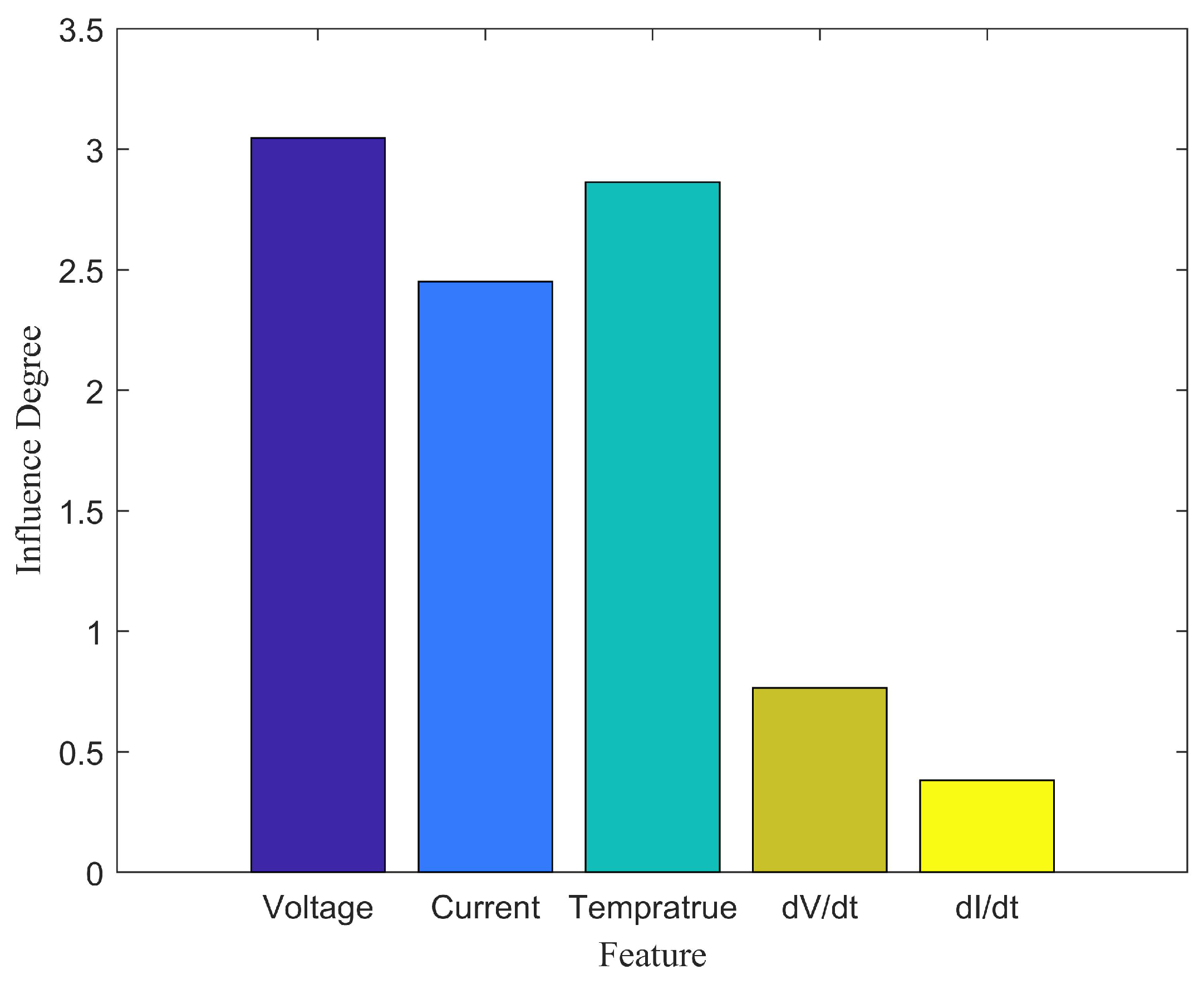
2. Optimal Feature Selection
3. APSO-GRNN Algorithm
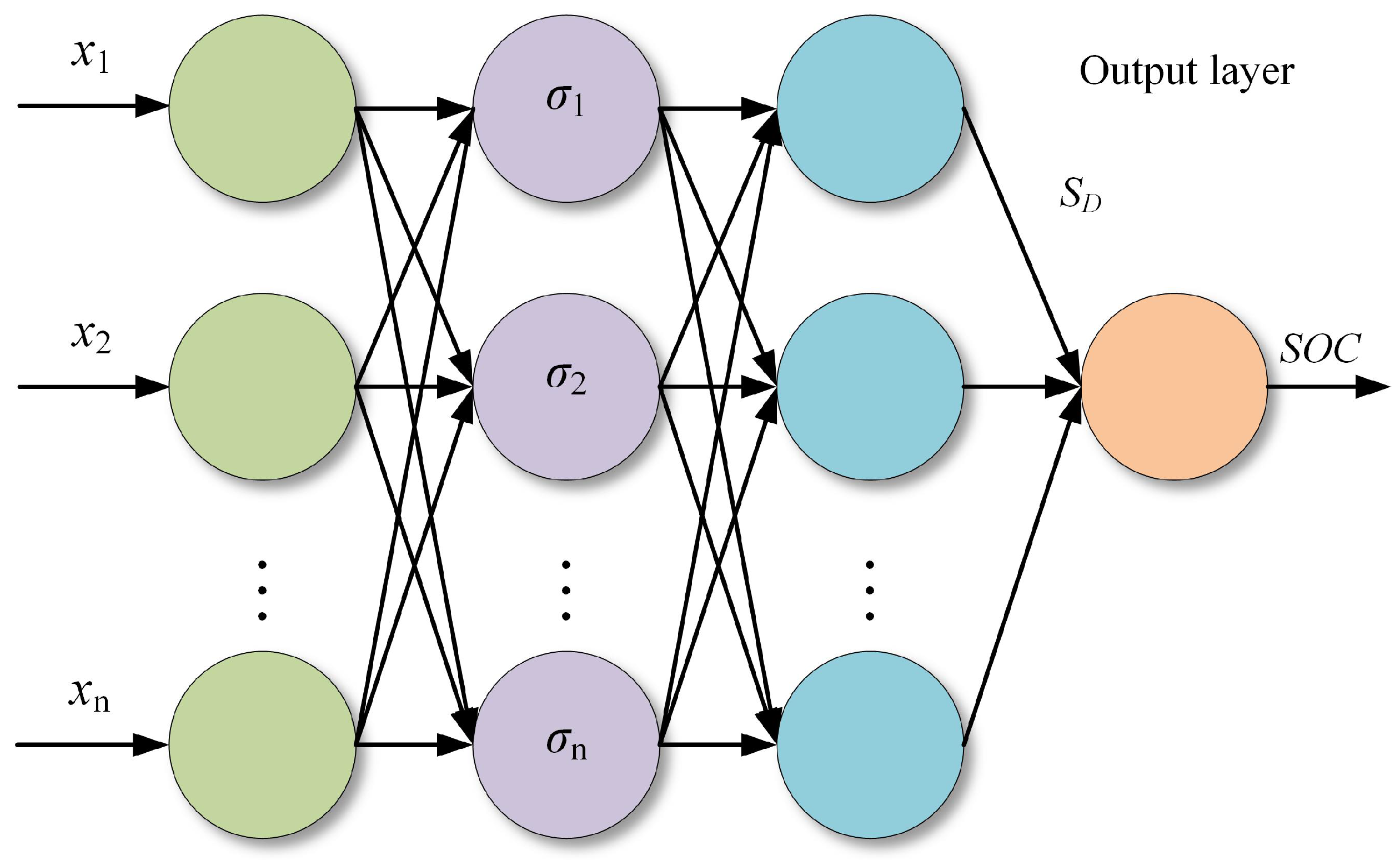
3.1. The GRNN Model
- Input layerThe number of neurons in the input layer is equal to the vector dimension of the sample dataset, and each neuron in the input layer is equivalent to an identical function, which directly passes the input variable to the pattern layer.
- Pattern layerThe pattern layer is fully connected and the number of neurons is set to the total number of training samples n. Each neuron corresponds to a different training sample. The value of the Gassu function for any training sample and test sample is shown in Equation (2).where is the model smoothing factor.
- Summation layerThe number of neurons in the summation layer is one more than the sample dimension. The summation layer has two outputs: the first neuron output is the summation of the pattern layer outputs. For any summation layer neuron with inputs , the transfer function for the first summation layer neuron is as follows:The remaining neuron outputs are the weighted sum of the pattern layer outputs, with a transfer function as follows:where is the corresponding eigenvalue of any training sample.
- Output layer
3.2. Optimization Process of APSO Algorithm
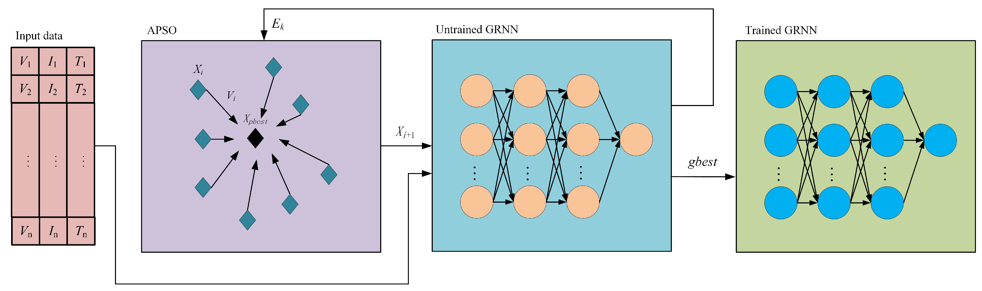
3.3. Prediction Process of Battery SOC Based on APSO-GRNN Model
- Initialize the particle swarm algorithm parameters. The initial particle population size is m × n, where m is the number of particle vectors, n is the number of neurons in the summation layer, and the number of iterations is T. The smoothing factor of each neuron in the summation layer is taken as the position attribute of the particle , and the particle position parameters and matrix parameters are randomly initialized.
- Assuming that the GRNN model is a fitness calculation model, the error matrix of the particle swarm is calculated using Equations (9) and (13) as e, and the error vector of a single particle is .
- The local optimal value and each particle’s global optimal value are updated according to the error matrix. The particle swarm velocity weight matrix w is modified using Equation (13), and the particle swarm position vector and velocity vector are updated using Equations (7) and (8).
- Repeat Steps 2 and 3 until the error of the global optimal particle is less than the target error or the maximum number of iterations and then end the iteration. The algorithm’s structure is shown in Figure 3.
4. Analysis of SOC Prediction Results of Ni-Cd Battery Using APSO-GRNN
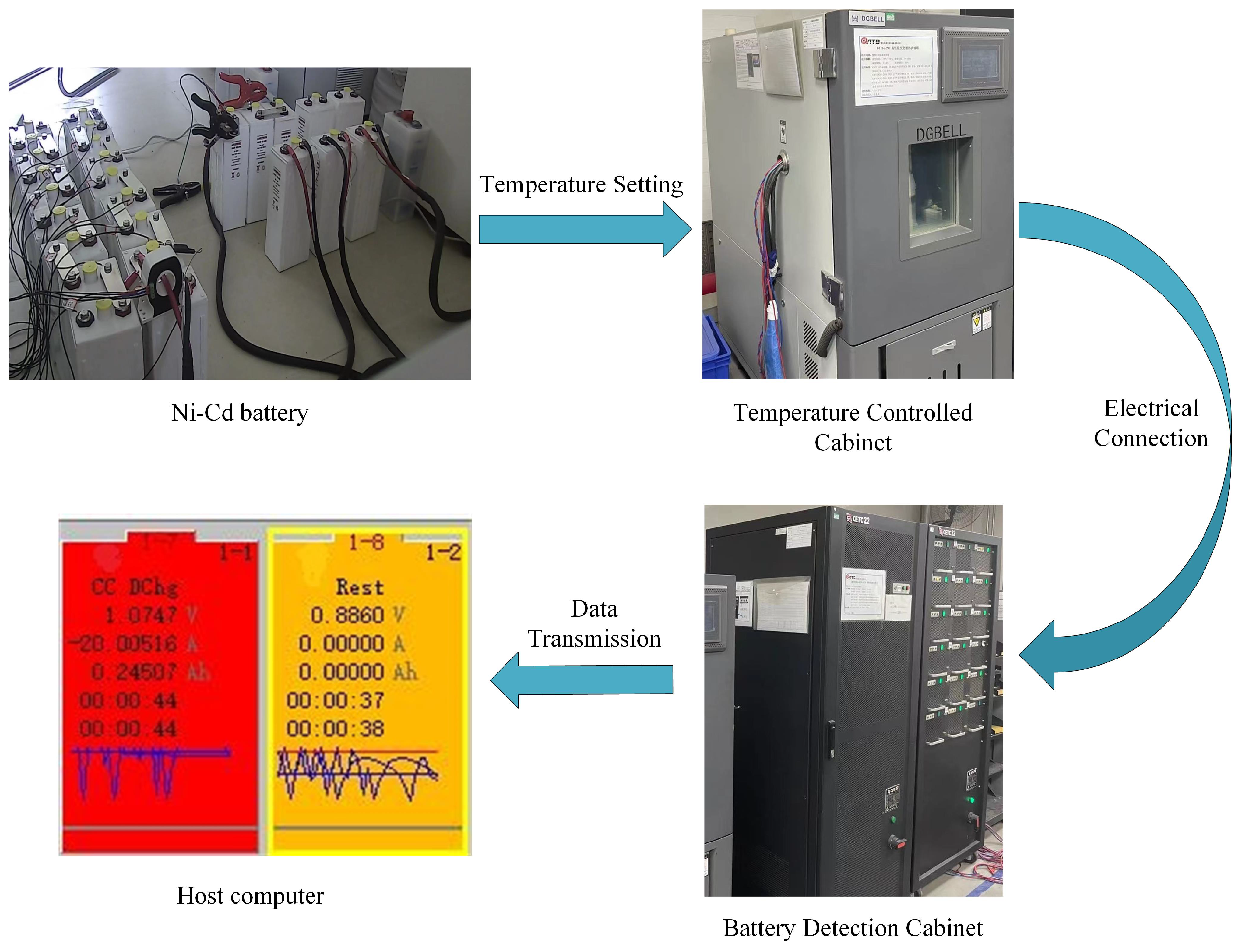
4.1. Test Platform and Experimental Method
4.2. SOC Prediction Algorithm Results and Discussion
4.2.1. APSO-GRNN Model Training Results
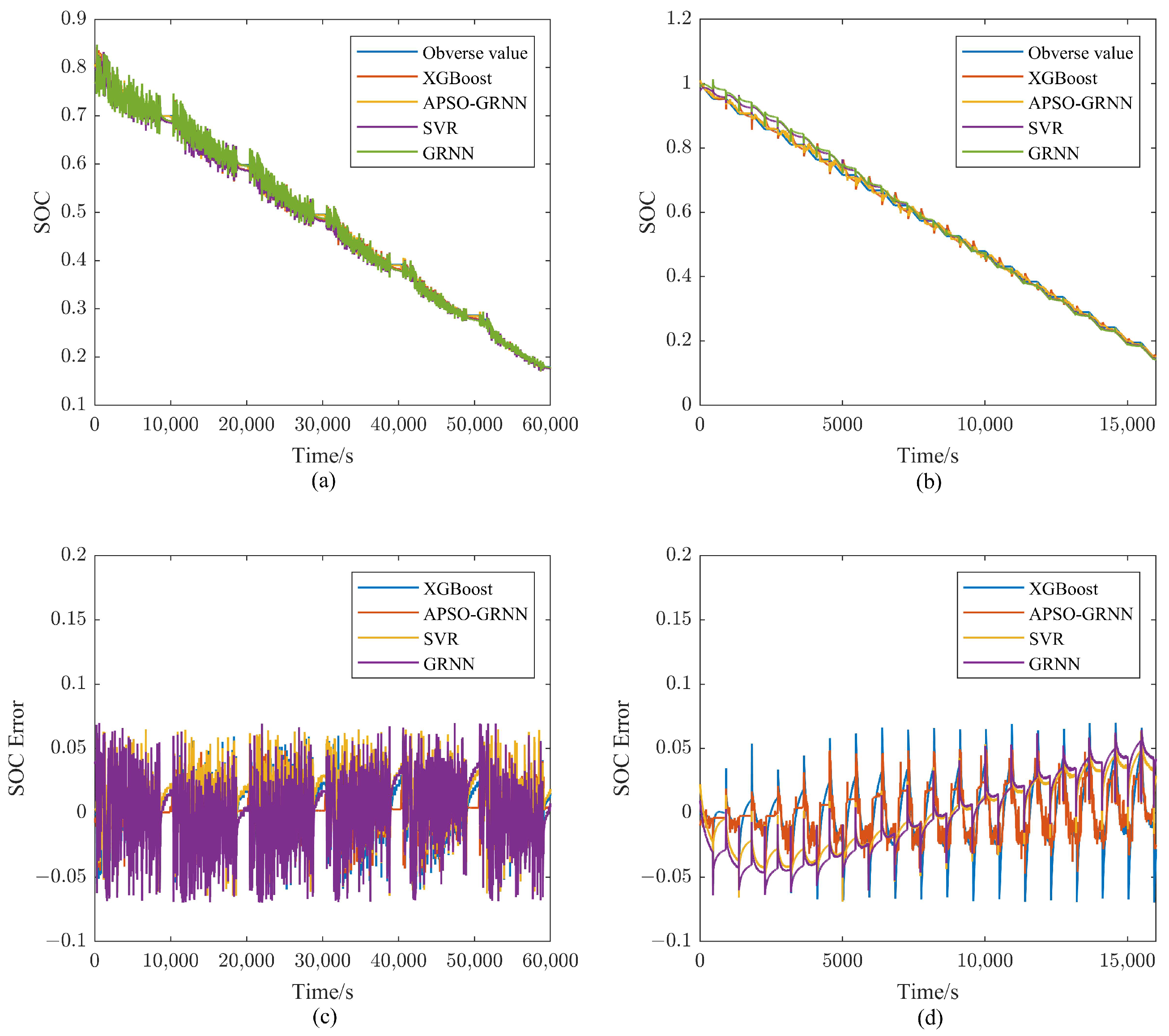
4.2.2. Model Robustness Test Results for Noise
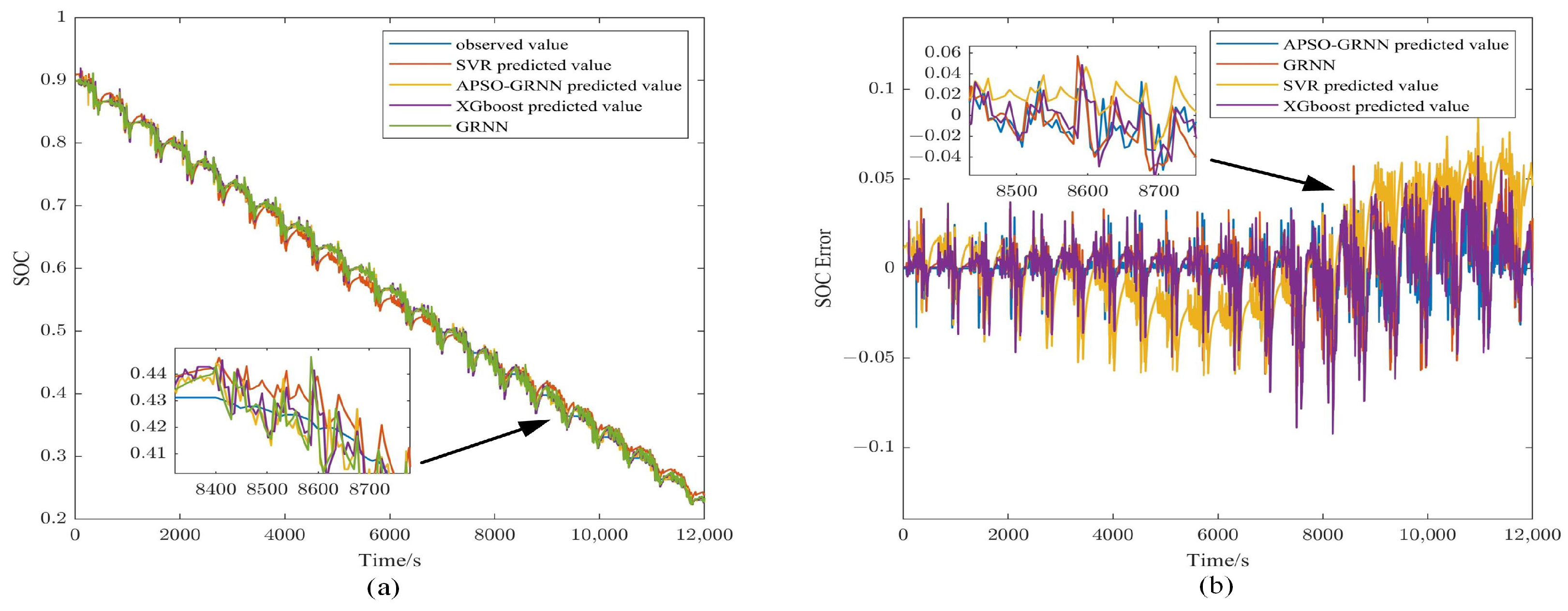
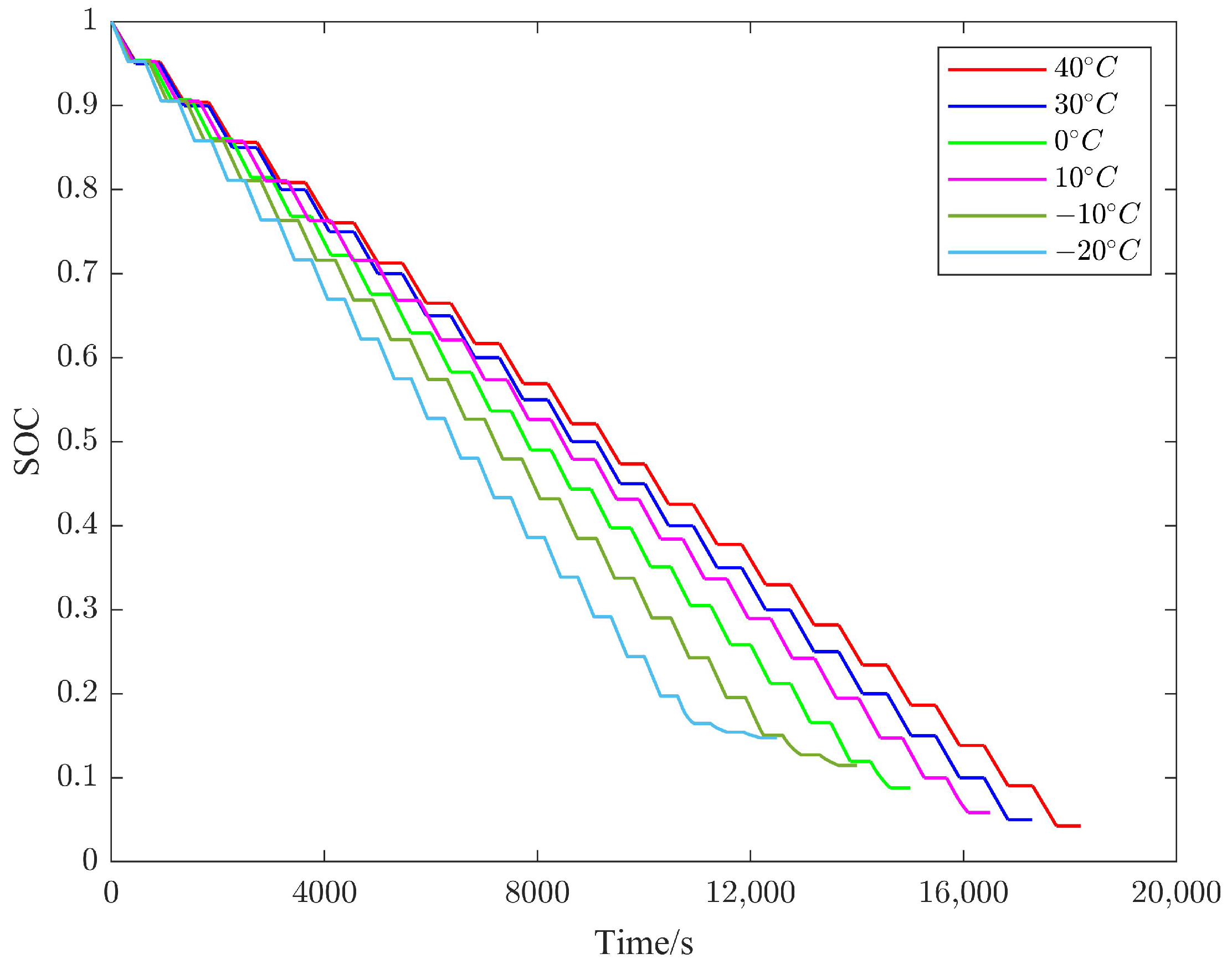
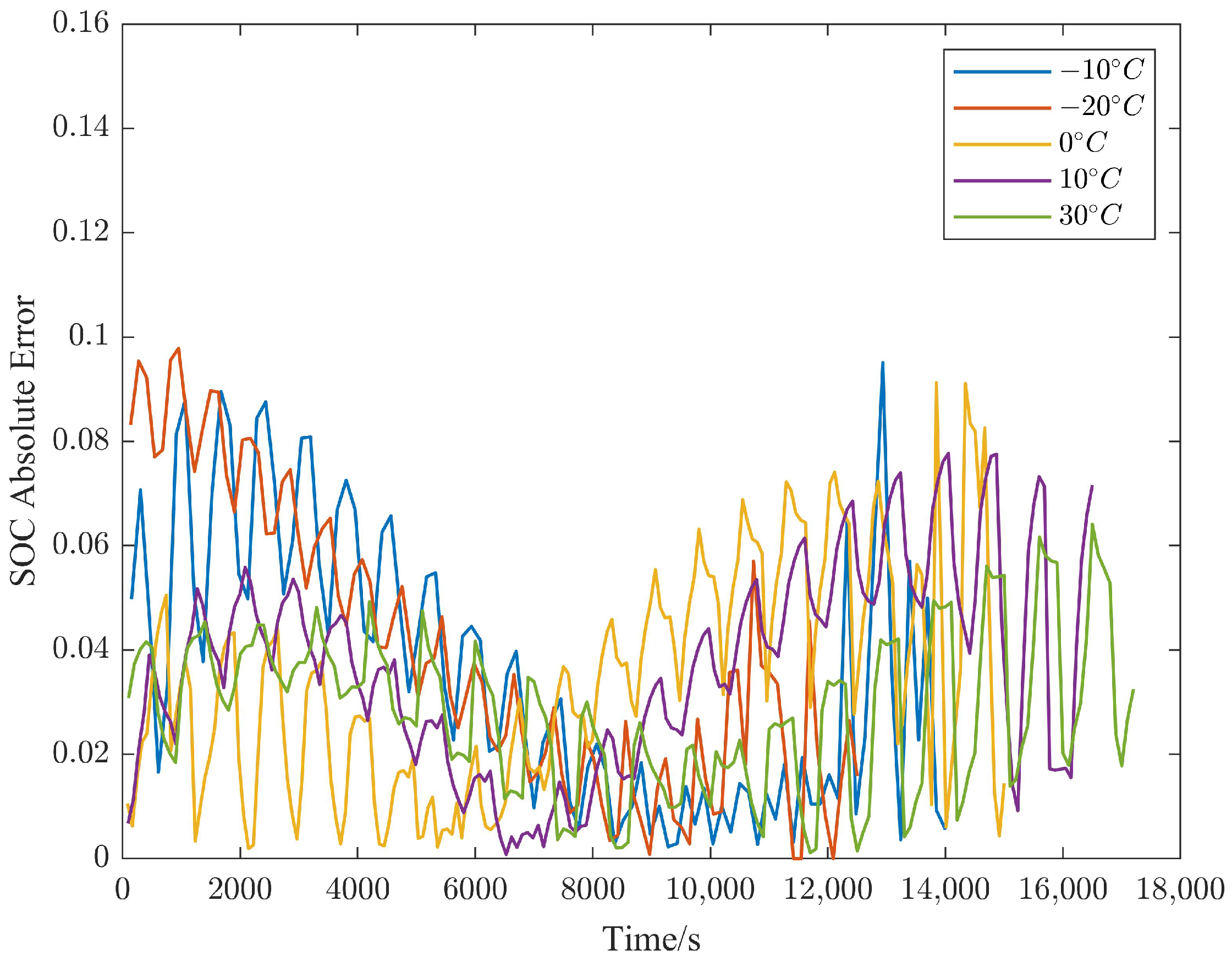
4.2.3. Model Robustness Test Results for Temperature
5. Conclusions
- The advantages and disadvantages of SOC prediction models proposed in the literature were analyzed, and a GRNN model with adaptive adjustment was proposed based on the characteristics of nickel-cadmium batteries. This contribution enriches the research methods for the SOC prediction of nickel-cadmium batteries and provides a new theoretical reference for developing energy management strategies for train battery packs.
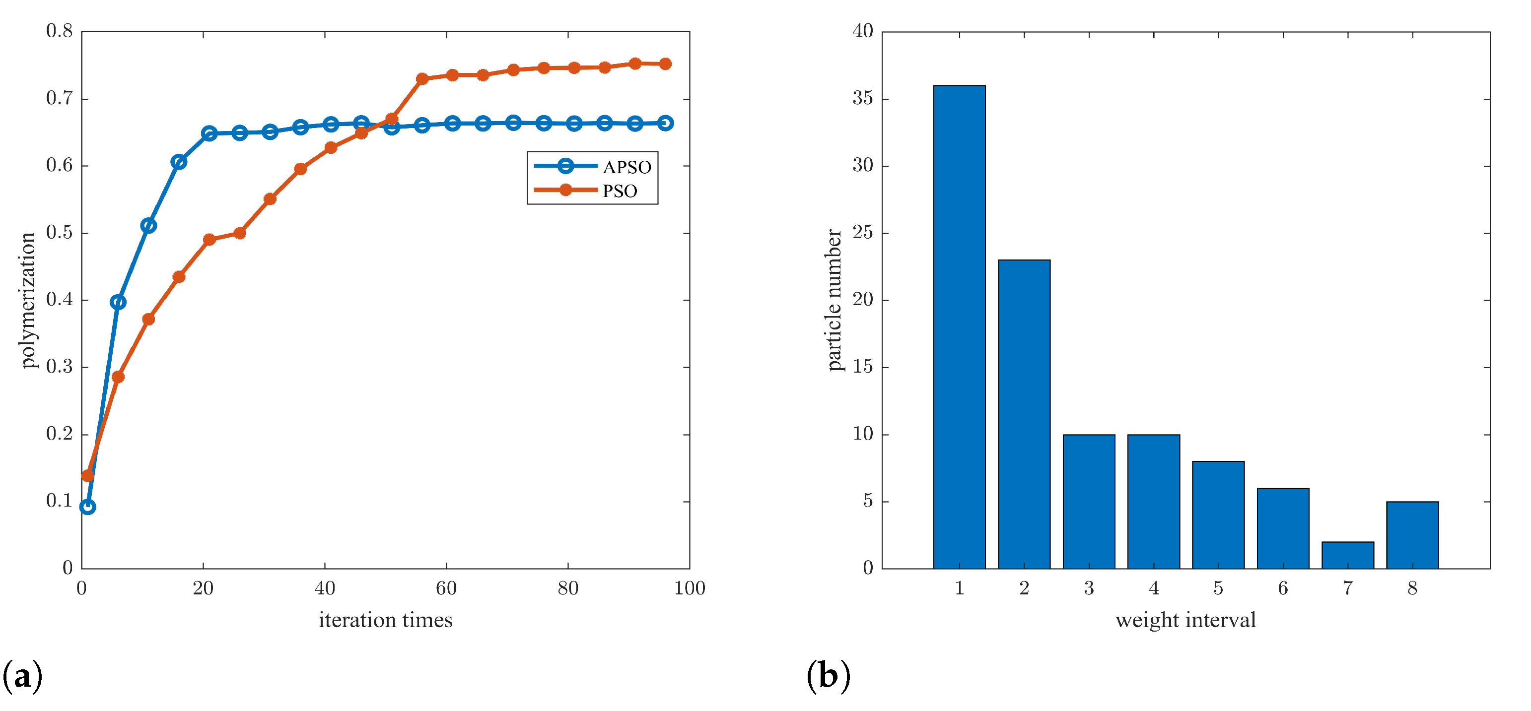
- A comparison of the prediction results of the APSO-GRNN and GRNN models showed that APSO can enhance the diversity of mode-layer smoothing factors and improve the accuracy of SOC prediction. It was demonstrated that APSO can filter the time series and adjust the size of each neuron smoothing factor based on the correlation of the time series. Thus, the model prioritizes historical data that has a more significant impact on the current moment.
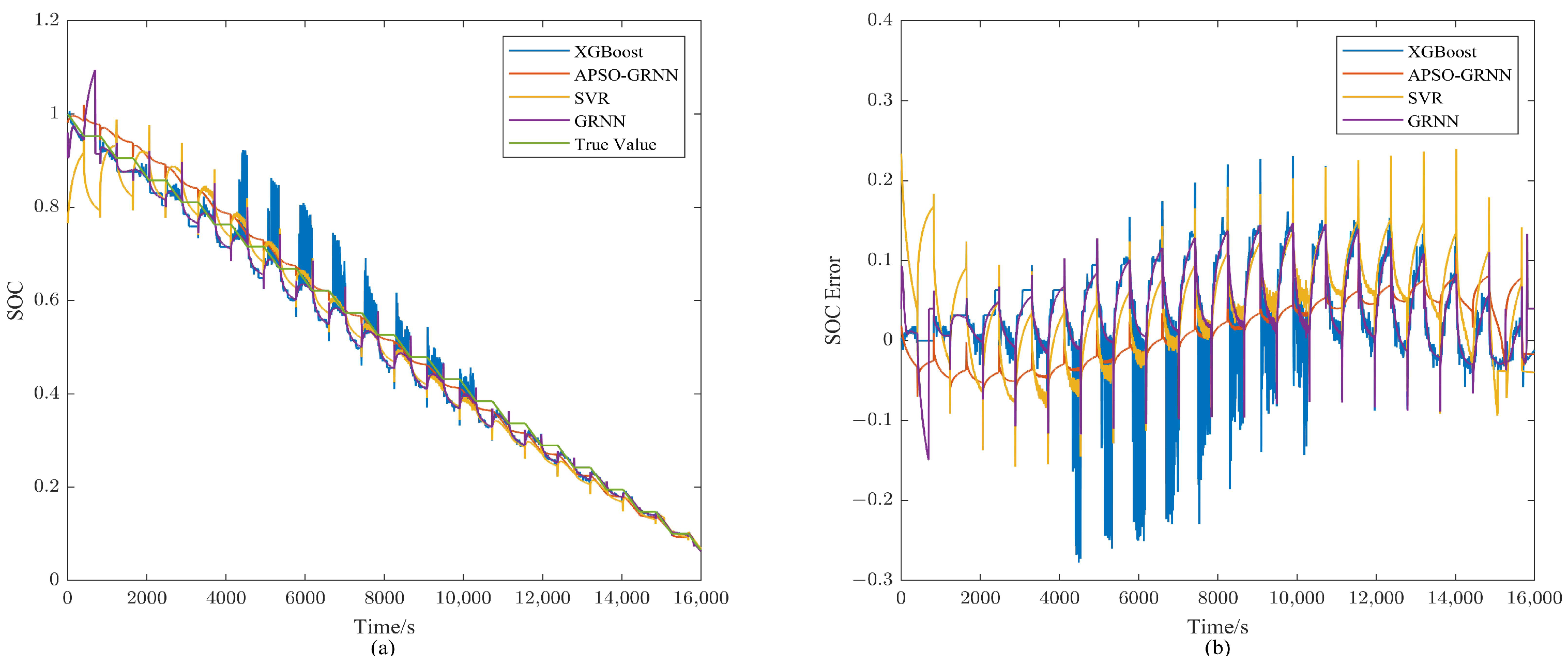
- Two experimental scenarios were designed to verify the robustness of the APSO-GRNN model against noise interference and temperature changes. The prediction results were compared with those of the GRNN, SVR, and XGBoost models. The experimental results demonstrated that the APSO-GRNN model can maintain a high prediction accuracy, even under changing experimental conditions, temperatures, and noise interference.
- The APSO-GRNN model is suitable for the online prediction of the SOC of nickel-cadmium batteries due to its reduced number of parameters, shorter training time, and stronger real-time performance. It can be deployed in an onboard battery management system (BMS) to provide a theoretical basis for battery energy management strategies. In future research, we plan to broaden the scope of this study by incorporating real-world applications of train Ni-Cd batteries.
Author Contributions
Funding
Institutional Review Board Statement
Informed Consent Statement
Data Availability Statement
Conflicts of Interest
Nomenclature
| F | Multidisciplinary Digital Publishing Institute. |
| The out-of-bag error after random rearrangement of the feature . | |
| The error of the sample in the decision tree T. | |
| The i-th training sample. | |
| The j-th testing sample. | |
| The model smoothing factor. | |
| The output of the i-th pattern layer neuron. | |
| The corresponding eigenvalue of any training sample. | |
| The position vector of the particle. | |
| The velocity vector of the particle. | |
| The historical optimal value of the particle. | |
| The group optimal value in the current particle population. | |
| The true value of the training set. | |
| The prediction error matrix of the k-th iteration of the model. | |
| h | The error score matrix. |
| The error threshold that the particle swarm should reach to stop the iteration. | |
| The prediction error of the global optimal particle. | |
| The average optimal fitness of all particles in the current epoch. |
References
- Espedal, I.B.; Jinasena, A.; Burheim, O.S.; Lamb, J.J. Current trends for state-of-charge (SoC) estimation in lithium-ion battery electric vehicles. Energies 2021, 14, 3284. [Google Scholar] [CrossRef]
- Wang, Y.; Tian, J.; Sun, Z.; Wang, L.; Xu, R.; Li, M.; Chen, Z. A comprehensive review of battery modeling and state estimation approaches for advanced battery management systems. Renew. Sustain. Energy Rev. 2020, 131, 110015. [Google Scholar] [CrossRef]
- Wang, H.; Zhou, G.; Xu, J.; Liu, Z.; Yan, X.; McCann, J.A. A Simplified Historical-Information-Based SOC Prediction Method for Supercapacitors. IEEE Trans. Ind. Electron. 2021, 69, 13090–13098. [Google Scholar] [CrossRef]
- Wu, X.; Li, M.; Du, J.; Hu, F. SOC prediction method based on battery pack aging and consistency deviation of thermoelectric characteristics. Energy Rep. 2022, 8, 2262–2272. [Google Scholar] [CrossRef]
- Capizzi, G.; Bonanno, F.; Napoli, C. Hybrid neural networks architectures for SOC and voltage prediction of new generation batteries storage. In Proceedings of the 2011 International Conference on Clean Electrical Power (ICCEP), Ischia, Italy, 14–16 June 2011; pp. 341–344. [Google Scholar]
- Farmann, A.; Sauer, D.U. A comprehensive review of on-board State-of-Available-Power prediction techniques for lithium-ion batteries in electric vehicles. J. Power Sources 2016, 329, 123–137. [Google Scholar] [CrossRef]
- Zhao, X.; de Callafon, R.A. Modeling of battery dynamics and hysteresis for power delivery prediction and SOC estimation. Appl. Energy 2016, 180, 823–833. [Google Scholar] [CrossRef]
- Li, Y.; Xu, G.; Xu, B.; Zhang, Y. A novel fusion model for battery online state of charge (SOC) estimation. Int. J. Electrochem. Sci. 2021, 16, 4–15. [Google Scholar] [CrossRef]
- Green, A. The characteristics of the nickel-cadmium battery for energy storage. Power Eng. J. 1999, 13, 117–121. [Google Scholar] [CrossRef]
- McDowall, J. Nickel-cadmium batteries for energy storage applications. In Proceedings of the Fourteenth Annual Battery Conference on Applications and Advances. Proceedings of the Conference (Cat. No. 99TH8371), Long Beach, CA, USA, 12–15 January 1999; pp. 303–308. [Google Scholar]
- Zhang, S.; Guo, X.; Zhang, X. An improved adaptive unscented kalman filtering for state of charge online estimation of lithium-ion battery. J. Energy Storage 2020, 32, 101980. [Google Scholar] [CrossRef]
- Chen, L.; Tian, B.; Lin, W.; Ji, B.; Li, J.; Pan, H. Analysis and prediction of the discharge characteristics of the lithium–ion battery based on the Grey system theory. IET Power Electron. 2015, 8, 2361–2369. [Google Scholar] [CrossRef]
- Yan, W.; Zhang, B.; Zhao, G.; Tang, S.; Niu, G.; Wang, X. A battery management system with a Lebesgue-sampling-based extended Kalman filter. IEEE Trans. Ind. Electron. 2018, 66, 3227–3236. [Google Scholar] [CrossRef]
- Wang, J.; Zhang, L.; Mao, J.; Zhou, J.; Xu, D. Fractional order equivalent circuit model and SOC estimation of supercapacitors for use in HESS. IEEE Access 2019, 7, 52565–52572. [Google Scholar] [CrossRef]
- Hong, J.; Wang, Z.; Chen, W.; Wang, L.Y.; Qu, C. Online joint-prediction of multi-forward-step battery SOC using LSTM neural networks and multiple linear regression for real-world electric vehicles. J. Energy Storage 2020, 30, 101459. [Google Scholar] [CrossRef]
- Mao, X.; Song, S.; Ding, F. Optimal BP neural network algorithm for state of charge estimation of lithium-ion battery using PSO with Levy flight. J. Energy Storage 2022, 49, 104139. [Google Scholar] [CrossRef]
- Zhao, F.; Li, Y.; Wang, X.; Bai, L.; Liu, T. Lithium-ion batteries State of Charge prediction of electric vehicles using RNNs-CNNs neural networks. IEEE Access 2020, 8, 98168–98180. [Google Scholar] [CrossRef]
- Ren, L.; Dong, J.; Wang, X.; Meng, Z.; Zhao, L.; Deen, M.J. A data-driven auto-cnn-lstm prediction model for lithium-ion battery remaining useful life. IEEE Trans. Ind. Inform. 2020, 17, 3478–3487. [Google Scholar] [CrossRef]
- García-Plaza, M.; Serrano-Jiménez, D.; Carrasco, J.E.G.; Alonso-Martínez, J. A Ni–Cd battery model considering state of charge and hysteresis effects. J. Power Sources 2015, 275, 595–604. [Google Scholar] [CrossRef]
- Xuan, L.; Qian, L.; Chen, J.; Bai, X.; Wu, B. State-of-charge prediction of battery management system based on principal component analysis and improved support vector machine for regression. IEEE Access 2020, 8, 164693–164704. [Google Scholar] [CrossRef]
- Shen, Y. Adaptive online state-of-charge determination based on neuro-controller and neural network. Energy Convers. Manag. 2010, 51, 1093–1098. [Google Scholar] [CrossRef]
- Chen, T.; Xiao, L. Application of RBF and GRNN Neural Network Model in River Ecological Security Assessment—Taking the Middle and Small Rivers in Suzhou City as an Example. Sustainability 2023, 15, 6522. [Google Scholar] [CrossRef]
- Kulkarni, S.G.; Chaudhary, A.K.; Nandi, S.; Tambe, S.S.; Kulkarni, B.D. Modeling and monitoring of batch processes using principal component analysis (PCA) assisted generalized regression neural networks (GRNN). Biochem. Eng. J. 2004, 18, 193–210. [Google Scholar] [CrossRef]
- Rouhi, H.; Karola, E.; Serna-Guerrero, R.; Santasalo-Aarnio, A. Voltage behavior in lithium-ion batteries after electrochemical discharge and its implications on the safety of recycling processes. J. Energy Storage 2021, 35, 102323. [Google Scholar] [CrossRef]
- He, S.; Wu, J.; Wang, D.; He, X. Predictive modeling of groundwater nitrate pollution and evaluating its main impact factors using random forest. Chemosphere 2022, 290, 133388. [Google Scholar] [CrossRef]
- Speiser, J.L.; Miller, M.E.; Tooze, J.; Ip, E. A comparison of random forest variable selection methods for classification prediction modeling. Expert Syst. Appl. 2019, 134, 93–101. [Google Scholar] [CrossRef]
- Fei, H.; Fan, Z.; Wang, C.; Zhang, N.; Wang, T.; Chen, R.; Bai, T. Cotton classification method at the county scale based on multi-features and random forest feature selection algorithm and classifier. Remote Sens. 2022, 14, 829. [Google Scholar] [CrossRef]
- Wei, Z.; Leng, F.; He, Z.; Zhang, W.; Li, K. Online state of charge and state of health estimation for a Lithium-Ion battery based on a data–model fusion method. Energies 2018, 11, 1810. [Google Scholar] [CrossRef]
- Bao, H.; Yu, Y. State of charge estimation for electric vehicle batteries based on LS-SVM. In Proceedings of the 2013 5th International Conference on Intelligent Human-Machine Systems and Cybernetics, Hangzhou, China, 26–27 August 2013; Volume 1, pp. 442–445. [Google Scholar]
- Qiu, X.; Wu, W.; Wang, S. Remaining useful life prediction of lithium-ion battery based on improved cuckoo search particle filter and a novel state of charge estimation method. J. Power Sources 2020, 450, 227700. [Google Scholar] [CrossRef]
- Li, R.; Wang, H.; Dai, H.; Hong, J.; Tong, G.; Chen, X. Accurate state of charge prediction for real-world battery systems using a novel dual-dropout-based neural network. Energy 2022, 250, 123853. [Google Scholar] [CrossRef]
- Hussein, A.A. Experimental modeling and analysis of lithium-ion battery temperature dependence. In Proceedings of the 2015 IEEE Applied Power Electronics Conference and Exposition (APEC), Charlotte, NC, USA, 15–19 March 2015; pp. 1084–1088. [Google Scholar]


| Item | Parameter |
|---|---|
| Nominal capacity | 190 Ah |
| Initial weight | 6.1 kg |
| Initial voltage | 1.35 V |
| Resistance | |
| Initial density | 1.23 g/cm |
| Test Type | Experimental Process |
|---|---|
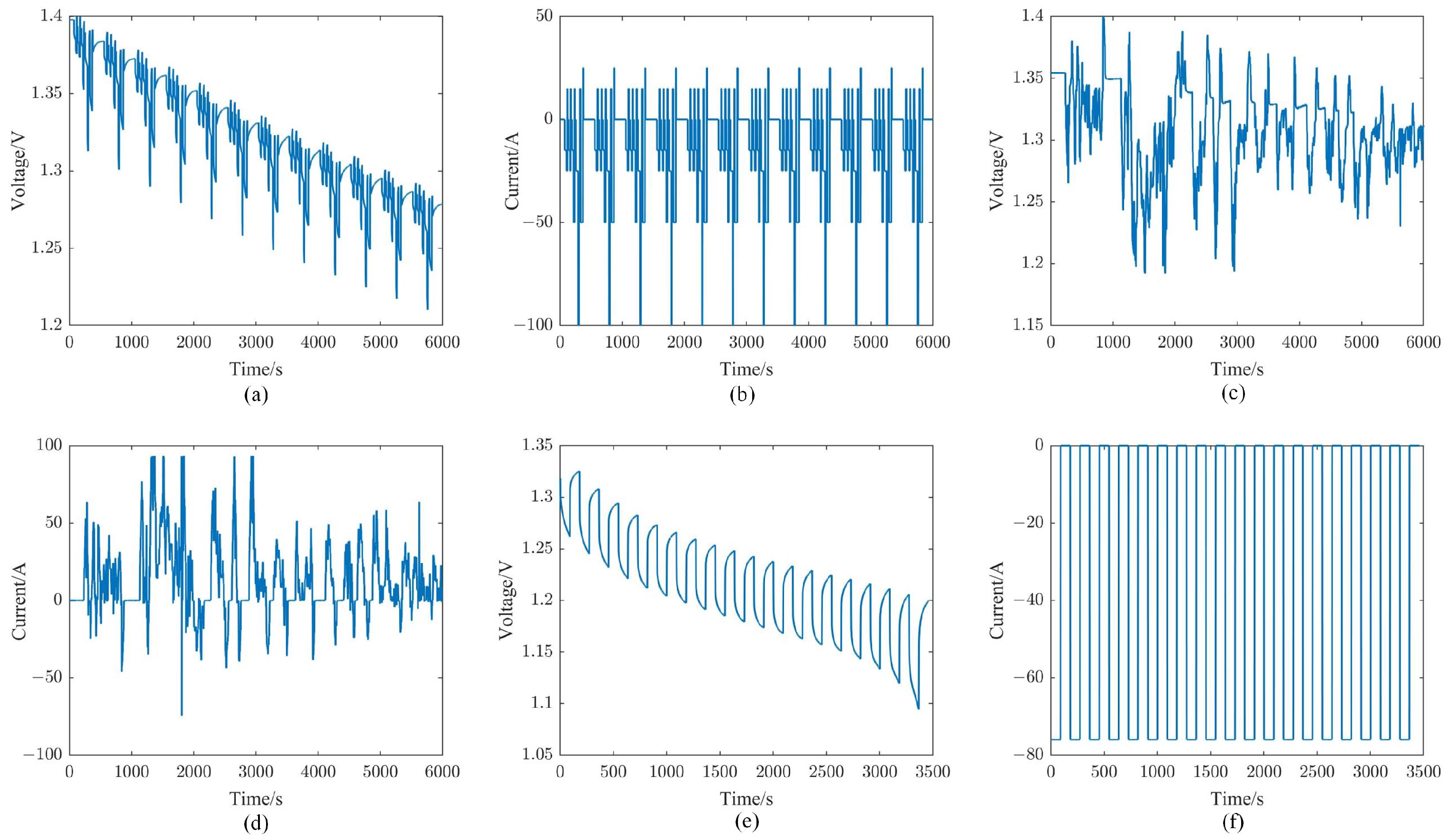
| DST | Step 1: The battery is discharged to the cutoff voltage (1 V) at a constant current rate of 0.5 C and a set temperature of 20 °C. Step 2: Static battery for one hour. Step 3: The battery is charged to the cutoff voltage (1.52 V) at a rate of 1 C and then charged to the cutoff current (20 A) at a constant voltage. Step 4: The charge-discharge cycle is set to 6 min and the charge-discharge experiment is carried out according to the DST power meter. |
| FUDS | Step 1: The battery is discharged to the cutoff voltage (1 V) at a constant current rate of 0.5 C and a set temperature of 20 °C. Step 2: Static battery for one hour. Step 3: The battery is charged to the cutoff voltage (1.52 V) at a rate of 1 C and then charged to the cutoff current (20 A) at a constant voltage. Step 4: Discharge under FUDS conditions. |
| Cyclic Pulse | Step 1: The battery is discharged to the cutoff voltage (1 V) at a constant current rate of 0.5 C and set temperature. Step 2: Static battery for one hour. Step 3: The battery is charged to the cutoff voltage (1.52 V) at a rate of 1 C and then charged to the cutoff current (8.5 A) at a constant voltage. Step 4: The discharge cycle is set to 15 min and the pulse-discharge experiment is carried out. |
| Model | Parameter |
|---|---|
| SVR | Kernel function: radial basis; Penalty factor: 2.5 |
| XGBoost | Number of decision trees: 200; Learning rate: 0.05; Depth of a single tree: 6 |
| GRNN | Smoothing factor: 0.2; Number of neurons: 100 |
| APSO-GRNN | Initial particle position: random numbers ranging from 0.01 to 0.5; Initial velocity weight: 1; Learning factor: 2 |
| SVR | 4.58 | 0.0237 | 0.9597 |
| XGBoost | 3.59 | 0.0184 | 0.9656 |
| GRNN | 3.86 | 0.0189 | 0.9534 |
| APSO-GRNN | 1.70 | 0.0107 | 0.9789 |
| SVR | 6.86 | 0.0378 | 0.9421 |
| XGBoost | 5.09 | 0.0326 | 0.9561 |
| GRNN | 7.11 | 0.0418 | 0.9452 |
| APSO-GRNN | 2.56 | 0.0176 | 0.9746 |
Disclaimer/Publisher’s Note: The statements, opinions and data contained in all publications are solely those of the individual author(s) and contributor(s) and not of MDPI and/or the editor(s). MDPI and/or the editor(s) disclaim responsibility for any injury to people or property resulting from any ideas, methods, instructions or products referred to in the content. |
© 2023 by the authors. Licensee MDPI, Basel, Switzerland. This article is an open access article distributed under the terms and conditions of the Creative Commons Attribution (CC BY) license (https://creativecommons.org/licenses/by/4.0/).
Share and Cite
Xu, H.; Yu, T.; Chen, C.; Wu, X. State-of-Charge Prediction Model for Ni-Cd Batteries Considering Temperature and Noise. Appl. Sci. 2023, 13, 6494. https://doi.org/10.3390/app13116494
Xu H, Yu T, Chen C, Wu X. State-of-Charge Prediction Model for Ni-Cd Batteries Considering Temperature and Noise. Applied Sciences. 2023; 13(11):6494. https://doi.org/10.3390/app13116494
Chicago/Turabian StyleXu, Haiming, Tianjian Yu, Chunyang Chen, and Xun Wu. 2023. "State-of-Charge Prediction Model for Ni-Cd Batteries Considering Temperature and Noise" Applied Sciences 13, no. 11: 6494. https://doi.org/10.3390/app13116494
APA StyleXu, H., Yu, T., Chen, C., & Wu, X. (2023). State-of-Charge Prediction Model for Ni-Cd Batteries Considering Temperature and Noise. Applied Sciences, 13(11), 6494. https://doi.org/10.3390/app13116494