Featured Application
This study provides a simplified approach to the flutter analysis of suspension bridges having two superposed decks. The George Washington Bridge engineering case is analyzed, in consideration of its historical relevance and age. The obtained results are compared with the predictions of simplified formulations available from other sources.
Abstract
We deal with the flutter analysis of the George Washington bridge, in both the single- and double-deck configurations of 1931 and 1962, respectively. The influence of the additional lower deck on the aerodynamic behavior is investigated. To overcome the lack of aerodynamic data, a simplified approach is followed based on Fung’s formulation, in which the flutter derivatives are expressed in terms of the real and imaginary parts of the Theodorsen function and of the steady-state aerodynamic coefficients of the deck cross-section. The latter are obtained by Computational Fluid Dynamics simulations conducted in ANSYS FLUENT, whereas the ANSYS Mechanical APDL finite element package is used to perform the flutter analyses. Two different methods for the application of the aeroelastic forces are employed for the double-deck configuration: (i) self-excited forces, based on flutter derivatives related to the whole cross-section, acting on the upper deck; and (ii) self-excited forces, based on flutter derivatives related to the single deck, simultaneously applied to the upper and lower decks. The obtained results are critically compared with theoretical predictions of simple formulas available from the literature; it is suggested that laboratory tests are needed since no experimental results seem to be available.
1. Introduction
Old bridges (conventionally, which are more than 50 years old), require special maintenance, accurate inspections, and a careful assessment of their safety conditions.
The conflict between economy and structural performance between the 19th and the 20th centuries led the design of long-span bridges to the development of very flexible and slender structures. The use of the elastic deflection theory allowed for very slender decks against static loads and shifted the design trend at that time from rigid trusses to slender edge girders. This evolution ended brutally with the Tacoma Narrows Bridge disaster due to the wind-induced flutter instability on 7 November 1940. From then on, any design of a flexible structure must assure the structure itself to be stable under the dynamic effects of wind loads. In fact, in addition to the already known static divergence due to the steady-state wind loads, flutter stability has become a governing criterion in the design of long-span suspension bridges. The objective of a (linear) flutter analysis is to predict the lowest critical flutter wind velocity and the corresponding flutter frequency.
A crucial point in flutter analysis is the definition of motion-dependent aerodynamic loads. The first analytical solutions were developed by Wagner [1] and Theodorsen [2] for thin airfoil. Theodorsen defined the self-excited forces as the superposition of circulatory and non-circulatory contributions, the former depending on the oscillation frequency and accounting for flow unsteady effects, and the latter independent of oscillation frequency and including inertial effects due to the moving fluid mass. Subsequently, Scanlan and Tomko exported some features of the Theodorsen’s results extending the formulation to bluff bodies, as bridge cross-sections. In this formulation, the wind loads induced by sectional harmonic motions are described by means of a linear format based on experimentally evaluated parameters, called “flutter derivatives”, that supply the lack of closed-form analytical formulations [3,4]. The relation between Wagner’s approach based on indicial functions, Theodorsen’s theory based on circulatory function and Scanlan’s flutter derivatives is well detailed in [5].
In the last decades, Scanlan’s formulation has been the most widely adopted, and the calculation of flutter derivatives has become an important step for any flutter analysis. Currently, the only method considered reliable for their calculation at the design stage is that of carrying out experimental tests on scale models in wind tunnels. Some notable examples are [6,7] for the Great Belt East Bridge and [8] for the Akashi Kaikyo Bridge; more recently [9] for the Jianghai Channel Bridge and [10] for the Hardanger Bridge.
To overcome costs and difficulties arising from wind tunnel testing, several efforts were made with the aim of developing some simplified methods for the calculation of flutter derivatives. Although these methods are not appropriate for the final design stage, they allow useful and versatile studies in early design phases. Some authors utilized the derivatives of the thin airfoil, as [11] for the Humber bridge. This simplification leads to relatively small errors when the bridges are characterized by streamlined cross-sections. Al-Assaf [12] adopted an alternative approach for open-truss stiffened suspension bridges: he estimated the aerodynamic derivatives based on the correlation between the thin airfoil derivatives and those of other bridges having a similar deck configuration. The method was applied to evaluate the flutter stability of the second Tacoma Narrows Bridge, with special focus on the effects of the side grates. Another simplified approach is given by the quasi-steady theory, in which the aerodynamic loads depend on the instantaneous relative velocity between the flow and the cross-section. In this framework the flow-induced forces are described by means of non-linear static relationships involving the wind angle of attack and the displacements of the structure. A linearization of this model allows a comparison with Scanlan’s semi-empirical approach and furnishes an expression of the flutter derivatives as functions of the steady-state aerodynamic coefficients of the cross-section [13]. These simplified expressions of the flutter derivatives are widespread for the streamlined deck cross-sections. Some works on the validity of this approach are [14,15,16] and some applications for the determination of the critical state can be found in [17,18,19]. In a recent work [20], a linear superposition of flat plate aerodynamics was adopted to estimate the flutter derivatives of streamlined multi-box deck sections. In that case, correction factors were introduced into the proposed analytical formulas to better fit the available experimental data. In the present paper, a simplified approach is used based on Fung’s formulation [21], in which the flutter derivatives are expressed in terms of the steady-state aerodynamic coefficients and of the real and imaginary parts of the Theodorsen function.
Two-dimensional Computational Fluid Dynamics (CFD) simulations were conducted in ANSYS FLUENT for the determination of the lift and moment coefficients, varying the wind attack angle. In recent years, the CFD approach gained importance with respect to the traditional experimental investigation. Some applications related to the bridge cross-sections are [22,23]. More recently, Brusiani et al. [24] pointed out that Reynolds-averaged Navier-Stokes (RANS) approach coupled with the k−ω SST turbulence model, identify the best compromise between accuracy and computational cost. The CFD framework also provides different approximate techniques for the direct calculation of flutter derivatives, some applications are: [25,26,27,28]. Nevertheless, the calculation of the steady-state aerodynamic coefficients requires simpler simulations compared to those required to compute the flutter derivatives, especially in terms of computational effort. In addition, the approximations introduced by a 2D geometrical representation, neglecting several appendages that could affect the aerodynamic behavior, do not justify the use of more refined methods.
Concerning flutter analyses, several methods can be found in literature [29,30], a method developed by Hua and Chen [31], which allows the analysis to be carried out with the FE package ANSYS Mechanical APDL, is adopted in this paper. The software, in fact, provides specific user-defined elements, through which it is possible to implement the motion-dependent aeroelastic forces as expressed in Scanlan’s formulation.
The George Washington suspension bridge was chosen as a case study, partly because of its historical significance. In fact, it was the first bridge whose main span exceeded one kilometer. The bridge was opened to traffic in 1931. It is characterized by a total length of 1450 m and a mid-span of 1067 m. Initially it was composed only of the upper level, whereas the lower deck was constructed from 1958 to 1962 because of the increasing traffic flow. Both configurations will be analyzed in the following: the original one with the single deck and the stiffened one with the two decks (Figure 1). The choice is also motivated by the peculiarity of the current bridge having two superposed decks. A similar configuration can be detected in the Verrazano-Narrows Bridge (USA), also having a great historical relevance, and in the Yangsigang Yangtze River bridge (China), which currently has the third longest span in the world after the Akashi Kaikyo bridge (Japan) and the recent 1915 Çanakkale bridge (Turkey), the current World record.
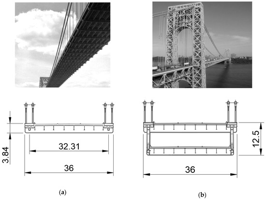
Figure 1.
George Washington bridge configurations (dimensions in m). (a) Single-deck, 1931; (b) Double-deck, 1962.
As a matter of fact, several investigations on the aerodynamic performances of trussed girders have been made, but only a few for double-deck bridges [32]. Due to the lack of aerodynamic data and studies on the subject, two simplified ways for the application of the aeroelastic forces are followed in the present study with the aim of obtaining approximate predictions. The first way considers the self-excited forces, based on the flutter derivatives related to the whole cross-section, acting on the upper deck. In the second case, the self-excited forces, based on the flutter derivatives related to the single deck, are simultaneously applied to the upper and lower decks. Both approaches produce plausible results, which can serve as a reference for future comparisons with alternative investigation methods. In principle, the proposed approach can be used for analyzing other double-deck bridges, and deserves further attention for proper validation.
2. Motion Related Wind Load
The equation describing the motion of the bridge in the smooth flow can be expressed as:
where, in a Finite Element framework, , , and represent the global mass, stiffness, and damping matrices, respectively; , , and are the nodal acceleration, velocity, and displacement vectors, respectively; and denotes the vector of nodal self-excited forces. The three degrees of freedom of the bridge deck cross-section, namely the vertical displacement , the torsional rotation , and the horizontal displacement , to which correspond the aeroelastic forces of lift , moment , and drag , are reported in Figure 2, where indicates the undisturbed mean wind velocity.
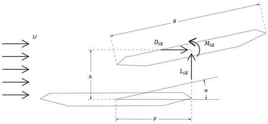
Figure 2.
Three-degrees-of-freedom section model.
According to Scanlan’s formulation [33], the self-excited aeroelastic forces per unit deck length can be expressed as a linear function of the displacement and velocity parameters of the deck as follows:
where is the air density, is the reduced circular frequency, and are the flutter derivatives. In most practical applications, ,, and () can be ignored.
As mentioned in the Introduction, the most reliable way to calculate flutter derivatives is based on experimental tests made in the wind tunnel. For the bridge chosen as a case study, no data regarding flutter derivatives were found in the literature, therefore a simplified approach was followed for their calculation. It was decided to utilize a formulation developed by Fung [21] for the thin airfoil because it allows one to input the slopes of the steady-state aerodynamic coefficients, and, unlike the quasi-steady approach, it provides a unique formulation for the determination of the derivatives . The expressions of the flutter derivatives are the following:
where and are the flutter derivatives for the thin airfoil as expressed by Fung (, and are respectively the real and the imaginary parts of the Theodorsen function, and are the derivatives of the lift and moment coefficients with respect to the wind angle of attack and is the distance between the shear center and the centroid of the airfoil, normalized with respect to the chord . For low values of reduced frequency, tends to one, tends to zero and the Fung formulation tends to the quasi-steady one.
These formulas were tested for two bridges of which both steady-state aerodynamic coefficients and flutter derivatives are available: the Great Belt East in Denmark, with a streamlined deck [6,34], and the Akashi Kaikyo in Japan, with a truss girder [35,36]. The derivatives of the aerodynamic coefficients, expressed in , are: and for the Great Belt Bridge; and and for the Akashi Kaikyo Bridge. The curves in Figure 3 and Figure 4 show a comparison between the flutter derivatives: obtained experimentally (solid crossed line), calculated by the Fung formulas (solid line), calculated by the quasi-steady formulation (dashed line) [26], and predicted by the Theodorsen theory for the thin airfoil (dash dotted line). From the comparisons in Figure 3 and Figure 4, it is possible to notice that the Fung formulation leads generally to a good alignment with the experimental curves: the average trend is always respected except for , that in some cases can be neglected [12]. A remarkable superposition is obtained for and of both bridges, and also for in the case of the Great Belt Bridge. Good predictions are also obtained for derivative.
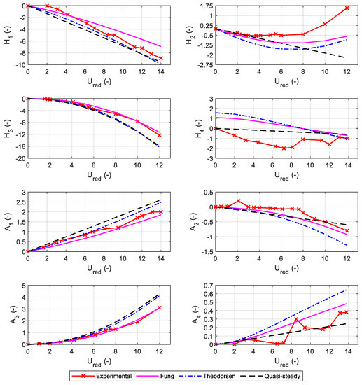
Figure 3.
Flutter derivatives of the Great Belt Bridge deck.
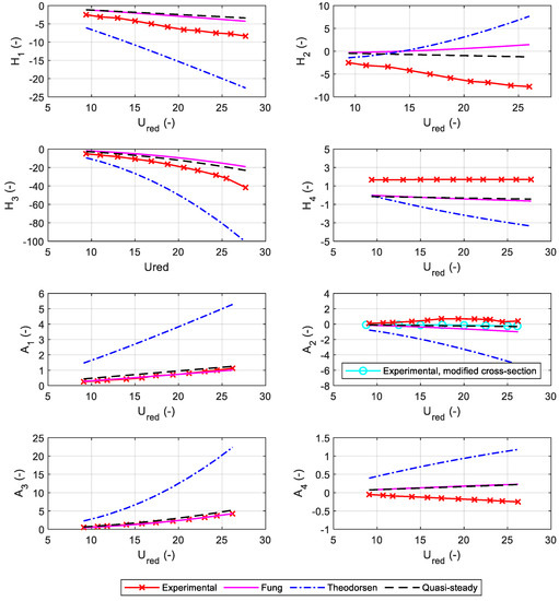
Figure 4.
Flutter derivatives of the Akashi Kaikyo Bridge deck.
As expected, for a truss-stiffened girder, Theodorsen formulation for thin airfoil becomes unable to reliably predict the aerodynamic behavior. Even though the quasi-steady formulation also shows a good agreement, the Fung formulation was chosen over the quasi-steady approach because this latter is better suited for low values of reduced frequency and high values of reduced wind velocities [16]. In fact, the bridge chosen as a case study is relatively stiff and characterized by high values of torsional and vertical eigenfrequencies, therefore flutter instability is expected to occur at a relatively low reduced velocity.
3. Full-Order Flutter Analysis Using ANSYS Mechanical APDL
The main lack of almost all the FE packages commonly used in civil engineering is the impossibility of including motion-dependent aeroelastic loads into the model and then of performing a complex eigenvalue analysis. Hua and Chen [31] proposed a method that allows one to perform a flutter analysis using the commercial finite element package ANSYS Mechanical APDL. The method is based on the definition of the aeroelastic loads by means of a particular user-defined element as shortly illustrated below. According to the method developed by Hua and Chen [31], the motion-dependent effect due to the wind load is considered for each deck element by the element aeroelastic stiffness and damping matrices modeled by the user defined MATRIX27 elements. Following Scanlan’s formulation, the self-excited forces are expressed as functions of the flutter derivatives, as recalled in Section 2.
It is possible to manipulate Equations (2a)–(2c) in order to obtain the equivalent nodal forces acting on the ends of the generic deck element, hence a lumped formulation can be used to derive the element aeroelastic stiffness and damping matrices [30]. Assembling the element matrices into global aeroelastic stiffness () and damping () matrices, the mathematical model of the system integrated with the effect of aeroelasticity is obtained [31]:
The global aeroelastic stiffness and damping matrices contain flutter derivatives, which depend on the reduced wind velocity (, oscillation frequency). Therefore, the system expressed by Equation (4) is parameterized by wind velocity and vibration frequency. By Equation (4), a complex eigenvalue analysis can be carried out to determine the critical wind velocity and vibration frequency. Being the conjugate pairs of complex eigenvalues , and the conjugate pairs of complex eigenvectors , the system will be dynamically unstable if the real part of any eigenvalue is positive. Hence, the condition for the onset of flutter instability is stated as follows: at a certain critical wind velocity , the system has only one eigenvalue with zero real part, and the imaginary part of the complex eigenvalue becomes the flutter frequency. It is necessary to provide the variation of both wind velocity and vibration frequency in the complex eigenvalue analysis, so that a mode-by-mode tracking method can be employed to iteratively search the flutter frequency and the flutter velocity [31].
The motion-dependent effect due to the wind is taken into account for each deck element by the element aeroelastic stiffness and damping matrices. These matrices should be properly compiled to implement the aeroelastic motion-dependent load by means of the flutter derivatives. User defined MATRIX27 element in ANSYS Mechanical APDL can only model either an aeroelastic stiffness matrix or an aeroelastic damping matrix instead of both of them simultaneously, so a pair of MATRIX27 elements must be attached to each node of a generic bridge deck element as illustrated in Figure 5. The MATRIX27 elements and represent respectively the aeroelastic stiffness and damping of the node , as the MATRIX27 elements and represent respectively the aeroelastic stiffness and damping of the node .
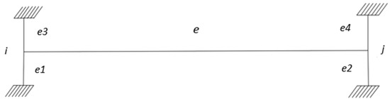
Figure 5.
Hybrid finite element model: “e”, structural element; “e1”, “e2”, “e3” and “e4”, MAYRIX27 aeroelastic element.
4. The George Washington Bridge
As mentioned in the Introduction, the two configurations of the George Washington bridge were chosen as case studies (Figure 1). The deck cross-sections of both configurations were modeled in ANSYS FLUENT, where the steady-state aerodynamic coefficients were calculated via CFD analyses. Finally, full bridge models were developed in ANSYS Mechanical APDL to perform structural and flutter analyses. Flutter derivatives characterizing the aeroelastic load of full bridge models were calculated by means of Equation (3), with and resulting from the CFD analyses.
4.1. Steady-State Aerodynamic Coefficients and Flutter Derivatives
Once the Fung formulation was validated, the steady-state aerodynamic coefficients of both the George Washington deck cross-sections were calculated in ANSYS FLUENT. For each section model and different wind attack angles, RANS simulations were performed modeling the turbulence by the method, following the indications in [24,37]. In order not to interrupt the logical flow of the speech, more information is given in Appendix A. The resulting steady-state aerodynamic coefficients of lift, , and moment, , are shown in Figure 6, where dashed lines represent the linear regressions. In the case of the double deck (Figure 6b), static coefficients deviate from linearity for higher angles of attack, so the linear regressions are restricted to the intervals and for lift and moment coefficients, respectively. The first derivatives of static coefficients at the origin, calculated as the slopes of linear regressions, are: , for the single-deck and , for the double-deck configurations.
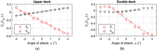
Figure 6.
Steady-state aerodynamic coefficients of lift and moment for the George Washington Bridge. (a) Upper deck; (b) Double-deck.
Flutter derivatives, calculated accordingly by means of Equations (3a)–(3h), are shown in Figure 7 and Figure 8. These were used to calculate the aerodynamic lift and moment actions to be applied to the bridge section.
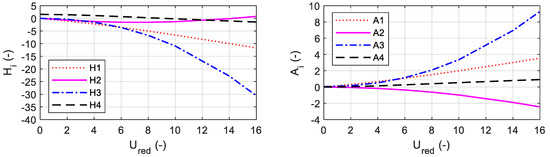
Figure 7.
Flutter derivatives of the George Washington Bridge’s upper deck according to Equations (3a)–(3h).
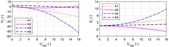
Figure 8.
Flutter derivatives of the George Washington bridge’s double deck according to Equations (3a)–(3h).
For the double-deck section, the lift and moment actions, based on static coefficients of the whole section, are applied to the top deck only, as sketched in Figure 9a. In addition, a second alternative method was adopted, which allows avoiding the use of data in Figure 6b and provides an additional model for comparison and validation of results. This latter method permits the same aeroelastic forces calculated for the single deck to be simultaneously applied to both upper and lower decks, as illustrated in Figure 9b. This procedure assumes that there is no aerodynamic interference between the two decks, whereas the mechanical interference is correctly modeled by the elements composing the truss. Furthermore, the pressure coefficients of the lower deck are assumed to be equal to those of the upper one and the aerodynamic influence of the secondary truss elements is also neglected. Despite the previous simplifications, the advantage of this procedure lies in the greater reliability of the results of CFD analysis for the single deck. Moreover, it can be conjectured that the simplified formulation previously introduced for the calculation of flutter derivatives (see Equations (3a)–(3h)), being based on the aerodynamics of the thin airfoil, is more suitable for the description of the behavior of a single deck rather than of a double deck.

Figure 9.
Sketch of the alternative methods adopted for the definition and application of aeroelastic loads to the double-deck cross-section. (a) Lift and moment actions, based on static coefficients of the whole section, applied to the top deck only; (b) Lift and moment actions, based on static coefficients of the single-deck section, applied to both upper and lower decks.
4.2. Finite Element Models
The ANSYS Mechanical APDL numerical models were realized with the geometrical properties found in literature [38,39,40]. The suspension cables were modeled as beam elements (BEAM188), with a circular cross-section of radius 0.573 m. An equivalent elastic modulus of 1.07 × 10¹¹ Pa was adopted in order to take in to account the influence of the side spans. The hangers were modeled using LINK180 elements, that transmit only tensile forces between the deck and the main cables. The floor system was modeled by means of equivalent beams having the properties listed in Table 1, wherein the V-shaped up-winds and the lower elements refer to the double-deck configuration. The following material properties were assigned to each element except the suspension cables: Young’s modulus = 2.1 × 10¹¹ Pa, Poisson’s ratio = 0.3 and mass density = 7860 kg/m3. Point mass elements (MASS21) were attached to the upper chords and to the equivalent longitudinal beams, both lower and upper, in order to model the inertial contribution of the sidewalk slabs, roadway slabs and other secondary elements. According to Dana et al. [39], a total dead load of 417 kN/m and 569 kN/m were obtained for the single-deck and the double-deck configurations, respectively. Lastly, the MATRIX27 elements were attached to each node of the equivalent longitudinal beams to model the aeroelastic forces in terms of aeroelastic stiffness and damping.

Table 1.
Geometrical properties of the truss girder of the double-deck George Washington Bridge.
According to the two different methods introduced in the previous section for the double-deck configuration, two different models were realized. In the first model, the pairs of MATRIX27 elements, compiled with the flutter derivatives in Figure 8, were attached only to the upper deck. Whereas, according to the second method, MATRIX27 elements, compiled with the flutter derivatives plotted in Figure 7, were attached to both upper and lower decks. The finite element models are shown in Figure 10.
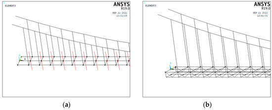
Figure 10.
ANSYS Mechanical APDL Finite element model. (a) Single-deck configuration (MATRIX27 elements are shown in red color); (b) Double-deck configuration (MATRIX27 elements are not shown).
5. Flutter Analyses
Before introducing the aeroelastic nodal forces by MATRIX27 elements, a modal analysis with no wind was performed: the results are summarized in Figure 11 and Figure 12, where the labels V, T, L stand for vertical, torsional and lateral, respectively; and the labels A and S stand for antisymmetric and symmetric, respectively. Since it is well known that flutter instability usually involves mainly the first modes at lower frequencies [31], only the first six modes were extracted for both configurations. The geometric nonlinearity of the structure was taken into account running the modal analysis in a preloaded configuration accounting for the gravity loads. Once eigenfrequencies and eigenmodes have been evaluated, the flutter analysis was performed by the method described in [31]. The aeroelastic loads were modeled as nodal forces affecting the stiffness and damping matrices of the element to which the nodes belong, so MATRIX27 elements were incorporated into the structural model to perform the damped eigenvalue analyses.
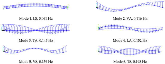
Figure 11.
Eigenfrequencies and eigenmodes of the single-deck configuration (1931).
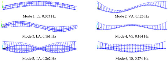
Figure 12.
Eigenfrequencies and eigenmodes of the double-deck configuration (1962).
Finally, the iterative procedure for the determination of flutter speed and frequency was carried out. The previous computational steps were followed for the eigenmodes collected in Figure 11 and Figure 12. The damped complex eigenvalue analyses were conducted for the model under different wind velocities. The step increment of wind velocity was set variable, from a maximum value of 10 m/s in the ranges far from the flutter instability to a minimum of 1 m/s close to the instability value. Accordingly, the resulting flutter wind velocity has the accuracy of one m/s. The variation of the complex eigenvalues vs. wind velocity is plotted in Figure 13, Figure 14 and Figure 15, where the labels within parentheses refer to the mode shapes under wind action: for instance, the label VT indicates a mode characterized by both vertical and torsional components, in which the vertical component is predominant. The real and imaginary parts of the eigenvalues represent the logarithm decay rates and damped vibration frequencies of these modes, respectively. As stated above, the flutter condition occurs when the real part of any eigenvalue becomes positive. The results obtained for the 1962 configuration refer to the two methods previously introduced and recalled hereafter:
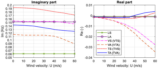
Figure 13.
Variation of complex eigenvalues vs. wind velocity for the single-deck configuration (labels within parentheses refer to mode shapes under wind action).
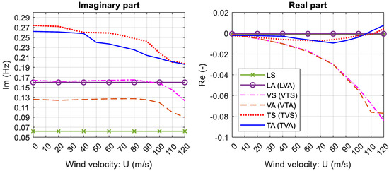
Figure 14.
Variation of complex eigenvalues vs. wind velocity for the double-deck configuration: first method (labels within parentheses refer to mode shapes under wind action).
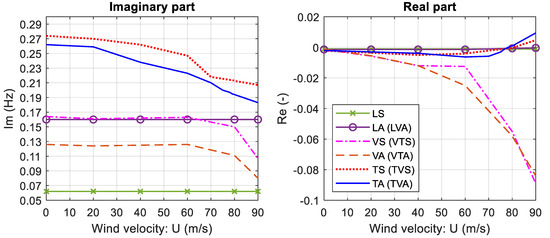
Figure 15.
Variation of complex eigenvalues vs. wind velocity for the double-deck configuration: second method (labels within parentheses refer to mode shapes under wind action).
The analyses furnished a critical flutter speed of 40 m/s (144 km/h) and a critical flutter frequency of 0.130 Hz for the single-deck configuration. As regards the double-deck configuration, flutter speeds of 107 m/s (385.2 km/h) and 79 m/s (284.4 km/h), and flutter frequencies of 0.203 Hz and 0.195 Hz, were provided by the first and the second method, respectively.
As already said, the variations of the imaginary part of the complex eigenvalues in Figure 13, Figure 14 and Figure 15 describe the change in the oscillation frequencies with the increasing wind speed, whereas the variations of the real part tell us about stability of each single vibration mode, and thus of the bridge deck. Accordingly, the first torsional-vertical anti-symmetric mode (TVA) is responsible for flutter instability in all the analyzed cases. For higher wind speeds, a second flutter mode is attained in the torsional-vertical symmetric mode (TVS); see Figure 13, Figure 14 and Figure 15. For the double-deck configuration, the first and the second flutter velocities are rather close, being close also the corresponding eigenfrequencies; see Figure 14 and Figure 15. In relation to that, we can say that interaction between modes having similar frequencies could be a triggering factor for instability, thus lowering the critical wind speed.
The two different methods adopted for the double-deck configuration furnish a difference of about 26% and 4% in the estimated critical wind speed and flutter frequency, respectively. Moreover, they provide similar frequency trends as wind speed increases and the same prediction of the flutter mode. Both introduce simplifications from the aerodynamic standpoint: in addition to the approximate evaluation of the flutter derivatives, the former method imposes the torsion rotation axis of the cross-section to coincide with the upper deck axis; the latter assumes that there is no aerodynamic interference between the two decks and neglects the influence of secondary truss-elements. Lastly, it should be noted that the use of flutter derivatives itself represents a strong simplification of the complex aerodynamic behavior of bluff bodies, as bridge decks.
Simplified Formulations and Comparisons
Given the absence of reference data for a direct validation, different simplified formulas available in the literature for predicting the flutter wind velocity were employed for a comparison. The results are collected in Table 2. The simplified formulas adopted are in Equations (5a)–(5f). The first one is based on the reduction of the divergence wind velocity ( and is the only one involving the aerodynamics of the deck by means of the derivative of the moment coefficient (). Equations (5b)–(5d) are empirical formulas fitted for thin airfoils, while Equations (5e) and (5f) contain a coefficient fitted for suspension bridge decks.
Table 2.
Flutter velocity according to different simplified formulations.
Frandsen [41]:
Selberg [42]:
Rocard [42]:
Matsumoto [43]:
Van der Put [44]
Fu and Wang [45]:
where , , , , . I is the polar mass moment of inertia per unit span length, m is the mass per unit span length, are the angular frequencies of the first vertical mode and the first torsional mode, are the respective frequencies and is an empirical coefficient representing the difference between the flat plate and a generic profile (equal to 0.7 for suspension bridges [44]). Other simplified formulations based on flutter derivatives can be found in [46].
Results provided by the different formulations for the single-deck configuration are similar to the ones obtained in the present work within the range . Larger variations are found for the double-deck configuration. In particular, formulas fitted for the thin airfoil provide a considerable overestimation of the critical speed with respect to the formulas fitted for the suspension bridges. The flutter limit provided by the first method is close to the prediction obtained by Equations (5b)–(5d), whereas the flutter velocity provided by the second method is closer to the predictions of Equations (5e) and (5f), and is the most conservative prediction.
Hence, although for a single-deck configuration having the aerodynamic coefficients similar to those of the airfoil it is possible to obtain reasonable results using simplified formulations, for a double-deck configuration it is necessary to perform more detailed analyses.
6. Discussion
The flutter stability of the George Washington bridge was investigated for the two different configurations, i.e., the original single-deck and the current double-deck. Due to the lack of literature data on the aerodynamic parameters for the bridge under consideration, two simplifications were introduced for the description of the motion-related wind loads: one for the calculation of flutter derivatives and the other for the application of aerodynamic loads on the two decks of the current configuration.
The method adopted for the calculation of flutter derivatives allows them to be obtained by analytical formulations based on the steady-state aerodynamic coefficients. The latter parameters were calculated by CFD simulations using the finite element software ANSYS FLUENT. The application of the method provided good results on the bridges chosen for validation, namely the Great Belt and the Akashi Kaykio. The main advantage lies in the relative simplicity of the calculation of the steady-state aerodynamic coefficients, on which the formulation is based. In fact, the computational cost required is much lower than that which characterizes the CFD analyses necessary for a direct numerical calculation of flutter derivatives. Of course, this approach furnishes approximate predictions. To further validate the method, comparisons should be extended to several bridge decks for which both steady-state aerodynamic coefficients and flutter derivatives are available. Once the flutter derivatives were defined, the flutter analysis was performed by a finite element ANSYS Mechanical APDL model endowed with MATRIX27 elements [31].
With regards to the double-deck configuration, two alternative methods were adopted for the definition and application of aeroelastic loads: a first one where lift and moment actions, based on static coefficients of the whole section, are applied to the top deck only; and a second one where lift and moment actions, based on static coefficients of the single-deck section, are applied to both upper and lower decks. Both methods introduce simplifications from the aerodynamic viewpoint. The former provides predictions similar to those of the simplified formulas calibrated for the airfoil. The latter is more aligned with the results provided by simplified formulations accounting for the difference between airfoil and deck cross-sections. With respect to the modal frequencies, the two methods provide similar trends for increasing wind speed, a 4% difference in the critical frequency estimation, and the same prediction of the flutter mode. According to the results of this study, the presence of the lower deck has raised the flutter wind velocity by more than 200%.
Although a definitive validation of the numerical results was not possible, due to the lack of experimental data, the authors believe that the results obtained here can be used for future comparisons with others obtained by different methods. In addition, the proposed approach provides an approximate way for estimating the flutter velocity of double-deck long-span bridges in the absence of more detailed analyses.
7. Concluding Remarks
Two simplified methods were adopted to achieve a preliminary flutter stability assessment of the double-deck George Washington Bridge. Both methods provided a realistic outcome, the second one seeming the most reliable and being the most conservative. The predicted critical flutter wind velocity is about 79 m/s (284 km/h). According to [47], for the bridge site, the wind speed corresponding to approximately a 1.6% probability of exceedance in 50 years is 129 mph (about 57.7 m/s). Given the lack of experimental data, it is suggested that wind tunnel tests are needed to obtain the flutter derivatives of the bridge deck.
Author Contributions
Conceptualization, A.C., G.P. and L.P.; data curation, G.P. and S.R.; formal analysis, S.R.; investigation, S.R.; methodology, G.P., L.P. and S.R.; resources: A.C., G.P. and L.P.; supervision, A.C.; validation, S.R.; visualization, S.R.; writing—original draft preparation, G.P. and S.R.; writing—review and editing, A.C. and L.P. All authors have read and agreed to the published version of the manuscript.
Funding
This research received no external funding.
Institutional Review Board Statement
Not applicable.
Informed Consent Statement
Not applicable.
Data Availability Statement
Some or all data, models or code that support the findings of this study are available from the corresponding author upon reasonable request.
Conflicts of Interest
The authors declare no conflict of interest.
Appendix A. RANS Simulations
The finite element package ANSYS FLUENT was chosen both for meshing and simulating the fluid flow around the rigid body, with the aim of integrating the pressure distribution and finally obtain the steady-state aerodynamic coefficients. For each deck cross-section model, a 2D RANS simulation was performed. The turbulence model, developed by [48], was adopted. This method consists in a sort of combination of the two simpler, widely used and models, whose weighting is controlled by the wall distance. Both are two-equation models, whose differences can be summarized as follows: the model does not allow for a direct integration of the field equations through the boundary layer because the parameter tends to zero close to the wall. Conversely, the model allows for directly integrating through the boundary layer, thus permitting to improve the goodness of the wall boundary layer unsteady-state solution, as demonstrated in [49]. As a drawback, the model has proved to be highly sensitive to inlet turbulence boundary conditions: this can sensibly affect the solution even in large computational domains [48]. To overcome this drawback, the model can conveniently be used. It preserves the main advantages of the classical model, but it has proved to be less sensitive to the inlet conditions.
After several tests regarding the turbulence model, the mesh sizing, the extension of the computational domain, and the boundary conditions, the following settings were adopted. Reference was made to [24,37] as a guide. For what concerns the computational domain, the outer rectangle in Figure A1 delimits the fluid region, the left and right sides representing the velocity inlet and the pressure outlet, respectively. The dimensions of the computational domain were set following the indication in [24]: around 12B (360 m) in the along-wind direction and 5.5B (180 m) in the transverse one. The cross-section centroid is located at a horizontal distance of 120 m from the velocity inlet. The domain is subdivided into different regions as shown in Figure A1. The circle and the inner rectangle were created as auxiliary geometric entities so to allow for a differentiated meshing of the region closer to the obstacle and of the wind wake. The circle and the inner rectangle have radius and height equal to 35 m for the single deck model and 40 m for the double-deck. Being the dimensions of the two models rather similar, the same mesh size was set for both the single- and the double-deck versions. As for the mesh, in the inner regions, the mesh dimension ranges from an edge size of 1 cm (order B × 10−3) to a maximum size of 25 cm (order B × 10−2), with a growth ratio equal to 1.1 [24]. In the fluid region between the outer boundary and the inner parts, a maximum size of 3 m (order B × 10−1) and a growth ratio of 1.2 were set. A quadrilateral mesh was chosen for each model to favor convergence and, thus, reduce the computational time. Figure A2 shows an example of meshed model of the double-deck George Washington Bridge, with different zoom levels.

Figure A1.
Computational domain for RANS simulation in ANSYS FLUENT (double-deck George Washington Bridge).

Figure A2.
Mesh for RANS simulation in ANSYS FLUENT (double-deck George Washington Bridge). (a) whole domain; (b) transition between sub-domains; (c) mesh around the deck; (d) detail around appendages.
Regarding the boundary conditions, the inlet was given a velocity of 30 m/s, a turbulent intensity of 0.5%, according to standard wind tunnel conditions for laminar flow, and a turbulent viscosity ratio equal to 2. The outlet was given a null pressure and the same turbulent intensity and viscosity as the inlet. The bridge deck edges were selected for the integration of the pressure distribution. The model parameters as the wind velocity, the chord length, and the air density were set so that dimensionless pressure coefficients were directly given by the program. Moment coefficients are referred to the upper deck centroid. To investigate different angles of attacks, several analyses were performed by rotating the bridge cross-section while keeping the boundary conditions and the computational domain unaltered. Results are summarized in Table A1. As an example, Figure A3 and Figure A4 show the distribution of velocity magnitude and pressure in the case of horizontal flow, with m/s, for the single-deck and the double-deck configurations of the George Washington Bridge, respectively. The simulations were run in a machine having the following main features: Intel® Core™ i9-12900K (30 MB cache memory, 8 P-core + 8 E-core, from 3.2 GHz to 5.2 GHz, 125 W); RAM 32 GB DDR5 memory, up to 4400 MHz; video card Nvidia RTX A4000, 16 GB, 4 DP; 64 bit operating system. The computational time required for meshing of each model was approximatively 40 min, while the computational time for RANS simulation was comprised between 5 and 10 min.
Table A1.
Resulting steady aerodynamic coefficients for different wind angles of attack.
Table A1.
Resulting steady aerodynamic coefficients for different wind angles of attack.
| Angle of Attack (°) | Single-Deck | Double-Deck | ||
|---|---|---|---|---|
| −3 | 0.123 | −0.09 | 0.107 | −0.035 |
| −2.5 | 0.030 | −0.075 | 0.128 | −0.038 |
| −2 | −0.028 | −0.058 | 0.112 | −0.045 |
| −1.5 | −0.042 | −0.041 | 0.064 | −0.050 |
| −1 | −0.159 | −0.021 | −0.043 | −0.047 |
| −0.5 | −0.163 | −0.007 | −0.120 | −0.038 |
| 0 | −0.252 | 0.013 | −0.287 | −0.023 |
| 0.5 | −0.274 | 0.026 | −0.357 | −0.004 |
| 1 | −0.334 | 0.047 | −0.516 | 0.018 |
| 1.5 | −0.427 | 0.061 | −0.529 | 0.035 |
| 2 | −0.441 | 0.075 | −0.730 | 0.074 |
| 2.5 | −0.522 | 0.097 | −0.712 | 0.074 |
| 3 | −0.538 | 0.103 | −0.762 | 0.090 |

Figure A3.
RANS simulation contours for single-deck George Washington Bridge section, zero attack angle, and m/s. (a) Velocity; (b) Pressure.

Figure A4.
RANS simulation contours for double-deck George Washington Bridge section, zero attack angle, and m/s. (a) Velocity; (b) Pressure.
References
- Wagner, H. Über Die Entstehung Des Dynamischen Auftriebes von Tragflügeln. ZAMM-Z. Angew. Math. Mech. 1925, 5, 17–35. [Google Scholar] [CrossRef]
- Theodorsen, T. General Theory of Aerodynamic Instability and the Mechanism of Flutter; NASA: Washington, DC, USA, 1935.
- Scanlan, R.H. The Action of Flexible Bridges under Wind, I: Flutter Theory. J. Sound Vib. 1978, 60, 187–199. [Google Scholar] [CrossRef]
- Scanlan, R.H.; Tomko, J.J. Airfoil and Bridge Deck Flutter Derivatives. J. Eng. Mech. Div. 1971, 97, 1717–1737. [Google Scholar] [CrossRef]
- de Miranda, S.; Patruno, L.; Ubertini, F.; Vairo, G. Indicial Functions and Flutter Derivatives: A Generalized Approach to the Motion-Related Wind Loads. J. Fluids Struct. 2013, 42, 466–487. [Google Scholar] [CrossRef]
- Larsen, A. Aerodynamic Aspects of the Final Design of the 1624 m Suspension Bridge across the Great Belt. J. Wind. Eng. Ind. Aerodyn. 1993, 48, 261–285. [Google Scholar] [CrossRef]
- Larsen, A. Aerodynamics of Large Bridges; Routledge: Oxfordshire, UK, 2017; ISBN 9781315136950. [Google Scholar]
- Miyata, T.; Yamaguchi, K. Aerodynamics of Wind Effects on the Akashi Kaikyo Bridge. J. Wind Eng. Ind. Aerodyn. 1993, 48, 287–315. [Google Scholar] [CrossRef]
- Chen, Z.-S.; Zhang, C.; Wang, X.; Ma, C.-M. Wind Tunnel Measurements for Flutter of a Long-Afterbody Bridge Deck. Sensors 2017, 17, 335. [Google Scholar] [CrossRef]
- Siedziako, B.; Øiseth, O.; Rønnquist, A. An Enhanced Forced Vibration Rig for Wind Tunnel Testing of Bridge Deck Section Models in Arbitrary Motion. J. Wind Eng. Ind. Aerodyn. 2017, 164, 152–163. [Google Scholar] [CrossRef]
- Brancaleoni, F.; Brotton, D.M. Analysis and Prevention of Suspension Bridge Flutter in Construction. Earthq. Eng. Struct. Dyn. 1981, 9, 489–500. [Google Scholar] [CrossRef]
- Al-Assaf, A. Flutter Analysis of Open-Truss Stiffened Suspension Bridges Using Synthesized Aerodynamic Derivatives. Ph.D. Thesis, Washington State University, Whitman, WA, USA, 2006. [Google Scholar]
- Caracoglia, L.; Jones, N.P. Time Domain vs. Frequency Domain Characterization of Aeroelastic Forces for Bridge Deck Sections. J. Wind Eng. Ind. Aerodyn. 2003, 91, 371–402. [Google Scholar] [CrossRef]
- Diana, G.; Bruni, S.; Cigada, A.; Collina, A. Turbulence Effect on Flutter Velocity in Long Span Suspended Bridges. J. Wind Eng. Ind. Aerodyn. 1993, 48, 329–342. [Google Scholar] [CrossRef]
- Larose, G.L.; Livesey, F.M. Performance of Streamlined Bridge Decks in Relation to the Aerodynamics of a Flat Plate. J. Wind Eng. Ind. Aerodyn. 1997, 69–71, 851–860. [Google Scholar] [CrossRef]
- Wu, T.; Kareem, A. Bridge Aerodynamics and Aeroelasticity: A Comparison of Modeling Schemes. J. Fluids Struct. 2013, 43, 347–370. [Google Scholar] [CrossRef]
- Borri, C.; Costa, C. Quasi-Steady Analysis of a Two-Dimensional Bridge Deck Element. Comput. Struct. 2004, 82, 993–1006. [Google Scholar] [CrossRef]
- Salvatori, L.; Spinelli, P. A Discrete 3D Model for Bridge Aerodynamics and Aeroelasticity: Nonlinearities and Linearizations. Meccanica 2007, 42, 31–46. [Google Scholar] [CrossRef]
- Øiseth, O.; Rönnquist, A.; Sigbjörnsson, R. Simplified Prediction of Wind-Induced Response and Stability Limit of Slender Long-Span Suspension Bridges, Based on Modified Quasi-Steady Theory: A Case Study. J. Wind Eng. Ind. Aerodyn. 2010, 98, 730–741. [Google Scholar] [CrossRef]
- Andersen, M.S.; Eriksen, M.B.; Larsen, S.V.; Brandt, A. The Influence of Gap- and Chord-Widths for Multi-Box Girders: Superposition of Flat Plate Flutter Derivatives and Section Model Tests. J. Fluids Struct. 2022, 109, 103489. [Google Scholar] [CrossRef]
- Fung, Y.-C. An Introduction to the Theory of Aeroelasticity; Dover Publications: Mineola, NY, USA, 2008. [Google Scholar]
- Vairo, G. A Numerical Model for Wind Loads Simulation on Long-Span Bridges. Simul. Model. Pract. Theory 2003, 11, 315–351. [Google Scholar] [CrossRef]
- Huang, L.; Liao, H.; Wang, B.; Li, Y. Numerical Simulation for Aerodynamic Derivatives of Bridge Deck. Simul. Model. Pract. Theory 2009, 17, 719–729. [Google Scholar] [CrossRef]
- Brusiani, F.; de Miranda, S.; Patruno, L.; Ubertini, F.; Vaona, P. On the Evaluation of Bridge Deck Flutter Derivatives Using RANS Turbulence Models. J. Wind Eng. Ind. Aerodyn. 2013, 119, 39–47. [Google Scholar] [CrossRef]
- Keerthana, M.; Harikrishna, P. Numerical Investigations on the Effect of Mean Incident Wind on Flutter Onset of Bridge Deck Sections. Struct. Eng. Mech. 2022, 82, 517–542. [Google Scholar]
- Montoya, M.C.; Nieto, F.; Hernández, S.; Kusano, I.; Álvarez, A.J.; Jurado, J.Á. CFD-Based Aeroelastic Characterization of Streamlined Bridge Deck Cross-Sections Subject to Shape Modifications Using Surrogate Models. J. Wind Eng. Ind. Aerodyn. 2018, 177, 405–428. [Google Scholar] [CrossRef]
- Li, J.; Quan, Z.; Zhang, Y.; Cao, L.; Li, C. Computational Fluid Dynamics Based Kriging Prediction on Flutter Derivatives of Flat Steel Box Girders. Symmetry 2022, 14, 1304. [Google Scholar] [CrossRef]
- Zhuo, L.; Liao, H.; Zhou, Q.; Li, M. Identification of Aerodynamic Derivatives of a Box-Girder Bridge Deck with Twin Active Flaps Using CFD Simulations. J. Bridge Eng. 2022, 27, 04022002. [Google Scholar] [CrossRef]
- Ding, Q.; Chen, A.; Xiang, H. A State Space Method for Coupled Flutter Analysis of Long-Span Bridges. Struct. Eng. Mech. 2002, 14, 491–504. [Google Scholar] [CrossRef]
- Namini, A.H. Analytical Modeling of Flutter Derivatives as Finite Elements. Comput. Struct. 1991, 41, 1055–1064. [Google Scholar] [CrossRef]
- Hua, X.G.; Chen, Z.Q. Full-Order and Multimode Flutter Analysis Using ANSYS. Finite Elem. Anal. Des. 2008, 44, 537–551. [Google Scholar] [CrossRef]
- Li, Y.; Tang, H.; Wu, B.; Zhang, J. Flutter Performance Optimization of Steel Truss Girder with Double-Decks by Wind Tunnel Tests. Adv. Struct. Eng. 2018, 21, 906–917. [Google Scholar] [CrossRef]
- Scanlan, R.H. Motion-Related Body-Force Functions in Two-Dimensional Low-Speed Flow. J. Fluids Struct. 2000, 14, 49–63. [Google Scholar] [CrossRef]
- Larsen, A. Advances in Aeroelastic Analyses of Suspension and Cable-Stayed Bridges. J. Wind Eng. Ind. Aerodyn. 1998, 74–76, 73–90. [Google Scholar] [CrossRef]
- Katsuchi, H.; Jones, N.P.; Scanlan, R.H. Multimode Coupled Flutter and Buffeting Analysis of the Akashi-Kaikyo Bridge. J. Struct. Eng. 1999, 125, 60–70. [Google Scholar] [CrossRef]
- Scanlan, R.H. Reexamination of Sectional Aerodynamic Force Functions for Bridges. J. Wind Eng. Ind. Aerodyn. 2001, 89, 1257–1266. [Google Scholar] [CrossRef]
- Tang, H.; Li, Y.; Wang, Y.; Tao, Q. Aerodynamic Optimization for Flutter Performance of Steel Truss Stiffening Girder at Large Angles of Attack. J. Wind Eng. Ind. Aerodyn. 2017, 168, 260–270. [Google Scholar] [CrossRef]
- Ammann, O.H. George Washington Bridge: General Conception and Development of Design. Trans. Am. Soc. Civ. Eng. 1933, 97, 1–65. [Google Scholar] [CrossRef]
- Dana, A.; Aksel, A.; Rapp, G.M. George Washington Bridge: Design of Superstructure. Trans. Am. Soc. Civ. Eng. 1933, 97, 97–163. [Google Scholar] [CrossRef]
- Dicker, D. Aeroelastic Stability of Unstiffened Suspension Bridges. J. Eng. Mech. Div. 1971, 97, 1677–1701. [Google Scholar] [CrossRef]
- Frandsen, A. Wind Stability of Suspension Bridges. Application of the Theory of Thin Airfoils. In Proceedings of the International Symposium on Suspension Bridges, Lisbon, Portugal, November 1966; pp. 609–627. Available online: https://trid.trb.org/view/105424 (accessed on 1 May 2023).
- Bartoli, G.; Mannini, C. A Simplified Approach to Bridge Deck Flutter. J. Wind Eng. Ind. Aerodyn. 2008, 96, 229–256. [Google Scholar] [CrossRef]
- Matsumoto, M.; Matsumiya, H.; Fujiwara, S.; Ito, Y. New Consideration on Flutter Properties Based on Step-by-Step Analysis. J. Wind Eng. Ind. Aerodyn. 2010, 98, 429–437. [Google Scholar] [CrossRef]
- Van der Put, T.A.C.M. Rigidity of Structures against Aerodynamic Forces; IABSE: Zurich, Switzerland, 1976. [Google Scholar]
- Fu, C.; Wang, S. Computational Analysis and Design of Bridge Structures; Taylor & Francis Group: Abingdon, UK; CRC Press: Boca Raton, FL, USA, 2017. [Google Scholar]
- Vu, T.-V.; Kim, Y.-M.; Han, T.-S.; Lee, H.-E. Simplified Formulations for Flutter Instability Analysis of Bridge Deck. Wind Struct. Int. J. 2011, 14, 359–381. [Google Scholar] [CrossRef]
- Minimum Design Loads and Associated Criteria for Buildings and Other Structures; American Society of Civil Engineers: Reston, VA, USA, 2021; ISBN 9780784415788.
- Menter, F.R.; Kuntz, M.; Langtry, R. Ten Years of Industrial Experience with the SST Turbulence Model. In Proceedings of the 4th International Symposium on Turbulence, Heat and Mass Transfer, Antalya, Turkey, 12–17 October 2003. [Google Scholar]
- Wilcox, D.C. Turbulence Modeling for Cfd, 3rd ed.; D C W Industries: La Canada, CA, USA, 1998. [Google Scholar]
Disclaimer/Publisher’s Note: The statements, opinions and data contained in all publications are solely those of the individual author(s) and contributor(s) and not of MDPI and/or the editor(s). MDPI and/or the editor(s) disclaim responsibility for any injury to people or property resulting from any ideas, methods, instructions or products referred to in the content. |
© 2023 by the authors. Licensee MDPI, Basel, Switzerland. This article is an open access article distributed under the terms and conditions of the Creative Commons Attribution (CC BY) license (https://creativecommons.org/licenses/by/4.0/).