Abstract
A promising class of devices for ocean wave energy conversion is called the oscillating water column in which the wave power is transferred to an airflow that rotates a turbine. A closed cycle power takeoff (CCPTO), in which air is forced through two valves and a turbine, has two main benefits for such a system: it allows a unidirectional turbine, and it smooths the large variations in pressure due to irregular (i.e., polychromatic) seas. This paper presents the design of a CCPTO for a shore-based installation, with particular attention paid to the turbine. The entire system is simulated with a reduced order model for a range of sea states to estimate the operating conditions of the turbine. It is found that the pressure drop range is modest but strongly dependent on the tide and sea chamber geometry. The geometry of the turbine is initially developed with a 1D preliminary design of the blades and then the turbine performance is analysed and the design is refined using Reynolds Averaged Navier–Stokes simulations. The design process is conducted based on the geometry and the sea climate of a real-life wave energy installation located in Mutriku (Spain). A turbine that displays efficient performance over a wide range of sea states is obtained. The overall performance of this turbine as part of the entire CCPTO system is assessed and leads to an energy output of ∼1500 kWh for one month in sea conditions at Mutriku wave power plant in Spain. It is concluded that the CCPTO deserves further development in any fixed oscillating wave column system.
1. Introduction
Ocean waves as a renewable energy source offer a relatively high energy density and limited impact on competing land uses (e.g., agriculture, tourism). Wave power has long been recognized as an attractive potential renewable energy source due to its high density and availability worldwide, with early attempts documented in the late 19th century [1]. The ready availability of petroleum suppressed interest in harvested energy sources such as wave power [2]. However, the oil shocks of the 1970s and the growing interest in low-carbon electricity production have resulted in a large variety of concepts at various stages of development. For example, in 2010, it was estimated that there were over 100 active wave energy projects [3], and it has been reported that there have been over 1000 different prototypes tested [4]. While Zhang et al. [5] have attempted to identify the “optimal” design concept, the indices used are open to debate. The difficulty in development is caused in part by the variability in the wave energy resource at a wide range of timescales due to individual waves (seconds), weather (days), seasonal variations (months) or even climatic events (years). Nonetheless, the resource has good predictability and is decorrelated with wind and solar power [6]. Furthermore, the potential resource is significant. For example, it has been estimated that the Northeastern Atlantic potential could be as much as 290 GW [7], while the global potential power of ocean waves impinging on coasts is estimated at 1 TW [3].
The first commercial wave energy converter (WEC) was designed by Masuda in Japan in 1965 and consisted of a floating oscillating water column (OWC) device [8]. In an OWC, the wave action drives the water in a chamber open to the sea, which in turn drives air through a turbine. While work continues on floating OWC devices for both the small scale (e.g., [9]) and large scale [10], there have been several examples of fixed OWCs, either shore-based (e.g., Pico, LIMPET) or bottom standing in shallow water near shore (e.g., OSPREY, Oceanlinx). The Pico plant was a 400 kW OWC with a Wells turbine commissioned in 1999 in the Azores, Portugal [11]. A similar 500kW device, called the LIMPET, was installed in Islay, Scotland [12]. The OSPREY in Scotland and the Oceanlinx in Australia were both large scale near shore, bottom standing OWC devices, but both were destroyed shortly after deployment. However, a comparable device was successfully deployed near Jeju Island, Korea [8], and interest in near shore installations of OWC devices is continuing (e.g., [13]). Wave energy conversion based on OWC devices whether floating or fixed offers several advantages: the mechanism is not submerged; the sea chamber can provide an effective gearing of the flow and perhaps the most useful is that the energy presented to the turbine (i.e., in the air) can be dramatically reduced by venting in highly energetic sea states [9]. The main disadvantage is that the flow of air across the turbine is bidirectional; i.e., the airflow reverses twice per wave cycle. This has been overcome to some extent with self-rectifying turbines (e.g., Wells, axial impulse or biradial turbines) [14], but these can have poor performance as the rotational speed of the turbine is nearly always mismatched to the instantaneous airflow velocity.
A closed cycle power takeoff (CCPTO) system consisting of two large air reservoirs connected by a unidirectional turbine has been proposed [15], and this arrangement was examined for a floating installation [16]. In those studies, the turbine performance was not considered directly.
In the CCPTO arrangement, shown conceptually in Figure 1, the power takeoff consists of three air chambers: the sea chamber, which is exposed to the OWC, the high pressure (HP) reservoir and the low pressure (LP) reservoir. The sea chamber is connected to the HP and LP reservoirs by non-return valves, while the HP and LP reservoirs are connected by the air turbine. Whether the sea level in the sea chamber of the OWC is rising or falling, the pressure in the HP reservoir is always above that in the LP reservoir, and thus the flow across the turbine is unidirectional. This is the principal benefit of this arrangement. An additional benefit is that, during excessive sea states, the turbine and generator set can easily be protected simply by venting the pressure chambers.
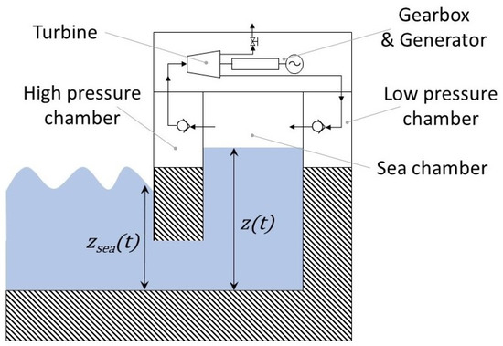
Figure 1.
Closed cycle power takeoff (CCPTO) for a shore-based installation. Pneumatic path including non-return valves and turbine through the sea; high-pressure chambers and low-pressure chambers indicated.
To understand the operation of the closed cycle PTO, consider the wave cycle as two half cycles: a compression process and an expansion process. During the compression process, the rising water surface in the sea chamber compresses air, raising the pressure, , in this chamber. For a short time, both valves are closed. This is not achieved by active control of the valves but by the temporal variation in the pressure in the three chambers. When the sea chamber pressure rises above the pressure in the HP reservoir, , the HP valve opens while the LP valve remains closed. For the remainder of the compression process, the OWC compresses all the system’s air through the HP reservoir, turbine and LP reservoir. Due to the pressure drop across the valves and turbine, the LP pressure, , is always lower than the HP pressure, . Hence, the LP valve remains closed during the OWC compression process.
During expansion, the opposite happens. The sea level drops in the sea chamber, reducing the pressure, until is below the HP pressure, , which causes the HP valve to shut off. As the pressure continues to drop, it will fall below the LP pressure, , causing the LP valve to open. From this point on, the expansion process is expanding the air in the HP and LP reservoirs into the sea chamber. The compressibility of the air means that the pneumatic spring effect is asymmetric around the equilibrium, with the compression cycle experiencing a harder spring than the expansion. Thus, the system is nonlinear, and it is necessary to model the CCPTO in the time domain. A reduced order model for the CCPTO is introduced in Section 2.1.
A key component of the system is the turbine: it is essential to ensure that an efficient turbine can be designed that is suitable for this application. To design the turbine, the specific conditions encountered in the CCPTO are needed. This includes characteristics such as the nominal pressure drop and mass flow rate, as well as their variation. To obtain realistic estimates of the turbine working conditions, the reduced order model of a CCPTO was applied to a notional shore-based installation that would be compatible with Mutriku breakwater. Mutriku is a fixed OWC structure installed into the breakwater at the entrance to the port of Mutriku, Spain. It is the world’s first multi-turbine wave energy facility and was first connected to the grid in 2011. The breakwater consists of 16 air chambers. In each chamber, an open cycle OWC system has been fitted with an 18.5 kW Wells fixed-pitch turbine, providing a total capacity to the plant of 296 kW, although in practice the actual achieved power is much lower (the capacity factor reported is 11% or an average power output of 28 kW [17]). Section 2.2 presents the results of the reduced order model for the breakwater at Mutriku. The turbine design process is then shown. It is divided into two parts: the preliminary 1D design in Section 2.3, followed by a CFD analysis and refinement in Section 2.4, yielding detailed performance characteristics. Finally, the resulting performances expected for the designed turbine in Mutriku’s breakwater are presented in Section 3.
2. Materials and Methods
2.1. System Modelling
The CCPTO is idealised as a closed pneumatic system, as shown in Figure 2. This is a similar approach to that previously adopted [15]. However, unlike the previous formulation in which the pressure in each chamber was the primary variable, in this formulation, the instantaneous mass in each chamber is determined directly from the sum of the mass flux through the valves and turbine. The mass flow rates are obtained from the volumetric flow rates, which depend on the instantaneous pressures in the system. In this way, mass is conserved, yielding a more robust model. This 1D model is crude as it excludes the full complexity of the internal flow and it is based on several assumptions:
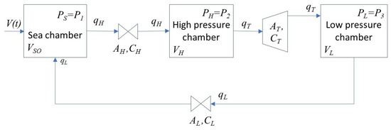
Figure 2.
Schematic of lumped parameter model of CCPTO.
- isentropic compression/expansion is assumed in all chambers;
- the sea surface acts as a rigid piston, so no sloshing is considered;
- air density at valves and turbines is assumed to be equal to the upstream value;
- a rudimentary turbine model is adopted. In effect, the turbine is represented as an orifice, with an area and a turbine coefficient, . This is justified by the detailed performance simulations of the turbine shown below.
The mass in each chamber can be decomposed into a mean and fluctuating component:
where for sea, high-pressure chambers and low-pressure chambers, respectively. Assuming the system starts at atmospheric conditions, the initial mass in each chamber is given by:
The principal solution variables are given by the first-order ordinary differential equations, which simply enforce mass conservation (Equations (3)–(5)). The mass flow rates through each component in Figure 2 are denoted as , where for flow through the turbine, low-pressure valve and high-pressure valve, respectively.
Sea Chamber mass flux:
High-Pressure Chamber mass flux:
Low-Pressure Chamber mass flux:
The density in each chamber is simply the mass divided by the volume:
The volumes, , of the high- and low-pressure chambers are fixed and the volume of the Sea Chamber is determined by the instantaneous water level:
and:
The entire system is driven by the perturbation from the equilibrium of the sea volume in the sea chamber caused by the incoming waves.
The flow rates in the system are obtained by treating both valves and the turbine as a simple flow restriction. It is given by:
where is a discharge coefficient and is proportional to the open area of the component. Note that, if the pressure difference is negative (i.e., ), the flow rate is 0. For the valves, the value of is 0.6, with a cross-sectional area of 1.5 m2. The corresponding values for the turbine are and . The density, , is assumed to be that of the upstream chamber, but this could be relaxed to be either an average of up- and downstream values or simply set to the reference value. Note that no account is taken of the shape of the ducting close to the valves or turbine. The effect of turbulence, flow separation and irrecoverable pressure drop are embedded in the assumed discharge and turbine coefficients. The instantaneous pressure is required in each chamber to calculate the flow rates. This is calculated based on an isentropic process. It is assumed that the entire system starts at pressure equilibrium conditions (i.e., the pressure and volume and density are atmospheric):
The volume of air in the sea chamber depends both on the incoming waves, i.e., the OWC motion, and on the back pressure imposed by the CCPTO. The coupling is achieved by solving the following differential equation:
where is the water column elevation, so that .
Equation (11) results from applying Newton’s second law of motion to the water column of fixed mass , height and cross-sectional area , subjected to the following list of forces.
Force exerted by the CCPTO back pressure:
Force exerted by the incoming waves:
Damping accounting for the water/walls friction losses:
The damping term R represents losses due to friction between the water column and the concrete walls of the chamber. is the water density, taken constant, is the water column mean velocity, is the contact surface area and is a friction coefficient approximated using a correlation with the Reynolds number of the flow. The value of was . The prime role of this damping term is to obtain a better understanding of the dynamic response of the system using a reasonable value for losses.
Finally, the hydrostatic forces to account for the weight of the water column and buoyancy forces are included. As these last two forces do not change, together they represent the equilibrium sea level and thus effectively define the sea chamber volume . They are included to allow the easy application of different tide heights.
2.2. Conditions at the Mutriku Breakwater
Measurements of the internal free surface heights in the sea chamber at Mutriku for 30 days in a typical month of April were made available by the operators through private communication. These measurements were taken with an open cycle PTO system in place. They are here assumed to be reasonably representative of open sea behaviour. The significant wave period and height were calculated using the spectral moment method [18]. Figure 3 presents the resulting wave climate, showing the probability of any given sea state to occur in Mutriku in April.
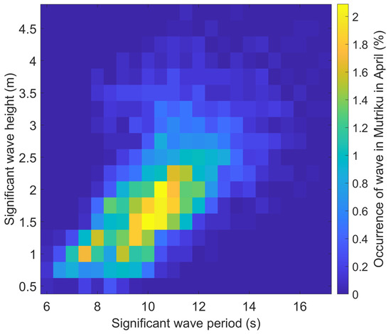
Figure 3.
Mutriku wave climate in a month of April.
A 1000 s sample was extracted from the measurements carried out in the sea chamber at Mutriku. The high-frequency components were filtered out to prevent unwanted noise. The sample was scaled to each of the wave heights and periods and then used as the input to the model. The size of the valves was chosen as m3, which is large enough to not restrict the flow, and the turbine size was selected as m3, at its maximum efficiency [19]. The resulting average power available at the turbine is shown in Figure 4. The highest power outputs occur for waves with the smallest periods and the largest heights. Similar results can be derived for low and high tides, showing that a higher tide results in a higher average power.
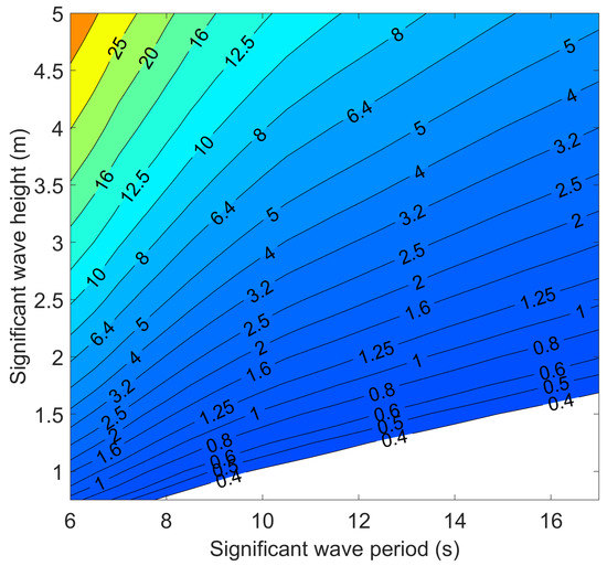
Figure 4.
Average power available at turbine for a polychromatic wave input of different standard heights and periods at mean tide (kW).
The choice of a nominal design point for the turbine is not straightforward as the operating conditions vary with the tide level and the sea state. A first idea is to design for the conditions that occur the most in the chosen site, which corresponds to for April in Mutriku, as visible in Figure 3. However, the sea state is nearly as frequent in Mutriku while being taller, more energetic waves. Figure 5 shows Mutriku’s climate weighted by the power available at the turbine. In effect, it is the result of the multiplication of Figure 3 and Figure 4. It should be noted that the order of magnitude agrees with the measured electric power actually generated by a turbine in Mutriku [17]. is then the most interesting design point. Table 1 presents the turbine operating conditions calculated using this model for both sea states of interest, and for three levels of tides: high, mean and low.
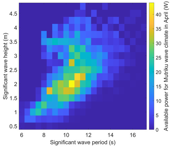
Figure 5.
Mutriku power-weighted wave climate in April.

Table 1.
Turbine operating conditions for different sea states and tide levels.
The results shown in Table 1 highlight the variability in the turbine operating conditions depending on the choice of design point. For those six cases, the mean pressure drop between the high-pressure and the low-pressure accumulators varies by between the less energetic case and the most energetic one, while the mean mass flow rate through the turbine varies by . Moreover, those are averages and the actual operating conditions for the turbine differ from wave to wave.
Figure 6a,b shows the distribution of, respectively, the mass flow rate and the pressure drop for the least and most energetic of the six cases considered in Table 1. Not only does the most energetic case lead to higher mean pressure drop and mass flow rate but it is also linked with more scattered distributions. The standard deviation of the mass flow rate distribution is 0.21 kg/s and 0.30 kg/s for the least and most energetic cases, respectively, while the standard deviation of the pressure drop is 876 Pa and 1860 Pa for the same two cases. The turbine design must ensure good efficiency over a wide range of operating conditions.
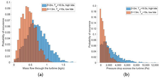
Figure 6.
Distribution of mass flow (kg/s) (a) and pressure drop (b) for the two extreme cases considered in Table 1.
2.3. Preliminary 1D Design of the Turbine
In this section, the process followed to obtain a suitable turbine design is presented. A complete description of such a work can be found in turbomachinery books (e.g., [20]). Out of the six cases presented in Table 1, two cases will be considered: the most energetic case (high tide, ) and the least energetic case (low tide, ).
The best-suited type of turbine for this high flow rate/small pressure drop application is an axial flow turbine, where the flow direction is perpendicular to the axis of rotation. It is the most common configuration for gas turbines and has the advantage of being efficient on a wider range of speeds than radial or mixed flow turbines. It is thus expected to be better able to extract power from a wide range of sea states. The turbine can be one stage only, which limits the costs and is more compact.
The specific speed is defined by
where is the rotational speed in rad/s, is the mass flow rate in kg/s, is the density in and is the isentropic enthalpy in J/kg. It represents the maximum available energy and can be calculated as follows
where is the specific heat capacity, and are, respectively, the inlet total temperature and pressure, is the outlet static pressure and is the heat capacity ratio. For an axial flow turbine, the optimal specific speed is about , as plotted by, for instance, [21]. This leads to an optimal rotational speed of and 1700 rpm for, respectively, the most energetic and the least energetic of the considered cases.
The turbine consists of a row of fixed blades called the stator, or the nozzle guide vanes, followed by a row of rotating blades called the rotor. In an impulse turbine, all the expansion occurs in the stator, while, in a reaction turbine, all the expansion occurs in the rotor. The degree of reaction is defined by
and is chosen in between those two extremes at , where the best performances are expected for this application.
Another important dimensionless design parameter is the velocity ratio
where is the axial flow velocity and U is the rotor blade speed at the mean radius. A small velocity ratio is usually linked to higher efficiencies, but it implies a larger turbine. Here, a velocity ratio of is taken, but that value could easily be modified depending on the physical constraints on the turbine size.
The last dimensionless design parameter to choose is the blade aspect ratio
where H is the height of the blades and b is their axial chord length. In this work, it was taken to be . This choice results from a compromise between keeping the turbine compact and ensuring that the tip clearance remains proportionally small.
Based on the turbine requirements obtained above for the breakwater at Mutriku, the turbine geometry can be determined. An important aspect of it are the rotor and stator blade angles. The blade angles are defined in Figure 7 and can be expressed in terms of the degree of reaction R and the velocity ratio (where is the axial velocity through the turbine), as follows
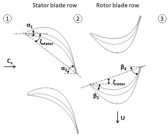
Figure 7.
Blade geometric parameters definition. Numbers indicating the location in the stage correspond to the subscripts on pressure, temperature and enthalpy.
In a single-stage turbine, the inlet angle . The stagger angles define the position of the blade chord relative to the axial direction. It was calculated assuming a circular arc camber line:
This leads to the angles presented in Table 2. As the angles depend on the choices of non-dimensional parameters only, they are the same for both cases considered.
Table 2.
Blade angles.
The blade height H and mean radius together define the turbine flow area . The area is determined by the air mass flow rate required to pass through the turbine. Indeed, seeing that the axial velocity is constant through the turbine, the mass flow rate is where is the air density.
Since the axial flow velocity is proportionally linked to the blade speed U through the design parameter , the problem reduces to the estimation of the blade speed, which is completed by considering the total-to-total efficiency [20]:
where is the work produced by the turbine and is the isentropic enthalpy drop across the turbine, which was already calculated in Equation (18) based on the pressures obtained by the lumped model of the complete system. Using the relations linking the blade angles and the design parameters for , the work output can be written as
Thus, Equation (27) can be used to estimate the blade speed U by assuming the nominal total-to-total efficiency. Choosing , the nominal blade speeds obtained for the higher and the lower energy cases are, respectively, and 28.9 m/s. The mean radius is then simply derived as .
The resulting blade dimensions are presented in Table 3. Note that the geometry does not differ much between the two cases; the relative difference between the two blade heights or the two blade mean radii is . Indeed, the different mass flow rates are accounted for by different nominal speeds rather than different geometries. The rest of this study will, therefore, focus on one turbine design only, whose geometric parameters are taken as the average between those two cases.
Table 3.
Turbine dimensions.
The last design aspect to be determined is the number of stator and rotor blades. If there are many blades, the friction losses will be large; conversely, if there are very few blades, the fluid will lack guidance. An optimum can be found between these two extremes. This is usually completed using Zweifel’s criterion. The Zweifel’s number is:
Here, s is the pitch, i.e., the space between blades, b is the blade chord, and are the inlet and outlet angles. For the rotor, these are changed to and . Zweifel’s criterion predicts that the optimum pitch/chord ratio is obtained for . However, this led in our case to higher mass flow rates than required. It was thus decided to increase the number of blades to 21 stator blades and 29 rotor blades, which corresponds to .
2.4. Detailed Estimation of Turbine Performance
The CFD simulations were conducted using the tools of the commercial software ANSYS version 2021 R2. First, the blades were designed separately on BladeGen. The profile was drawn using the angles and the chord length previously determined, and it was stacked up straightly to the desired height. The geometry has been meshed using Turbogrid. A grid independence study was conducted.
The solver used was CFX. The steady-state compressible 3D RANS equations of mass, momentum and energy were solved using a second order discretisation scheme. As the Reynolds number is about , the turbulence model needs to be able to handle laminar to turbulence transition. The model used was thus the SST (Shear Stress Transport) model gamma-theta. The fourth order Rhie–Chow pressure dissipation algorithm was selected. The problem was considered converged when the residuals were below . The simulation was run across 12 CPUs as a parallel task using the Metis partitioner.
Figure 8 summarises the numerical setup. Since all blades are identical, only one blade is simulated, and the lateral boundaries are periodic. The two domains, one for the stator blade and the other for the rotor blade, are interfaced by a mixing plane. This boundary is defined as the circumferential averaging of the flow upstream and downstream. Although nonphysical, this numerical procedure has been shown to achieve good agreement with experimental measurements [22,23]. The blades, the hub and the shroud are non-slip adiabatic walls.
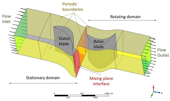
Figure 8.
Numerical domains and boundary conditions.
The total pressure and temperature are defined at the inlet, and the static pressure at the outlet. The only velocity defined is the rotational speed N of the rotating domain; hence, the mass flow rate is a result of the simulation. A range of values for the three parameters , and N were explored to be representative of the range of turbine conditions encountered in Mutriku’s breakwater.
2.5. Grid Convergence Analysis
To assess how dependent the results are on the mesh fineness used, the same problem was solved using six different grids consisting of a growing number of cells. The six meshes are presented in Table 4, with the time needed to perform each simulation. Eight different simulations were performed on each grid with a rotational speed and a pressure drop ranging from 600 to 3400 Pa in increments of 400 Pa.
Table 4.
Mesh characteristics.
As the mass flow rates obtained on the different meshes are quite close to each other, Figure 9 shows the relative difference in mass flow rate on each mesh with the one obtained on the very fine mesh. All of the results diverge by a few percentage points. The finer the mesh, the closer the resulting mass flow rate is to the very fine mesh result. The results on the medium mesh are 1% or less away from the results on the very fine mesh. They also need about 20 min per design point to compute, four times less than the very fine mesh simulations, which is deemed reasonable in practice.
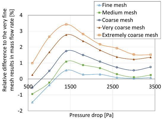
Figure 9.
Relative difference in mass flow rate at for different meshes compared to the very fine mesh.
Figure 10 shows the torque efficiency as a function of pressure drop obtained for the different meshes. The torque efficiency is defined as
where is the torque in Nm and is the rotational velocity in rad/s. Discrepancies can be observed in the results on different meshes. Close to the nominal design point, the simulations on a coarser mesh slightly underestimate the efficiency, while, at lower pressure drop, they overestimate it compared to the very fine mesh. The largest differences are observed for the lowest pressure drops where all results are quite scattered. For pressure drops over 1000 Pa, the medium mesh leads to results 1% or less away from the very fine mesh. It is thus the mesh refinement that will be used for every following simulation.
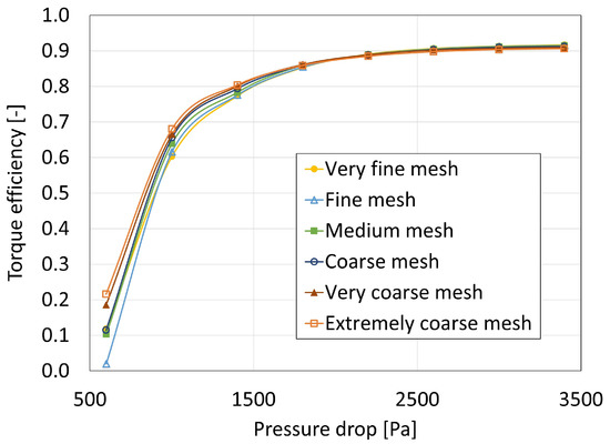
Figure 10.
Torque efficiency at for different meshes.
2.6. 1D Design Results
The simulation was carried out for 54 different design points, with rotational speeds ranging from 500 rpm to 3000 rpm and pressure drops ranging from 600 Pa to 3400 Pa for all rotational speeds, and up to 8200 Pa for . Following [14], the results are presented in their dimensionless form. In addition to the torque efficiency previously defined, the dimensionless pressure drop and the flow coefficient are as follows
It can be noted that the flow coefficient is proportional to the velocity ratio used in the preliminary design Section 2.3. Indeed, the mass flow rate is proportional to the axial velocity and the rotational speed is proportional to the blade speed.
Figure 11 shows the torque efficiency of the turbine for various flow coefficients. At the nominal design point, the efficiency reaches . However, the actual efficiencies are expected to be lower as some losses have been overlooked. In particular, the tip leakage losses are missing as the shroud is perfect here, with no gap between the shroud and the blades. The efficiency remains high after the peak, which supports the expectation for the turbine to be well suited to a range of sea states.
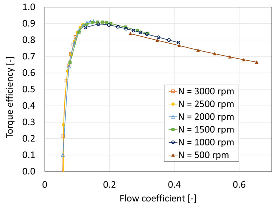
Figure 11.
Variation in efficiency with flow coefficient for different rotational speeds.
Figure 12 shows the dimensionless pressure drop variation with flow coefficient. The pressure drop curves follow a quadratic tendency. This supports the choice of modelling the turbine as a pure flow restriction in the lumped parameter model, where the mass flow follows Equation (9). The curves collapse with the non-dimensionalisation, which means that, even though is not truly constant when the rotation speed changes, its variation is limited. At lower rotation speeds, the turbine allows the passage of a larger mass flow than at higher rotation speeds for the same pressure drop. varies monotonously from m2 at N = 3000 rpm to m2 at N = 500 rpm, which is a difference. By comparison, the maximum efficiency obtained from the 1D Matlab model of the complete system for the Mutriku case was reached for . The turbine is thus on the safe side of the optimum peak, considering that the losses have been underestimated in the CFD study.
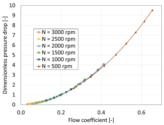
Figure 12.
Variation in pressure drop with flow coefficient for different rotational speeds.
2.7. Design Refinement
The preliminary design bases all calculations on a point at the mid height of the blade. This overlooks the variation in velocities across the blade in the spanwise direction. According to [24], if the hub–tip ratio is greater than 0.8, which means that the blade height is relatively small compared to the rotor radius, the two-dimensional flow assumption is reasonable. In this study, the hub–tip ratio was 0.73.
Two approaches have been taken to refine the design. First approach is leaning the blade, which consists of stacking the same blade shape developed in the preliminary design but with an angle in the radial direction. The aim is to counteract the radial pressure gradient created by the variation in centripetal force along the blade. The second approach is varying the blade angles radially, i.e., the free vortex design. Figure 13 presents a visualisation of these two approaches, which can be compared to the straight blade previously shown in Figure 8.
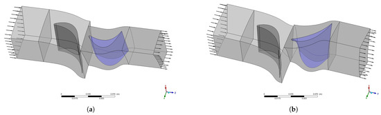
Figure 13.
Leaned rotor blade (a) and free vortex design blades (b).
The free vortex condition states that remains constant for all radii r, where is the swirl (or whirl) velocity. Combined with the conditions of constant axial velocity and constant specific work through the turbine, the free vortex condition ensures that the flow is in radial equilibrium. In practice, this means varying the blade angles so that
and
The resulting angles at the hub and the shroud are presented in Table 5. With varying angles, the degree of reaction will also vary, from at the hub to at the shroud.
Table 5.
Free vortex design blade angles.
Figure 14 shows the turbine’s efficiency for three blades: the straight blade obtained from the preliminary design, the leaned blade and the free vortex design blade. The leaned blade results collapse quite well with the straight blade ones. The free vortex blade improves the peak efficiency by 1 percentage point, from to . The efficiencies are also improved by the free vortex design at low flow coefficients, with a wider plateau of high efficiencies. However, they are slightly worsened at very high flow coefficients.
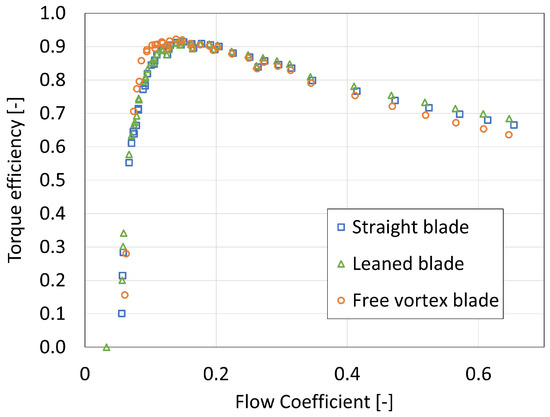
Figure 14.
Variation in efficiency with flow coefficient for different blade geometries.
Figure 15 shows a visualisation of the flow by plotting velocity streamlines around the straight blade and the free vortex design blade at N = 2000 rpm and Pa, which is the point of peak efficiency in Figure 14. There is a recirculation zone on the pressure side of the straight rotor blade, while the flow closely follows the shape of the free vortex blade. Moreover, the velocities on the suction side of the straight blade are higher compared to the free vortex blade. This explains the improvement in efficiency brought about by the free vortex design.
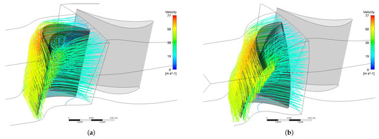
Figure 15.
Velocity streamline of the flow around the straight (a) and the free vortex design (b) rotor blade at nominal flow coefficient.
The straight blade is, however, expected to be easier to manufacture than the free vortex blade. In both cases, variations from the ideal design are expected during the manufacturing process. The variation in efficiencies remains at most a couple of percentage points when altering the 3D design of the blades. This shows that the turbine design is overall quite robust and can be expected to withstand manufacturing irregularities.
3. Results
In order to investigate the behaviour of the CCPTO and turbine in the real environment of the breakwater at Mutriku, the CFD study was extended to the larger pressure drops that infrequently occur in the case of larger waves. Sixty additional design points were explored, with pressure drops ranging from 3800 to 21,000 Pa and rotation speeds up to 5000 rpm. Figure 16 presents the resulting efficiencies for two cases: the straight blade from the preliminary design and the free vortex design blade. Increasing the rotational speed at high-pressure drop allows to maintain and even increase the turbine performances. As would be expected, the free vortex design consistently leads to better results than the straight blade, especially at peaks where the rotational speed is exactly optimised for the pressure drop. Although the improvement is modest, the free vortex design turbine will thus be used for the rest of the study.
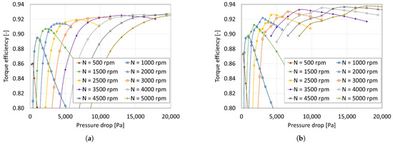
Figure 16.
Variation in efficiency with pressure drop for the straight blade (a) and the free vortex design blade (b).
The performances were computed in increments of 500 rpm in this study, but finer increments could be used to enhance the reliability of the estimation of overall system power predictions. Figure 17 shows the suitable rotational speed to adopt for the free vortex design turbine in each case at mean tide in Mutriku and the associated efficiency. Note that the actual efficiencies will be lower since various sources of losses have been neglected, particularly the tip leakage. Nevertheless, the speed-adjusting strategy is validated by these results.
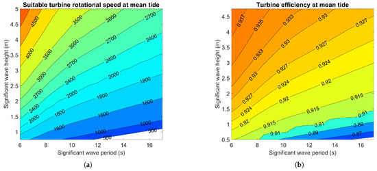
Figure 17.
Free vortex design turbine rotational speed (rpm) (a) and associated efficiency (b) for different sea states in Mutriku at mean tide.
Using these efficiencies, a further step can be taken from the power available at the turbine in Figure 4 to the power generated by the turbine, which is presented in Figure 18. A slight shift in the contour lines toward the upper left corner between these two figures can be observed. Finally, based on the corrected power output, the energy expected to be generated by this turbine for each sea state in April in Mutriku is calculated. It is shown in Figure 19. This estimation assumes that the tide is constant at mean level during the entire month of April. The sum of the matrix is 1544 kWh; it represents the total energy expected to be produced in that month. The outcome is a rough estimate, but it illustrates the expected benefits of the CCPTO arrangement for an oscillating water column installation.
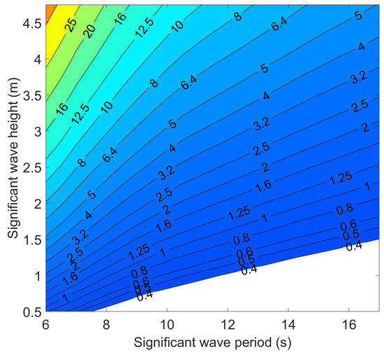
Figure 18.
Average power generated by the turbine at mean tide (kW).
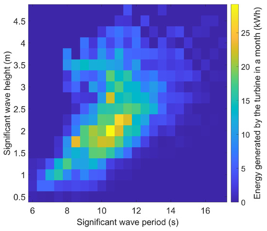
Figure 19.
Energy generated by the turbine in April in Mutriku (kWh).
4. Discussion
In this paper, the complete process of designing a turbine suitable for the closed cycle power takeoff of an oscillating water column device in a shore-based installation has been presented using the breakwater at Mutriku as a case study. Multiple tools were used, from a reduced order model of the entire system to an elementary 1D theory of axial flow turbine and 3D CFD simulations of the blades. The combination of different levels of study with consistent outputs strengthened the authors’ confidence in the suitability and performance of the designed turbine. In particular, the assumption of representing the turbine as an orifice in the reduced order system model agrees with the 3D CFD study, with a consistent turbine size metric.
The total energy captured over the month was 1544 kWh, yielding an average power of 2 kW. Most of this is obtained from sea conditions presenting less than 5 kW at the turbine (see Figure 4 and Figure 5). Thus, in principle, a suitably sized generator could be operated at a capacity factor of approximately since the CCPTO smooths the variability in the pressure at the turbine. It is worth noting that the sea chamber at Mutriku was designed for an open cycle, self-rectifying turbine. A smaller sea chamber volume would increase the maximum pressure achieved and thus increase the average power production but would not change the capacity factor significantly.
The process followed in this paper to design a turbine suitable for the breakwater at Mutriku is the basis for an optimisation strategy that could be applied to any fixed oscillating water column structure. It is a crucial step in the development of the closed cycle power takeoff in that it shows that the turbine is not a technological obstacle for this type of device. Future work will focus on the detailed design of the other system elements, such as the valves and the chambers, and, in the case of installations such as Mutriku, could consider the pressurization of the high-pressure chamber from multiple sea chambers.
Author Contributions
Conceptualization, C.M.; methodology, M.B. and L.G.; formal analysis, M.B. and L.G.; data curation, M.B. and L.G.; writing—original draft preparation, M.B.; writing—review and editing, C.M. and M.B.; project administration, C.M.; funding acquisition, C.M. All authors have read and agreed to the published version of the manuscript.
Funding
This research was funded by Sustainable Energy Authority of Ireland grant number SEAI/RDD/495.
Data Availability Statement
The data presented in this study are available on request from the corresponding author. The data are not publicly available due to some of them being proprietary.
Conflicts of Interest
The authors declare no conflict of interest.
Abbreviations
The following abbreviations and symbols are used in this manuscript:
| CCPTO | Closed Cycle Power Takeoff | |
| CFD | Computational Fluid Dynamics | |
| HP | High pressure | |
| LP | Low Pressure | |
| OWC | Oscillating Water Column | |
| PTO | Power Takeoff | |
| RANS | Reynolds Averaged Navier–Stokes | |
| SST | Shear Stress Transport | |
| WEC | Wave Energy Conversion | |
| A | Cross Sectional Area | m |
| b | Turbine chord | m |
| Friction coefficient between water and wall in Sea Chamber | - | |
| Loss coefficient in high-pressure valve | - | |
| Loss coefficient in low-pressure valve | - | |
| Loss coefficient in turbine for reduced order model | - | |
| Specific heat capacity for constant pressure | J/kg/K | |
| Axial airflow velocity in turbine | m/s | |
| F | Hydrodynamic force | N |
| h | Enthalpy | J/kg |
| H | Turbine blade height | m |
| Mean height of water column | m | |
| Total instantaneous air mass in chamber i () | kg | |
| Air mass fluctuation in chamber i () | kg | |
| Mass of water in water column | kg | |
| P | Pressure | Pa |
| Mass flow rate through CCPTO component | kg/s | |
| R | Degree of reaction | - |
| Mean radius | m | |
| S | Hydrostatic force per unit height | N/m |
| Air temperature at location k in turbine stage () | K | |
| Wave period | s | |
| U | Translational turbine speed at mean radius | m/s |
| Volume of chamber i () | m | |
| Water column mean velocity | m/s | |
| z | Sea level height | m |
| Significant wave height | m | |
| Rotational speed | rad/s | |
| Specific speed | - | |
| Ratio of heat capacities | - | |
| blade inlet angle | rad | |
| blade outlet angle | rad | |
| stagger angle of blade | rad | |
| Turbine efficiency | - | |
| Torque | Nm | |
| Pressure drop coefficient | - | |
| Flow coefficient | - | |
| Fluid density | kg/m |
References
- McCormick, M. Ocean Wave Energy Conversion; Wiley: Hoboken, NJ, USA, 1981. [Google Scholar]
- Falnes, J. A review of wave-energy extraction. Mar. Struct. 2007, 20, 185–201. [Google Scholar] [CrossRef]
- Falcão, A.F.d.O. Wave energy utilization: A review of the technologies. Renew. Sustain. Energy Rev. 2010, 14, 899–918. [Google Scholar] [CrossRef]
- Penalba, M.; Giorgi, G.; Ringwood, J.V. Mathematical modelling of wave energy converters: A review of nonlinear approaches. Renew. Sustain. Energy Rev. 2017, 78, 1188–1207. [Google Scholar] [CrossRef]
- Zhang, Y.; Zhao, Y.; Sun, W.; Li, J. Ocean wave energy converters: Technical principle, device realization, and performance evaluation. Renew. Sustain. Energy Rev. 2021, 141, 110764. [Google Scholar] [CrossRef]
- Fusco, F.; Nolan, G.; Ringwood, J.V. Variability reduction through optimal combination of wind/wave resources – An Irish case study. Energy 2010, 35, 314–325. [Google Scholar] [CrossRef]
- Clément, A.; McCullen, P.; Falcão, A.; Fiorentino, A.; Gardner, F.; Hammarlund, K.; Lemonis, G.; Lewis, T.; Nielsen, K.; Petroncini, S.; et al. Wave energy in Europe: Current status and perspectives. Renew. Sustain. Energy Rev. 2002, 6, 405–431. [Google Scholar] [CrossRef]
- Falcão, A.F.; Henriques, J.C. Oscillating-water-column wave energy converters and air turbines: A review. Renew. Energy 2016, 85, 1391–1424. [Google Scholar] [CrossRef]
- Henriques, J.; Portillo, J.; Gato, L.; Gomes, R.; Ferreira, D.; Falcão, A. Design of oscillating-water-column wave energy converters with an application to self-powered sensor buoys. Energy 2016, 112, 852–867. [Google Scholar] [CrossRef]
- Rosati, M.; Henriques, J.; Ringwood, J. Oscillating-water-column wave energy converters: A critical review of numerical modelling and control. Energy Convers. Manag. X 2022, 16, 100322. [Google Scholar] [CrossRef]
- Falcão, A.F. The shoreline OWC wave power plant at the Azores. In Proceedings of the Fourth European Wave Energy Conference, Aalborg, Denmark, 4–6 December 2000; p. B1. [Google Scholar]
- Heath, T.; Boake, C. The Design, Constructiona dn Operation of teh LIMOET wave energy converter (Isaly, Scotland). In Proceedings of the Fourth European Wave Energy Conference, Aalborg, Denmark, 4–6 December 2000; pp. 49–55. [Google Scholar]
- Nugraha, I.M.A.; Desnanjaya, I.G.M.N.; Siregar, J.S.M.; Boikh, L.I. Analysis of oscillating water column technology in East Nusa Tenggara Indonesia. Int. J. Power Electron. Drive Syst. 2023, 14, 525–532. [Google Scholar] [CrossRef]
- Falcão, A.; Henriques, J.; Gato, L. Self-rectifying air turbines for wave energy conversion: A comparative analysis. Renew. Sustain. Energy Rev. 2018, 91, 1231–1241. [Google Scholar] [CrossRef]
- Vicente, M.; Benreguig, P.; Crowley, S.; Murphy, J. Tupperwave-preliminary numerical modelling of a floating OWC equipped with a unidirectional turbine. In Proceedings of the 12th European Wave and Tidal Energy Conference, Cork, Ireland, 27 August–1 September 2017; p. 10. [Google Scholar]
- Benreguig, P.; Pakrashi, V.; Murphy, J. Assessment of Primary Energy Conversion of a Closed-Circuit OWC Wave Energy Converter. Energies 2019, 12, 1962. [Google Scholar] [CrossRef]
- Ibarra-Berastegi, G.; Sáenz, J.; Ulazia, A.; Serras, P.; Esnaola, G.; Garcia-Soto, C. Electricity production, capacity factor, and plant efficiency index at the Mutriku wave farm (2014–2016). Ocean. Eng. 2018, 147, 20–29. [Google Scholar] [CrossRef]
- Chun, H.; Suh, K. Estimation of significant wave period from wave spectrum. Ocean. Eng. 2018, 163, 609–616. [Google Scholar] [CrossRef]
- Bellec, M.; Gurhy, C.; Gibson, L.; Meskell, C. Performance of A Closed Cycle Power Take Off for Mutriku Breakwater. In Proceedings of the 12th International Conference on Flow-Induced Vibration, Paris, France, 5–8 July 2022; pp. 219–226. [Google Scholar]
- Dixon, S.; Hall, C. Fluid Mechanics and Thermodynamics of Turbomachinery; Elsevier: Amsterdam, The Netherlands, 2014. [Google Scholar] [CrossRef]
- Balje, O.E. Turbomachines: A Guide to Design Selection and Theory; Wiley: Hoboken, NJ, USA, 1981. [Google Scholar]
- Porreca, L.; Kalfas, A.I.; Abhari, R.S. Optimized Shroud Design for Axial Turbine Aerodynamic Performance. J. Turbomach. 2008, 130, 031016. [Google Scholar] [CrossRef]
- Pullan, G.; Denton, J.; Curtis, E. Improving the Performance of a Turbine With Low Aspect Ratio Stators by Aft-Loading. J. Turbomach. 2006, 128, 492–499. [Google Scholar] [CrossRef]
- Cohen, H.; Rogers, G.F.C.; Saravanamuttoo, H.I.H. Gas Turbine Theory; Prentice Hall: Hoboken, NJ, USA, 2000. [Google Scholar]
Disclaimer/Publisher’s Note: The statements, opinions and data contained in all publications are solely those of the individual author(s) and contributor(s) and not of MDPI and/or the editor(s). MDPI and/or the editor(s) disclaim responsibility for any injury to people or property resulting from any ideas, methods, instructions or products referred to in the content. |
© 2023 by the authors. Licensee MDPI, Basel, Switzerland. This article is an open access article distributed under the terms and conditions of the Creative Commons Attribution (CC BY) license (https://creativecommons.org/licenses/by/4.0/).