Article

Learning from Projection to Reconstruction: A Deep Learning Reconstruction Framework for Sparse-View Phase Contrast Computed Tomography via Dual-Domain Enhancement

1
School of Mechanical Engineering and Automation, Beihang University, Beijing 100190, China
2
Jiangxi Research Institute, Beihang University, Nanchang 330224, China
3
Ningbo Institute of Technology, Beihang University, Ningbo 315000, China
*
Author to whom correspondence should be addressed.
Appl. Sci. 2023, 13(10), 6051; https://doi.org/10.3390/app13106051
Submission received: 16 April 2023 / Revised: 8 May 2023 / Accepted: 12 May 2023 / Published: 15 May 2023
(This article belongs to the Topic Advances in Non-Destructive Testing Methods)

Abstract

:
Phase contrast computed tomography (PCCT) provides an effective non-destructive testing tool for weak absorption objects. Limited by the phase stepping principle and radiation dose requirement, sparse-view sampling is usually performed in PCCT, introducing severe artifacts in reconstruction. In this paper, we report a dual-domain (i.e., the projection sinogram domain and image domain) enhancement framework based on deep learning (DL) for PCCT with sparse-view projections. It consists of two convolutional neural networks (CNN) in dual domains and the phase contrast Radon inversion layer (PCRIL) to connect them. PCRIL can achieve PCCT reconstruction, and it allows the gradients to backpropagate from the image domain to the projection sinogram domain while training. Therefore, parameters of CNNs in dual domains are updated simultaneously. It could overcome the limitations that the enhancement in the image domain causes blurred images and the enhancement in the projection sinogram domain introduces unpredictable artifacts. Considering the grating-based PCCT as an example, the proposed framework is validated and demonstrated with experiments of the simulated datasets and experimental datasets. This work can generate high-quality PCCT images with given incomplete projections and has the potential to push the applications of PCCT techniques in the field of composite imaging and biomedical imaging.

1. Introduction

Attenuation and refraction occur when X-rays penetrate objects, which correspond to the absorption and phase contrast. Conventional absorption-based X-ray computed tomography (CT) is widely used in clinical diagnosis [1,2,3,4] and industrial testing [5,6,7,8]. It plays a crucial role in imaging strong absorption objects, while it performs poorly when encountering weak absorption objects such as soft tissue, rare Earth materials and composite materials.
Phase contrast computed tomography (PCCT) provides better image contrast for weak absorption objects than absorption-based CT [9,10,11,12,13,14]. Several PCCT techniques have been developed in the past years, and the results have indicated that PCCT can greatly improve image quality for weak absorption objects [15,16,17,18]. Grating-based PCCT is the most sensitive and universal approach since a coherent X-ray tube is not required during imaging. It is based on the Talbot effect. However, limited by the phase stepping principle, grating-based PCCT usually requires several samplings at each view to extract the contrast signals, which results in a high radiation dose. Sparse-view sampling is usually performed to reduce imaging radiation [19,20], while it introduces artifacts and noise in reconstruction.
In recent years, deep learning (DL) has been popular in image processing [21,22,23,24,25,26]. DL has also been applied to the field of CT [27,28,29], which generally is grouped into two categories. The first category can be classified as enhancement in the projection sinogram domain. By using the residual network (ResNet) for better convergence and patch-wise training to reduce memory, Lee et al. proposed a DL framework to in-paint the missing data in the sparse-view projection sinogram [30]. It significantly outperformed conventional linear interpolation algorithms. Moreover, their subsequent work that utilized UNet [31] and residual learning [32] outperformed the existing interpolation methods and IR approaches [33]. Different from using UNet to correct sparse-view sinograms, Fu et al. proposed a deep learning filtered back-projection (DLFBP) framework to use differential forward projection of the image reconstructed with incomplete data as input and a dense connection net to output a complete sinogram [34]. The results showed that this framework can generate high-quality reconstructed images with given incomplete data. However, these approaches may introduce unpredictable artifacts, since the reconstruction process is extremely susceptible to the inherent consistency of the sinogram.
The second category can be classified as enhancement in the image domain. Chen et al. developed a deep convolutional neural network (CNN) to map low-dose CT reconstructed images to their corresponding normal-dose images in a patch-by-patch fashion [35]. The results demonstrated the great potential of the proposed method for artifact reduction. By using a directional wavelet transform to extract the directional component of artifacts and to exploit the intra- and inter-band correlations, Min et al. proposed a DL method that utilized the wavelet transform coefficients of low-dose images [36]. It could effectively suppress CT-specific noise. Zhang et al. used Dense Net and deconvolution to remove streaking artifacts from sparse-view CT images [37]. The results showed that it can effectively suppress artifacts in reconstructed images. These approaches offer a significant advantage in reducing artifacts and noise in reconstruction, while they may oversmooth the images.
Several methods working in dual domains (i.e., the projection sinogram domain and image domain) have been developed [38,39]. They are grouped into two categories, and each of them has its own limitations: (i) using fully connected layers to connect dual domains, which incurs a huge computational overhead; (ii) training networks in dual domains separately, which superimposes the degradation of dual domains. In addition, most of the studies focus on conventional absorption-based CT, while there is currently a scarcity of studies on applying DL to low-dose PCCT, and the development of related techniques is still in great demand. In this paper, we propose an end-to-end DL framework for PCCT with sparse-view projections. Different from these mentioned methods, the CNNs of dual domains are trained together, allowing network parameters of both CNNs to be updated simultaneously for further removal of artifacts. Therefore, the network in this framework consists of an enhanced network in the projection sinogram domain to restore the projection structure, an enhanced network in the image domain to reduce artifacts in reconstruction and a phase contrast Radon inversion layer (PCRIL) to connect them. PCRIL can achieve PCCT reconstruction, and it allows for backpropagation of the gradients from the image domain to the projection sinogram domain, which enables CNNs in dual domains to be trained simultaneously. In addition, the differential forward projections of the images reconstructed with sparse-view projections are used as input of the network, and the reconstructed images with complete-view projections are used as the targets. Once trained, the network is fixed and can reduce artifacts in the reconstructed images. The experiments with the simulated datasets and experimental datasets are performed to validate the effect of this framework. The results show that the proposed framework can output high-quality reconstructed images with incomplete PCCT projections.

2. Materials and Methods

2.1. Framework Overview

Figure 1 shows the end-to-end DL reconstruction framework for PCCT with sparse-view projections. The network in the framework can update parameters of the CNNs in dual domains synchronously, which is indicated with the green dotted rectangle. This framework is referred to as DDPC-Net. The differential forward projection operator combined with the PCCT filtered back-projection (FBP) algorithm is required to transform the size of the sparse-view sinogram to be the same as the complete sinogram. In addition, a PCCT reconstruction layer allowing the gradients to backpropagate from the image domain to the projection sinogram domain is needed to achieve the mapping between dual domains and to output the reconstructed image while taking the projection sinogram as input. Therefore, the proposed framework has five components: (i) the FBP reconstruction for PCCT, (ii) the differential forward projection, (iii) the enhanced network in the projection sinogram domain, (iv) the PCCT reconstruction layer allowing for the backpropagation of gradients, and (v) the enhanced network in the image domain.
Equations (1) and (2) present the fan-beam FBP algorithm for PCCT, where δ ( x , y ) represents the reconstructed image, U represents the geometrical weight factor, α θ ( s ) represents the sinogram, s represents the sinogram index, h represents the Hilbert filter, v represents the frequency, and θ represents the rotation angle.
δ ( x , y ) = 1 2 0 2 π U · α θ ( s ) h ( v ) d θ
h ( v ) = 1 2 π i s g n ( v )
Equations (3) and (4) present the three-point differential forward projection operator in the proposed framework to generate PCCT sinograms, where P ( s , θ ) represents the forward projection, and l represents the forward projection path.
α θ ( s ) P ( s + 1 , θ ) P ( s 1 , θ ) 2
P ( s , θ ) = l δ ( x , y ) d l
Equation (5) presents the end-to-end neural network. The information-missing sinogram is transmitted into the network, and then, the corresponding high quality reconstructed image r e c ¯ is output.
r e c ¯ = D D P C ( α θ ( s ) )

2.2. Neural Network Architecture

2.2.1. The Enhanced Network in the Projection Sinogram Domain

As shown in Figure 1, the enhanced network in the projection sinogram domain is indicated with the larger blue solid rectangle, which adopts a multi-scale feature extraction network. PCCT is commonly used in medical diagnosis, where medical images often consist of tissue, organs, and structures of different scales. After projection, these different scales of information are distributed in the projected sinogram. Therefore, the network can effectively capture information at different scales from the projected sinogram, improving the accuracy of image feature extraction. Here, initialization is performed as the first step. Then, four downsamplings of different scales are performed for multi-scale feature extraction. Finally, the multi-scale features are fused using the concatenate block represented by the gray rectangle to output the restored sinogram.
Initialization: Initialization is performed with the convolution filter to convert the corrupted PCCT projection sinogram into its feature image, which is represented with the green cuboid. Increasing the size of the convolution kernel could improve the effect of feature extraction, while it exponentially increases the learning parameters and even causes overfitting. Studies have shown that multi-layer convolutional filters with smaller-sized convolution kernels could enlarge the receptive field and decrease the parameters. Therefore, the convolution filter with a size of 3 × 3 is used as the feature extractor. The stride is set to 1 to ensure that the sinogram has the same size as its feature. Rectified linear units (ReLU) and batch normalization (BN) techniques are integrated into initialization, so as to overcome the problem of vanishing gradients and to greatly speed up training.
Multi-scale feature extraction: Multi-scale feature extraction is performed by four downsampling branches, where each branch contains a different number of downsampling blocks and the subsequent ResNets. Each downsampling block has a convolution kernel size of 3 × 3 and a stride of 2, as represented with the pink cuboid in Figure 1. The downsampling convolution intersects the conventional downsampling methods in DL, such as max-pooling or mean-pooling operations, to achieve higher learning accuracy and efficiency.
However, the multi-scale feature extraction may cause degradation problems due to the network depth. ResNet provides an effective solution to the degradation problem of deep neural networks and accelerates convergence. Therefore, ResNets are introduced for the multi-scale feature extraction to enable the convergence and the acceleration of network training. As shown in Figure 1, four ResNets labeled “ResNet1”, “ResNet2”, “ResNet3” and “ResNet4” are used, and each of them is connected after the previous downsampling blocks.
ResNet consists of four layers of convolutions with the linear rectification function (ReLU) and batch normalization (BN), where each layer has the structure as shown in the lower right corner of Figure 1. It adopts the highway network architecture for introducing an additional identity mapping transmission, which is performed by directly transmitting each layer’s input to its subsequent layer’s outputs. ResNet keeps the integrity of information to a certain extent, ensuring that the performance of the deep network is at least the same as the performance of the shallow one, not worse. Moreover, it only requires learning the difference between the input and output to speed up the learning process by simplifying its objectives and difficulty.
Feature restoration: Upsampling is required to restore low-resolution features of the downsampling branches, since the previous step yields features with four proportionally decreased sizes. As represented with the yellow cuboid, upsampling is performed with the deconvolution operation referred to as the transpose convolution (ConvTranspose), which is the reverse operation of convolution. In addition, features of different scales match upsampling of different multiples. Finally, the concatenation layer is used to merge features of these ConvTransposes.

2.2.2. Phase Contrast Radon Inversion Layer

The PCCT reconstruction is required since it can achieve mapping from the projection sinogram domain to the image domain. However, conventional reconstruction algorithms do not allow for the backpropagation of gradients, resulting in that only parameters of the enhanced networt in the image domain are updated. The Radon inversion layer (RIL) proposed by Lin [40], acting as an efficient and differentiable variant of FBP, allows for the backpropagation of gradients. It is adopted in the absorption-based CT and obtains excellent performance on reducing metal artifacts. Based on RIL, the PCRIL is derived in this work, which consists of the phase contrast filter, the back-projection derivation and the gradients of the backpropagation. The fan-beam back-projection is required since the grating-based PCCT allows for the use of the laboratory source.
Hilbert Transform Filter: The phase contrast filter is performed with the Hilbert transform in the PCCT reconstruction. It can provide a phase shift of 90 ° without affecting the amplitude. Therefore, the Hilbert transform is equivalent to the quadrature phase shift of the signal, making them quadrature pairs [41]. As presented in Equations (6) and (7), the sinogram is filtered with the Hilbert transform filter, where H represents the filter, ω represents the frequency, x represents the initial sinogram, X represents the filtered sinogram, F and F 1 represent the discrete Fourier transform (DFT) and inverse discrete Fourier transform (iDFT), respectively.
H ( ω ) = i · s g n ( ω ) = i , ω 0 i , ω < 0
X = F 1 [ i · s g n ( ω ) · F ( x ) ]
Back-projection Module: Back-projection is when the value of each pixel in the reconstructed image is regarded as the sum of all projections passing through it. Equations (8) and (9) present the back-projection process, where Y represents the reconstructed image with a size of r o w × c o l , θ represents the rotation angle, D and D 0 , respectively, represent the distance between the source and detector and that between the source and object, o f f s e t represents the offset between the rotation center and the detector center, i represents the sinogram index, and and represent the round up and round down operators. Moreover, the computation can be highly parallel since the back-projection at each view is independent.
Y = 0 2 π X ( θ , D 0 ( r o w · cos θ + c o l · sin θ ) D r o w · sin θ + c o l · cos θ + o f f s e t ) d θ Δ θ i X ( θ i , D 0 ( r o w · cos θ + c o l · sin θ ) D r o w · sin θ + c o l · cos θ + o f f s e t ) Δ θ i ( t i t i ) X ( θ i , t i ) + ( t i t i ) X ( θ i , t i )
t i = D 0 ( r o w · cos θ + c o l · sin θ ) D r o w · sin θ + c o l · cos θ + o f f s e t
Backpropagation gradients: While backpropagating, the gradients from the image domain to the projection sinogram domain are presented as Equation (10), where the symbols have the same representation as those of Equation (8).
Y X = Δ θ ( t i t i ) , t = t i Δ θ ( t i t i ) , t = t i 0 , o t h e r w i d e

2.2.3. The Enhanced Network in the Image Domain

The enhanced network in the image domain adopts an improved UNet. UNet is a classic CNN that is particularly suitable for image processing tasks due to its special symmetric downsampling and upsampling structure. In addition, skip connections are used to connect the downsampling module and the symmetric upsampling module, allowing UNet to simultaneously utilize features at different levels. As shown in Figure 1, the enhanced network in the image domain is indicated with the smaller blue solid rectangle. By cascading a ResNet, advanced feature extraction can be performed while reducing the depth of the UNet.
Primary feature extraction: The primary features of the reconstructed images optimized in the sinogram domain are extracted by a UNet. The architecture of the UNet refers to [31].
Advanced feature extraction: Advanced features of the reconstructed images optimized in the sinogram domain are extracted by a series of convolution layers. High-quality reconstructed images are then generated as output. It consists of two convolutional layers with a size of 3 × 3 , a stride of 1 and a filter of 32, four residual blocks, one convolutional layer with a size of 3 × 3 , a stride of 1, and a filter of 32. The output is obtained by adding the result to the primary feature. The enhanced network in the image domain aims to eliminate artifacts while preserving the image structure as much as possible.

3. Experiments

3.1. Data Preparation

3.1.1. Simulation

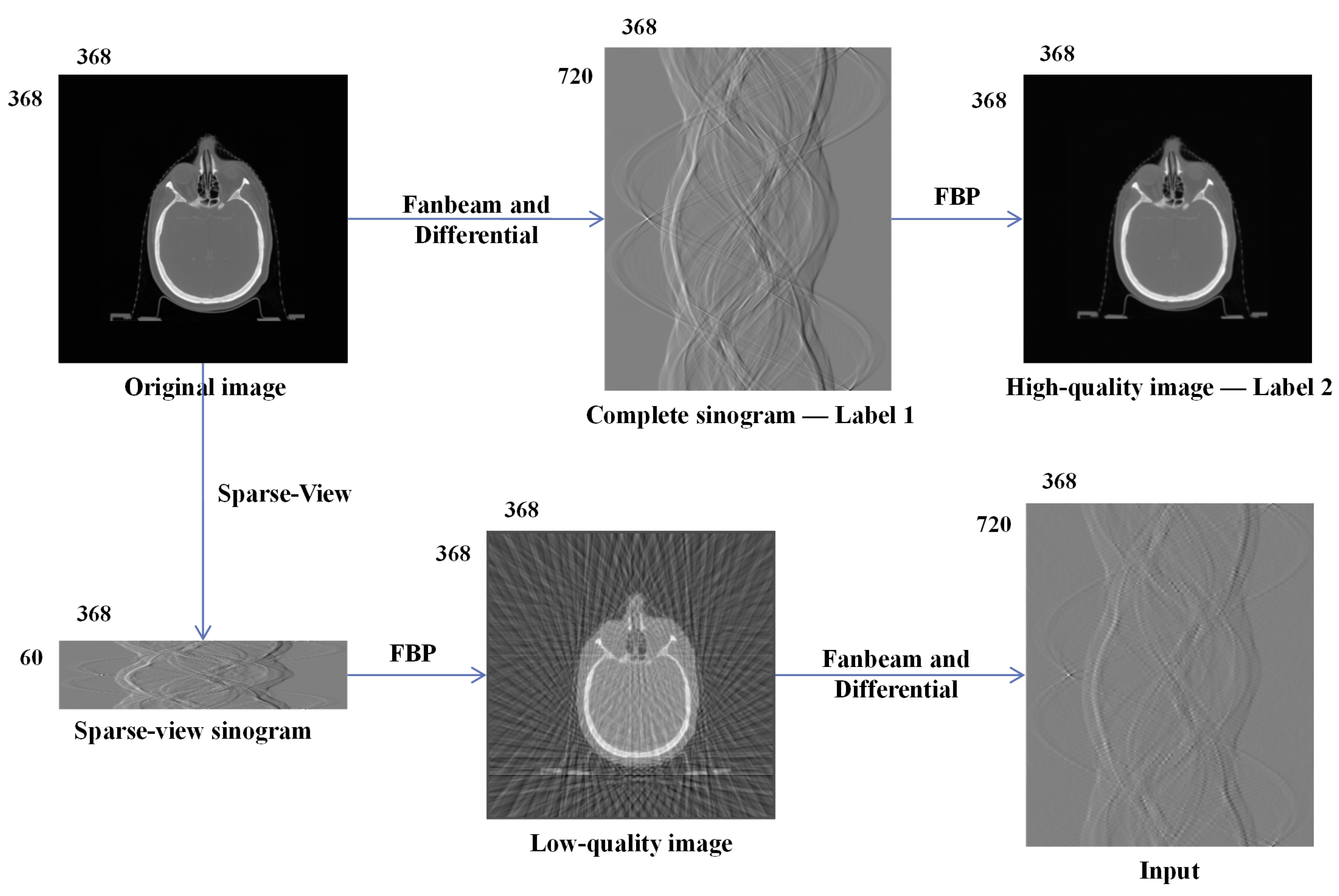
The simulated datasets are generated by performing the differential fan-beam forward projection operation to images in the head and neck CT image database of The Cancer Imaging Archive (TCIA) [42,43], as shown in Figure 2. TCIA is a large-scale open-access database that contains medical images of common tumors and the corresponding clinical information, such as magnetic resonance imaging (MRI), positron emission computed tomography (PET), and CT. While performing the differential forward projection operation, the sampling step is set to 0.5, 2, 3, 4, and 6 with complete scanning of 360 ° , corresponding to 720, 180, 120, 90, and 60 views, respectively. Projection sinograms with 720 views are considered as complete and others as sparse-view. The distance between the source and detector and that between the source and object are set to 20,000 and 18,000 pixels. The offset is set to 0.600 CT images from 30 patients, and a size of 368 × 368 pixels is used to generate the simulated datasets, where 400 CT images are used to train the network and 200 CT images to test the network. Each patient provides 20 CT images.
Specifically, the differential forward projection as expressed in Equations (3) and (4) of the mentioned sampling factors are performed on the phantoms, where complete projection sinograms are used as the labels of the enhanced network in the projection sinogram domain. The PCCT FBP reconstruction as expressed in Equations (1) and (2) is executed on these sinograms to obtain the reconstructed images, where the images reconstructed with complete projection sinograms are used as the labels of the enhanced network in the image domain. Finally, the differential forward projection of 720 views is performed on the degraded images reconstructed with sparse-view projection sinograms, and the results are used as the input of the network. In addition, the projection sinograms used in this network have a size of 720 × 368 pixels and the CT images 368 × 368 pixels.

3.1.2. Experimental

The experimental datasets were generated by performing the fan-beam PCCT experiments on the mouse paw, which was provided by Institute of High Energy Physics, Chinese Academy of Sciences. The used mouse was kept in a pathogen-free environment and was fed ad lib. The procedures for care and use of this mouse were conducted in accordance with the “Guiding Principles in the Care and Use of Animals” [44] and were approved by the Ethics Committee of the Institute of High Energy Physics, Chinese Academy of Sciences. While scanning, 720 views were acquired within 360 degrees using the laboratory fan-beam X-ray source to obtain complete projections. Four phase steppings occurred at each sampling view. Then, sparse sampling was carried out on the complete projections to obtain sparse-view projections with 180, 120, 90, and 60 views. The distances between the source and detector and that between the source and object were 22,400 and 20,200 pixels. The offset was four pixels. The acquired projection images had a size of 512 × 512 pixels, and the corresponding sinograms and reconstructed images had sizes of 720 × 512 and 512 × 512 pixels, respectively. In the experiments, 600 tomographic images were obtained, where the first 400 images from top to bottom were chosen for training and the remaining 200 images for testing.

3.2. Implementation

The proposed DDPC-Net was implemented by Python 3.5.2 and Tensorflow 1.8, and the Adam [45] optimizer with a mini-batch size of 2 was applied to train this framework. All the models were trained for 100 epochs on Nvidia GTX 1080Ti graphics processing unit (GPU).
Equations (11)–(13) present the loss function of this framework containing the penalties on the dual domains, where the subscripts 1 and 2 represent the projection sinogram domain and the image domain, and α and α ^ represent the learning result and the ground truth. The loss function in each domain is the same, composed of the weighted sum of the mean square error (MSE) and the multi-scale structure similarity (MS-SSIM). MSE helps to reduce the difference in pixel values, and MS-SSIM is closer to subjective quality evaluation methods. The learning rate gradually decreased from 1 × 10 4 to 1 × 10 6 while training.
l o s s = l o s s 1 + l o s s 2
l o s s 1 = M S E ( α 1 , α 1 ^ ) + 0.2 · ( 1 M S _ S S I M ( α 1 , α 1 ^ ) )
l o s s 2 = M S E ( α 2 , α 2 ^ ) + 0.2 · ( 1 M S _ S S I M ( α 2 , α 2 ^ ) )

3.3. Comparison Methods

Several existing DL-based CT approaches are used as comparisons for DDPC-Net, including the denseness-deconvolution network (DD-Net) [37], the DLFBP framework [34], and the hybrid domain neural network (HD-Net) [38], which respectively represent the enhanced network in the projection sinogram domain, the image domain, and the dual domains.

3.4. Image Evaluation

Image evaluation consisted of qualitative and quantitative evaluation. Qualitative evaluation was achieved by observing the reconstructed images and the regions of interest (ROI). The feature similarity (FSIM) and the information weighted SSIM (IW-SSIM) were used for quantitative evaluation, which outperforms other evaluation methods on accuracy [46].
In addition, the relative improvement ratios ( r e l I ) for the above two evaluation indexes are defined in Equation (14), where M F B P and M represent the image evaluation indexes of the results from FBP and other methods.
r e l I = M M F B P M F B P

3.5. Efficiency

The efficiency of the used deep learning methods was evaluated based on the number of parameters included in each framework and the runtime with the same epochs. The number of parameters was calculated by adding one of each layer in the network, as presented in Equation (16), where N l p represents the number of parameters in each layer, N i represents the number of input feature images, N o represents the number of output feature images, and f h and f w respectively represent the height and width of the convolutional filter. The runtime was obtained by subtracting the end time and start time.
N l p = ( N i × f h × f w + 1 ) × N o

3.6. Results

3.6.1. Simulation

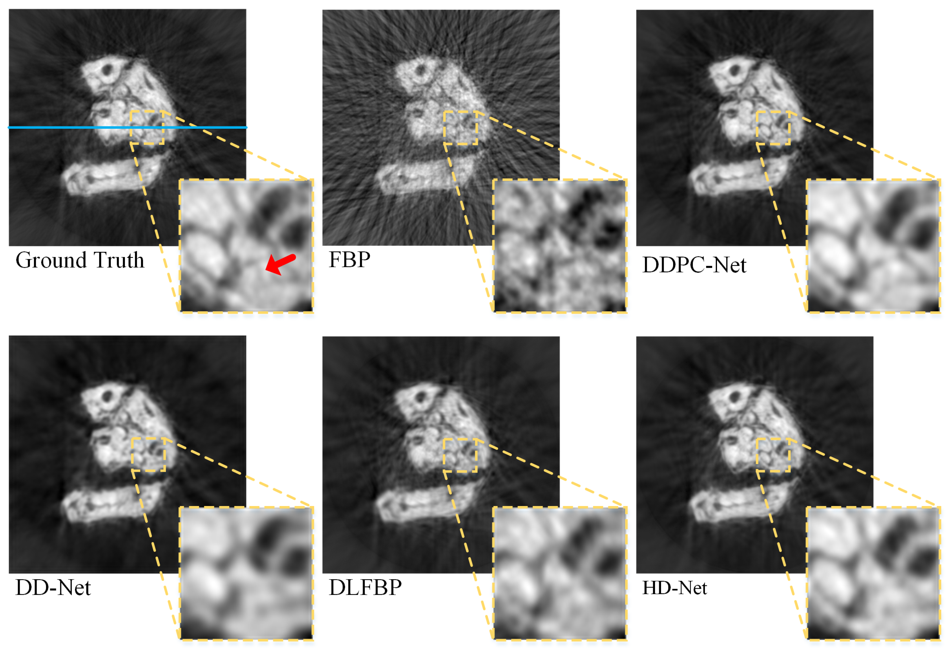
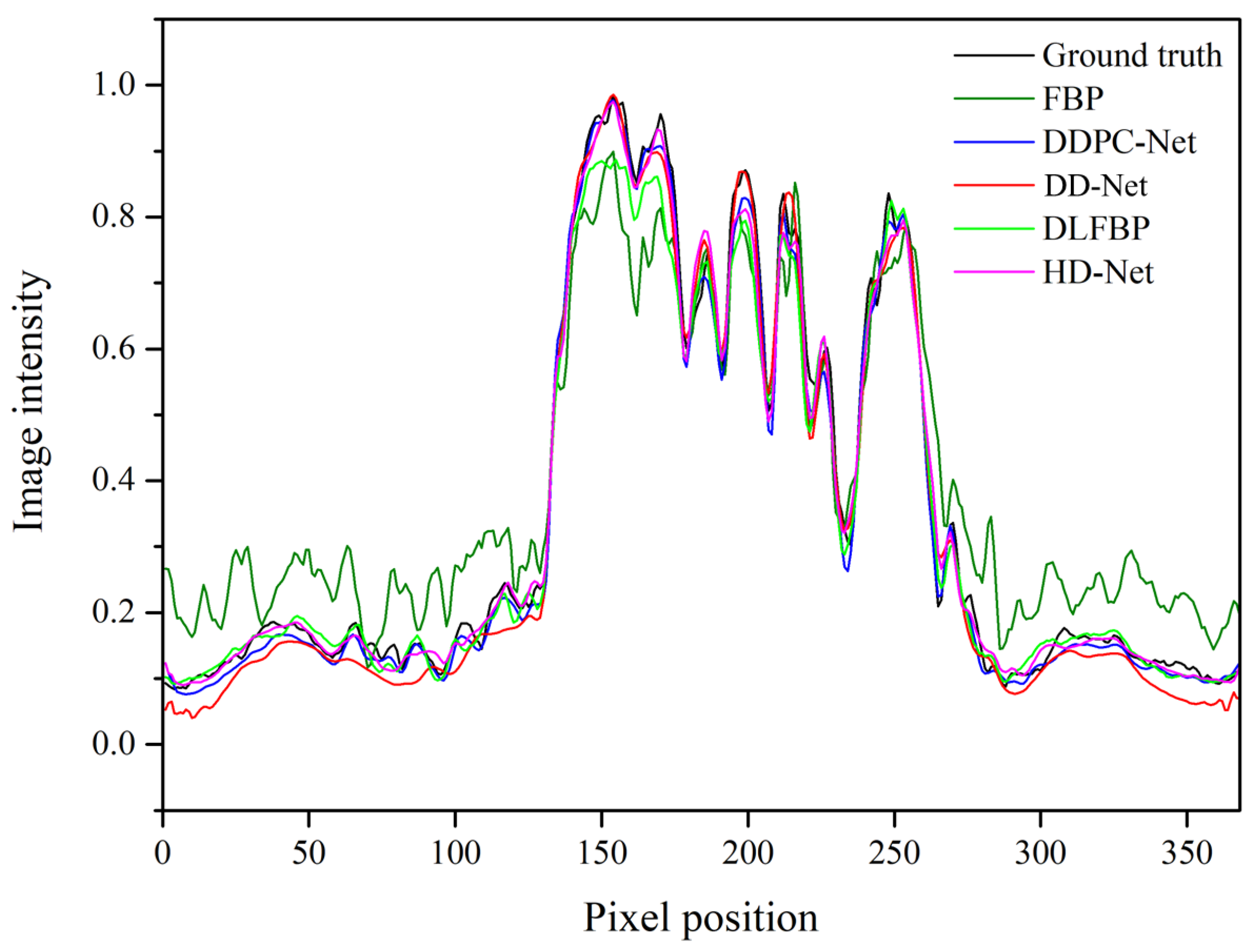
Figure 3 presents the results of the simulated testing datasets with 60 views. The ROI is indicated with the dashed square, which is enlarged and shown for better visualization. The image profiles along the blue line in Figure 3 are drawn and shown in Figure 4.
As expected, severe streak artifacts introduced by sparse-view sampling exist in FBP reconstruction and much less in the results of other methods. However, for DD-Net, the image is blurred, and some image structure still vanishes. For DLFBP, great unpredictable artifacts exist, which affect the visual observation of the image structure. HD-Net and DDPC-Net efficiently suppress artifacts and restore the vanished structure, while the result of HD-NET is a little more blurred compared with DDPC-Net. As presented in Figure 4, the intensity curves in the images from DLFBP and DDPC-Net are noticeably closer to the ground truth, while the intensity curve of DLFBP is relatively more undulating. Table 1 lists the FSIM and IW-SSIM values of the images in Figure 3. DDPC-Net achieves at least 5 % higher values in terms of FSIM and IW-SSIM, which support the conclusion of the visual observation.
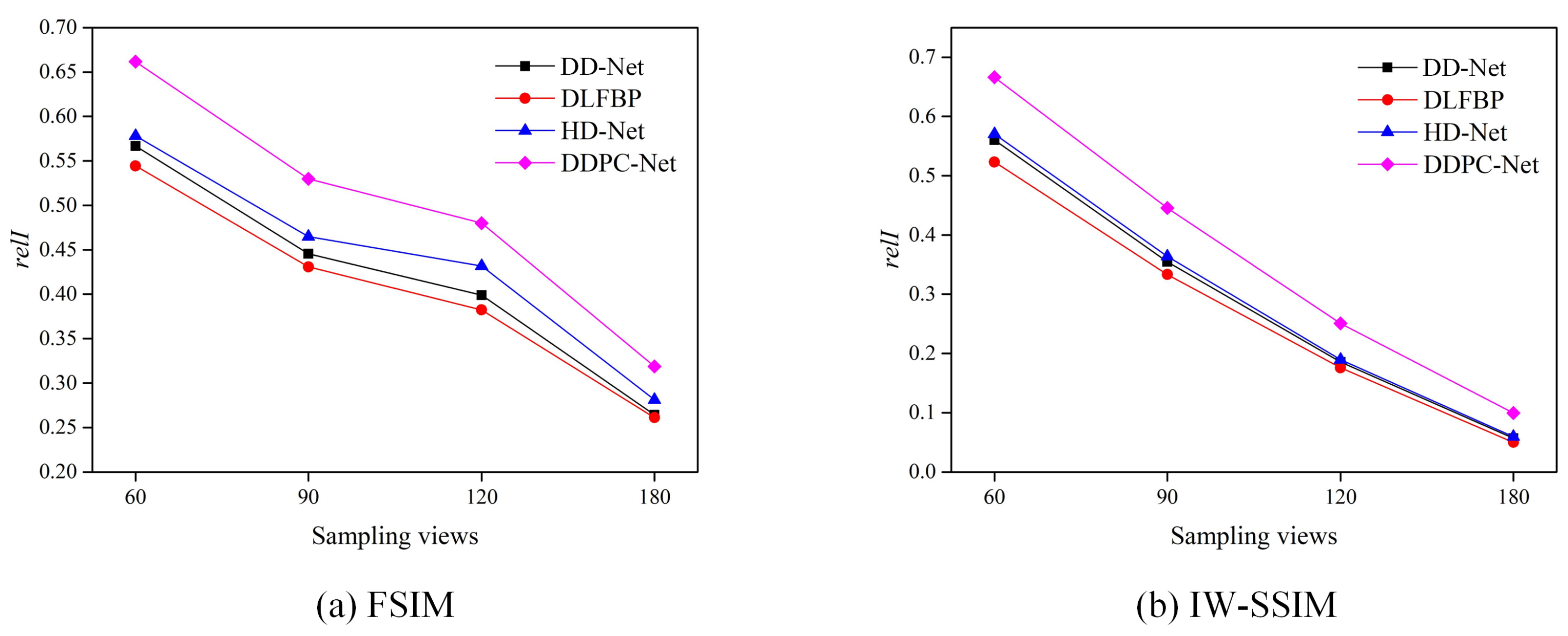
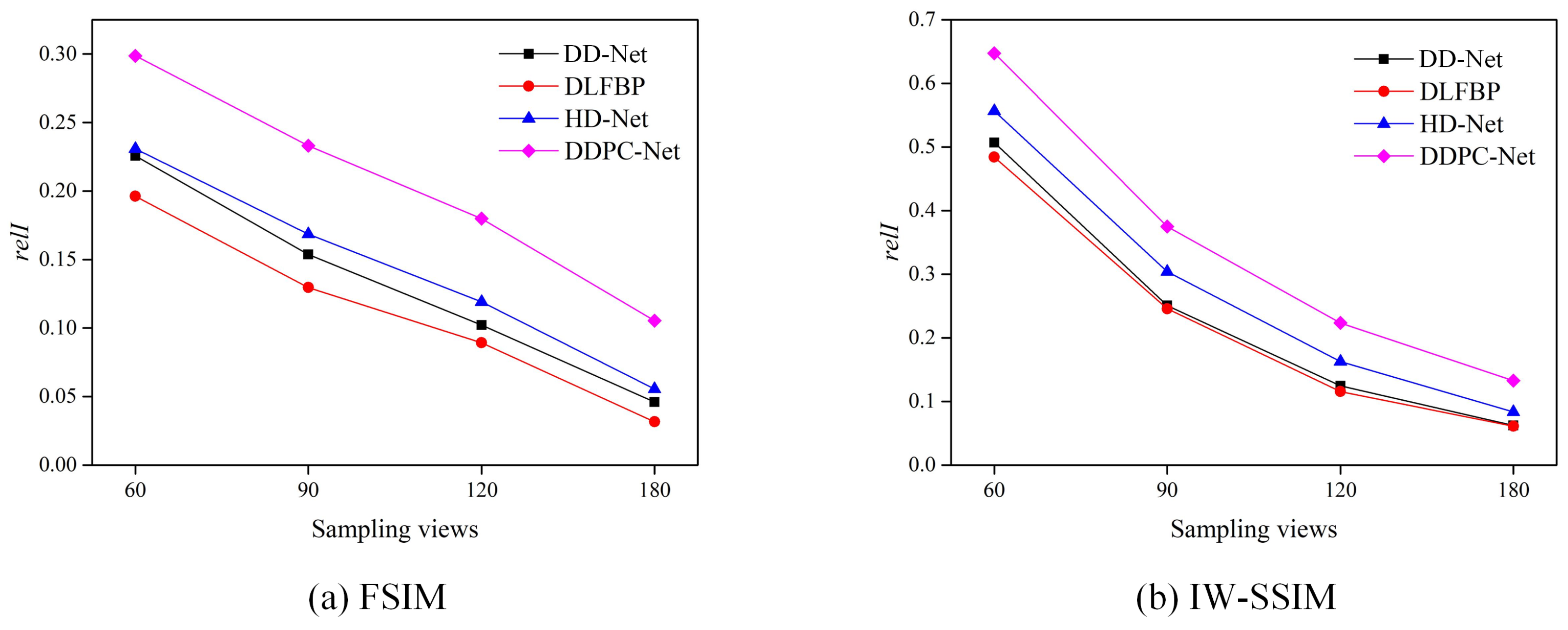
Table 2 lists the average FSIM and IW-SSIM values of the results of the mentioned five methods. It can be observed that as the number of sampling views increases, the average FSIM and IW-SSIM values increase, and the methods except for FBP obtain values higher than 90 % . In addition, DDPC-Net achieves slightly better values than the other methods. The r e l I of the average values of the average FSIM and IW-SSIM values are drawn in Figure 5. The same conclusion can be drawn that DDPC-Net outperforms other methods. Moreover, Figure 5 shows that the image quality of the results decreases drastically with the decrease in number of the sampling views. Table 3 lists the efficiency of the four deep learning methods. As expected, the efficiency of the dual-domain reconstruction frameworks is slightly lower than that of the single-domain reconstruction framework, both in terms of the number of parameters and runtime. However, compared to HD-Net, which trains enhancement networks in the projection sinogram domain and image domain separately and cascades them, DDPC-Net is more efficient. This indicates that the proposed method can balance image quality and efficiency.

3.6.2. Experimental

Figure 6 shows the results of the experimental testing datasets with 60 views. The ROI is indicated with the dashed square, which is enlarged and shown to obtain better visualization. The analysis of the experimental datasets was performed as the same as that of the simulation datasets. The corresponding curves and index values are presented in Figure 7 and Figure 8 and Table 4, Table 5 and Table 6. The same conclusion can be drawn as that of the simulation datasets. The images of DD-Net and HD-Net are blurred and lose some structure. There are severe artifacts existing in the images of DLFBP. Furthermore, DDPC-Net outperforms the comparison methods. In addition, the FSIM and IW-SSIM values of the experimental datasets are significantly worse than those of the simulation datasets, since noise introduced during the experiment degrades the experimental datasets.

4. Discussion

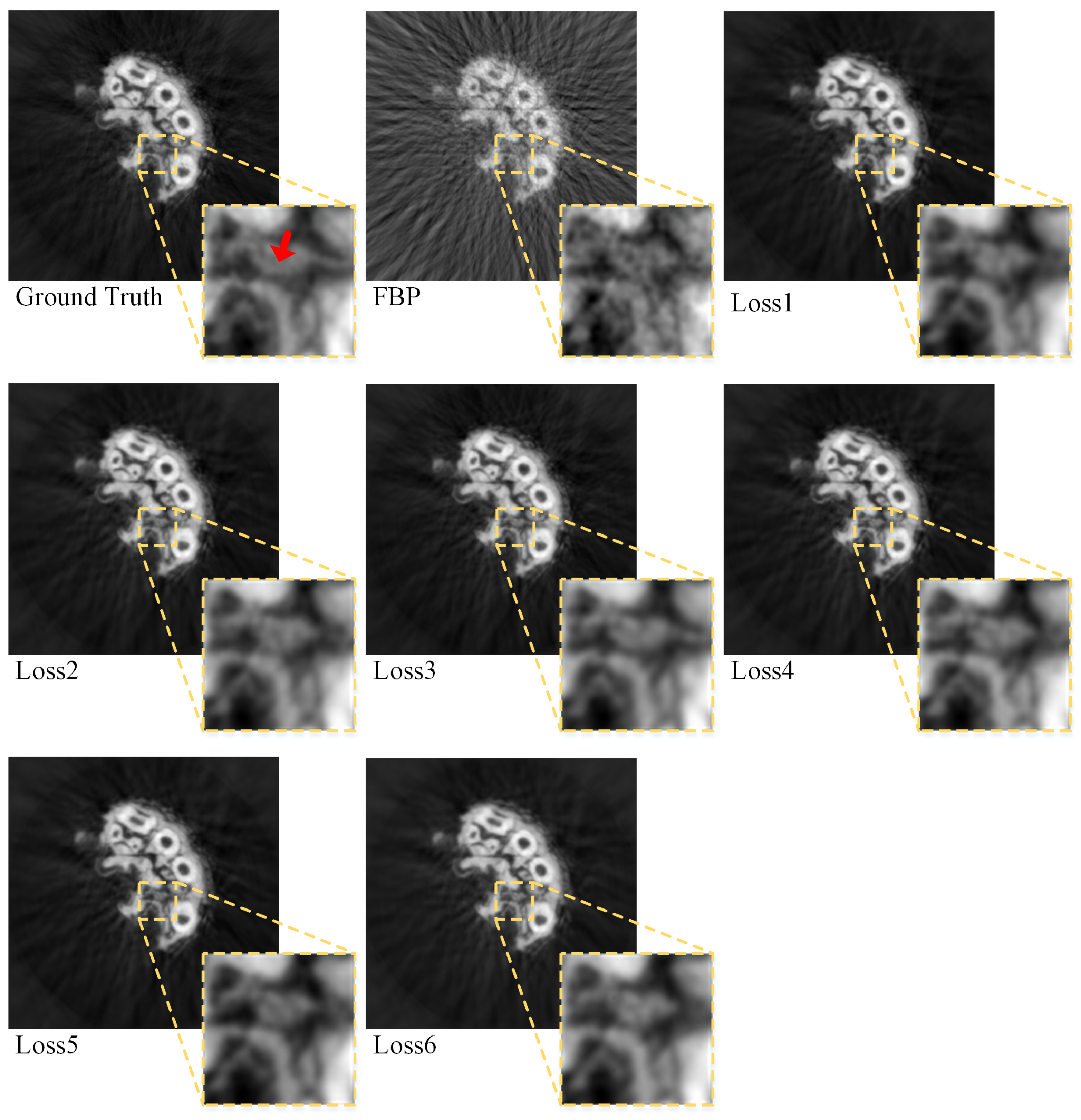
After the network architecture is determined, the loss function has a great effect on the results. In this work, the weighted sums of MSE and MS-SSIM are adopted as the loss function, as shown in Equation (16), where ω 1 and ω 2 represent the weight of MSE and MS-SSIM. ω 1 of 1 and ω 2 of 0.2 are adopted in the experiments. To discuss the influence of the weight values on the image quality and to validate that the best weight values are adopted, the experiments are repeated with different ω 1 and ω 2 . Considering the experimental datasets as examples, the network is trained with several commonly used loss functions (i.e., Loss1, Loss2, Loss3, Loss4, Loss5, and Loss6), as presented in Table 7.
l o s s = ω 1 M S E ( α , α ^ ) + ω 2 ( 1 M S _ S S I M ( α , α ^ ) )
Figure 9 shows one of the results of the experimental testing datasets with 60 views, and the ROI is indicated with a dashed square, which is enlarged and shown for better visualization. It can be observed that Loss2 and Loss3 help to obtain high-quality results, and the result with Loss3 has a relatively clearer structure. Table 8 lists the FSIM and IW-SSIM values of the images in Figure 9. These values provide evidence that the network trained with Loss3 outperforms those trained with other loss functions mentioned.
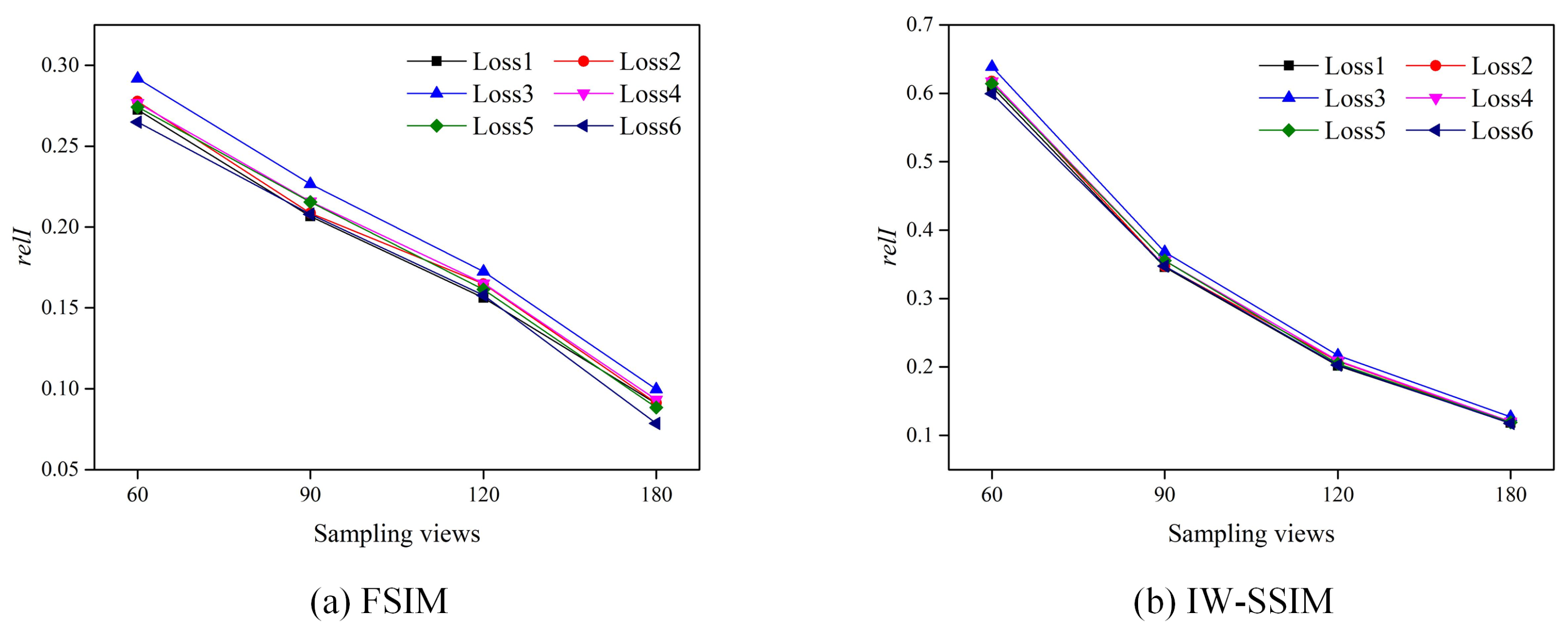
Table 9 lists the average FSIM and MS-SSIM values of the results with different loss functions. Figure 10 presents the r e l I of the average values of FSIM and IW-SIIM. Furthermore, regarding the number of the sampling view, DDPC-Net with Loss3 enables the best performance in imaging. It also indicates that the CNNs with a combination of several losses may outperform that with a single loss of the applications in the field of CT.

5. Conclusions

In this paper, we reported a DL reconstruction framework for PCCT with sparse-view projections and validated it with experiments of the simulation datasets and experimental datasets. The proposed framework consists of CNNs in dual domains and PCRIL as the connection between them. PCRIL can achieve PCCT reconstruction, and it allows for the backpropagation of gradients from the image domain to the projection sinogram domain. Therefore, this framework enables the CNNs in dual domains to be trained simultaneously for further reduction of artifacts and to restore the missing structure introduced by sparse-view sampling. In addition, the differential forward projection of the image reconstructed with the sparse-view projection sinogram is adopted as the input of the network, instead of the interpolation of the sparse-view projection sinogram. It efficiently improves the image quality of the images reconstructed with given sparse-view PCCT projections. This work has the potential to push PCCT techniques to applications in the field of composite imaging and biomedical imaging.

Author Contributions

Conceptualization, C.Z. and J.F.; methodology, C.Z. and J.F.; software, C.Z.; validation, C.Z. and J.F.; formal analysis, C.Z.; investigation, C.Z.; resources, J.F. and G.Z.; data curation, C.Z.; writing—original draft preparation, C.Z.; writing—review and editing, J.F. and G.Z.; visualization, C.Z.; supervision, J.F. and G.Z.; project administration, J.F. and G.Z.; funding acquisition, J.F. All authors have read and agreed to the published version of the manuscript.

Funding

This research was funded by the Ningbo Major Projects of Science and Technology Innovation 2025 (2020Z074), the National Natural Science Foundation of China (51975026), the Joint Fund of Research Utilizing Large-scale Scientific Facilities by the National Natural Science Foundation of China and Chinese Academy of Science (U1932111), the Innovation Leading Talent Short Term Projects of Natural Science by Jiangxi Double Thousand Plan (S2020DQKJ0355), the Jiangxi Provincial Science and Technology Innovation Base Plan—Introduction of workpiece research and development institutions (20203CCH45003), and the Jiangxi Provincial Science and Technology Innovation Base Plan—Introduction of workpiece research and development institutions (20212CCH45001).

Institutional Review Board Statement

The procedures for care and use of the used mouse were conducted in accordance with the “Guiding Principles in the Care and Use of Animals” and were approved by the Ethics Committee of the Institute of High Energy Physics, Chinese Academy of Sciences.

Informed Consent Statement

Not applicable.

Data Availability Statement

Data was obtained from the Institute of High Energy Physics, Chinese Academy of Sciences and are available from J.F. with the permission of the Institute of High Energy Physics, Chinese Academy of Sciences.

Acknowledgments

The authors are grateful to Peiping Zhu (Institute of High Energy Physics, Chinese Academy of Sciences) for providing us the experimental datasets.

Conflicts of Interest

The authors declare no conflict of interest.

References

  1. Venkatesh, E.; Elluru, S.V. Cone beam computed tomography: Basics and applications in dentistry. J. Istanb. Univ. Fac. Dent. 2017, 51, S102. [Google Scholar] [CrossRef]
  2. Ardila, D.; Kiraly, A.P.; Bharadwaj, S.; Choi, B.; Reicher, J.J.; Peng, L.; Tse, D.; Etemadi, M.; Ye, W.; Corrado, G.; et al. End-to-end lung cancer screening with three-dimensional deep learning on low-dose chest computed tomography. Nat. Med. 2019, 25, 954–961. [Google Scholar] [CrossRef]
  3. Zhu, T.; Wang, Y.; Zhou, S.; Zhang, N.; Xia, L. A comparative study of chest computed tomography features in young and older adults with corona virus disease (COVID-19). J. Thorac. Imaging 2020, 35, W97. [Google Scholar] [CrossRef] [PubMed]
  4. Li, W.; Cui, H.; Li, K.; Fang, Y.; Li, S. Chest computed tomography in children with COVID-19 respiratory infection. Pediatr. Radiol. 2020, 50, 796–799. [Google Scholar] [CrossRef] [PubMed]
  5. Du Plessis, A.; Rossouw, P. X-ray computed tomography of a titanium aerospace investment casting. Case Stud. Nondestruct. Test. Eval. 2015, 3, 21–26. [Google Scholar] [CrossRef]
  6. Thompson, A.; Maskery, I.; Leach, R.K. X-ray computed tomography for additive manufacturing: A review. Meas. Sci. Technol. 2016, 27, 072001. [Google Scholar] [CrossRef]
  7. Asadizanjani, N.; Tehranipoor, M.; Forte, D. PCB reverse engineering using nondestructive X-ray tomography and advanced image processing. IEEE Trans. Components Packag. Manuf. Technol. 2017, 7, 292–299. [Google Scholar] [CrossRef]
  8. Townsend, A.; Pagani, L.; Scott, P.; Blunt, L. Areal surface texture data extraction from X-ray computed tomography reconstructions of metal additively manufactured parts. Precis. Eng. 2017, 48, 254–264. [Google Scholar] [CrossRef]
  9. Bonse, U.; Hart, M. An X-ray interferometer with Bragg case beam splitting and beam recombination. Z. Phys. 1966, 194, 1–17. [Google Scholar] [CrossRef]
  10. Ingal, V.; Beliaevskaya, E. X-ray plane-wave topography observation of the phase contrast from a non-crystalline object. J. Phys. D Appl. Phys. 1995, 28, 2314. [Google Scholar] [CrossRef]
  11. Wilkins, S.; Gureyev, T.E.; Gao, D.; Pogany, A.; Stevenson, A. Phase-contrast imaging using polychromatic hard X-rays. Nature 1996, 384, 335–338. [Google Scholar] [CrossRef]
  12. Nugent, K.; Gureyev, T.; Cookson, D.; Paganin, D.; Barnea, Z. Quantitative phase imaging using hard X-rays. Phys. Rev. Lett. 1996, 77, 2961. [Google Scholar] [CrossRef] [PubMed]
  13. Weitkamp, T.; Diaz, A.; David, C.; Pfeiffer, F.; Stampanoni, M.; Cloetens, P.; Ziegler, E. X-ray phase imaging with a grating interferometer. Opt. Express 2005, 13, 6296–6304. [Google Scholar] [CrossRef]
  14. Pfeiffer, F.; Weitkamp, T.; Bunk, O.; David, C. Phase retrieval and differential phase-contrast imaging with low-brilliance X-ray sources. Nat. Phys. 2006, 2, 258–261. [Google Scholar] [CrossRef]
  15. Cloetens, P.; Ludwig, W.; Baruchel, J.; Van Dyck, D.; Van Landuyt, J.; Guigay, J.; Schlenker, M. Holotomography: Quantitative phase tomography with micrometer resolution using hard synchrotron radiation X-rays. Appl. Phys. Lett. 1999, 75, 2912–2914. [Google Scholar] [CrossRef]
  16. Bech, M.; Jensen, T.H.; Feidenhans, R.; Bunk, O.; David, C.; Pfeiffer, F. Soft-tissue phase-contrast tomography with an X-ray tube source. Phys. Med. Biol. 2009, 54, 2747. [Google Scholar] [CrossRef]
  17. Donath, T.; Pfeiffer, F.; Bunk, O.; Grünzweig, C.; Hempel, E.; Popescu, S.; Vock, P.; David, C. Toward clinical X-ray phase-contrast CT: Demonstration of enhanced soft-tissue contrast in human specimen. Investig. Radiol. 2010, 45, 445–452. [Google Scholar] [CrossRef] [PubMed]
  18. Momose, A.; Takeda, T.; Itai, Y.; Hirano, K. Phase–contrast X–ray computed tomography for observing biological soft tissues. Nat. Med. 1996, 2, 473–475. [Google Scholar] [CrossRef] [PubMed]
  19. Zhu, P.; Zhang, K.; Wang, Z.; Liu, Y.; Liu, X.; Wu, Z.; McDonald, S.A.; Marone, F.; Stampanoni, M. Low-dose, simple, and fast grating-based X-ray phase-contrast imaging. Proc. Natl. Acad. Sci. USA 2010, 107, 13576–13581. [Google Scholar] [CrossRef] [PubMed]
  20. Ge, Y.; Li, K.; Garrett, J.; Chen, G.H. Grating based X-ray differential phase contrast imaging without mechanical phase stepping. Opt. Express 2014, 22, 14246–14252. [Google Scholar] [CrossRef] [PubMed]
  21. Quan, Y.; Chen, Y.; Shao, Y.; Teng, H.; Xu, Y.; Ji, H. Image denoising using complex-valued deep CNN. Pattern Recognit. 2021, 111, 107639. [Google Scholar] [CrossRef]
  22. Zhu, H.; Xie, C.; Fei, Y.; Tao, H. Attention mechanisms in CNN-based single image super-resolution: A brief review and a new perspective. Electronics 2021, 10, 1187. [Google Scholar] [CrossRef]
  23. Nguyen, Q.H.; Nguyen, B.P.; Nguyen, T.B.; Do, T.T.; Mbinta, J.F.; Simpson, C.R. Stacking segment-based CNN with SVM for recognition of atrial fibrillation from single-lead ECG recordings. Biomed. Signal Process. Control. 2021, 68, 102672. [Google Scholar] [CrossRef]
  24. Zhou, W.; Liu, M.; Xu, Z. The dual-fuzzy convolutional neural network to deal with handwritten image recognition. IEEE Trans. Fuzzy Syst. 2022, 30, 5225–5236. [Google Scholar] [CrossRef]
  25. Lu, J.; Tan, L.; Jiang, H. Review on convolutional neural network (CNN) applied to plant leaf disease classification. Agriculture 2021, 11, 707. [Google Scholar] [CrossRef]
  26. Yu, J.; Fan, Y.; Yang, J.; Xu, N.; Wang, Z.; Wang, X.; Huang, T. Wide activation for efficient and accurate image super-resolution. arXiv 2018, arXiv:1808.08718. [Google Scholar]
  27. Wang, J.; Liang, J.; Cheng, J.; Guo, Y.; Zeng, L. Deep learning based image reconstruction algorithm for limited-angle translational computed tomography. PLoS ONE 2020, 15, e0226963. [Google Scholar]
  28. Han, Y.; Wu, D.; Kim, K.; Li, Q. End-to-end deep learning for interior tomography with low-dose X-ray CT. Phys. Med. Biol. 2022, 67, 115001. [Google Scholar] [CrossRef]
  29. Liu, Y.; Kang, J.; Li, Z.; Zhang, Q.; Gui, Z. Low-dose CT noise reduction based on local total variation and improved wavelet residual CNN. J. X-ray Sci. Technol. 2022, 30, 1229–1242. [Google Scholar] [CrossRef] [PubMed]
  30. Lee, H.; Lee, J.; Cho, S. View-interpolation of sparsely sampled sinogram using convolutional neural network. In Proceedings of the Medical Imaging 2017: Image Processing; International Society for Optics and Photonics: San Diego, CA, USA, 2017; Volume 10133, p. 1013328. [Google Scholar]
  31. Ronneberger, O.; Fischer, P.; Brox, T. U-net: Convolutional networks for biomedical image segmentation. In Proceedings of the International Conference on Medical Image Computing and Computer-Assisted Intervention, Munich, Germany, 5–9 October 2015; pp. 234–241. [Google Scholar]
  32. He, K.; Zhang, X.; Ren, S.; Sun, J. Deep residual learning for image recognition. In Proceedings of the IEEE Conference on Computer Vision and Pattern Recognition, Las Vegas, NV, USA, 27–30 June 2016; pp. 770–778. [Google Scholar]
  33. Lee, H.; Lee, J.; Kim, H.; Cho, B.; Cho, S. Deep-neural-network-based sinogram synthesis for sparse-view CT image reconstruction. IEEE Trans. Radiat. Plasma Med. Sci. 2018, 3, 109–119. [Google Scholar] [CrossRef]
  34. Fu, J.; Dong, J.; Zhao, F. A deep learning reconstruction framework for differential phase-contrast computed tomography with incomplete data. IEEE Trans. Image Process. 2019, 29, 2190–2202. [Google Scholar] [CrossRef] [PubMed]
  35. Chen, H.; Zhang, Y.; Kalra, M.K.; Lin, F.; Chen, Y.; Liao, P.; Zhou, J.; Wang, G. Low-dose CT with a residual encoder-decoder convolutional neural network. IEEE Trans. Med. Imaging 2017, 36, 2524–2535. [Google Scholar] [CrossRef] [PubMed]
  36. Kang, E.; Min, J.; Ye, J.C. A deep convolutional neural network using directional wavelets for low-dose X-ray CT reconstruction. Med. Phys. 2017, 44, e360–e375. [Google Scholar] [CrossRef] [PubMed]
  37. Zhang, Z.; Liang, X.; Dong, X.; Xie, Y.; Cao, G. A sparse-view CT reconstruction method based on combination of DenseNet and deconvolution. IEEE Trans. Med. Imaging 2018, 37, 1407–1417. [Google Scholar] [CrossRef] [PubMed]
  38. Hu, D.; Liu, J.; Lv, T.; Zhao, Q.; Zhang, Y.; Quan, G.; Feng, J.; Chen, Y.; Luo, L. Hybrid-Domain Neural Network Processing for Sparse-View CT Reconstruction. IEEE Trans. Radiat. Plasma Med. Sci. 2020, 5, 88–98. [Google Scholar] [CrossRef]
  39. Lee, D.; Choi, S.; Kim, H.J. High quality imaging from sparsely sampled computed tomography data with deep learning and wavelet transform in various domains. Med. Phys. 2019, 46, 104–115. [Google Scholar] [CrossRef]
  40. Lin, W.A.; Liao, H.; Peng, C.; Sun, X.; Zhang, J.; Luo, J.; Chellappa, R.; Zhou, S.K. Dudonet: Dual domain network for ct metal artifact reduction. In Proceedings of the IEEE/CVF Conference on Computer Vision and Pattern Recognition, Long Beach, CA, USA, 15–20 June 2019; pp. 10512–10521. [Google Scholar]
  41. Pfeiffer, F.; Kottler, C.; Bunk, O.; David, C. Hard X-ray phase tomography with low-brilliance sources. Phys. Rev. Lett. 2007, 98, 108105. [Google Scholar] [CrossRef] [PubMed]
  42. Lai, H.; Chen, W.; Fu, H. A new double-sampling method for mediastinal lymph nodes detection by deep conventional neural network. In Proceedings of the 2018 Chinese Control And Decision Conference (CCDC), Shenyang, China, 9–11 June 2018; pp. 6286–6290. [Google Scholar]
  43. Seff, A.; Lu, L.; Cherry, K.M.; Roth, H.R.; Liu, J.; Wang, S.; Hoffman, J.; Turkbey, E.B.; Summers, R.M. 2D view aggregation for lymph node detection using a shallow hierarchy of linear classifiers. In Proceedings of the International Conference on Medical image Computing and Computer-Assisted Intervention, Boston, MA, USA, 14–18 September 2014; pp. 544–552. [Google Scholar]
  44. Guidelines for the Ethical Review of Laboratory Animal Welfare (GB/T 35892-2018). Standardization Administration of China Beijing ICP 09001239. Available online: http://www.gb688.cn/bzgk/gb/newGbInfo?hcno=9BA619057D5C13103622A10FF4BA5D14 (accessed on 20 March 2022).
  45. Aerts, H.J.; Velazquez, E.R.; Leijenaar, R.T.; Parmar, C.; Grossmann, P.; Carvalho, S.; Bussink, J.; Monshouwer, R.; Haibe-Kains, B.; Rietveld, D.; et al. Decoding tumour phenotype by noninvasive imaging using a quantitative radiomics approach. Nat. Commun. 2014, 5, 4006. [Google Scholar] [CrossRef] [PubMed]
  46. Zhang, L.; Zhang, L.; Mou, X.; Zhang, D. A comprehensive evaluation of full reference image quality assessment algorithms. In Proceedings of the 2012 19th IEEE International Conference on Image Processing, Orlando, FL, USA, 30 September–3 October 2012; pp. 1477–1480. [Google Scholar]
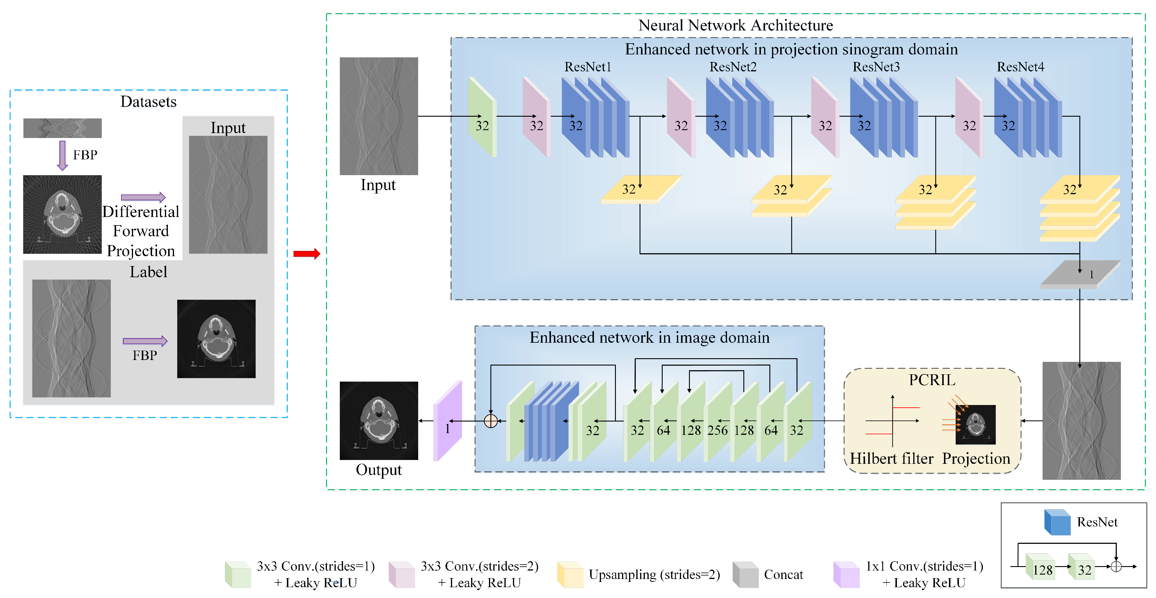
Figure 1. The architecture of the proposed DL framework for PCCT. It consists of the FBP algorithm for PCCT, the differential forward projection operation, and the neural network that allows the network parameters in dual domains to be synchronously updated.
Applsci 13 06051 g001
Figure 2. The data preparation process of the simulated datasets.
Applsci 13 06051 g002
Figure 3. The reconstructed images of one of the results of the simulated testing datasets. This sinogram has 60 sampling views, and the reconstructed images were obtained by five methods.
Applsci 13 06051 g003
Figure 4. The profiles along the blue solid line in Figure 3.
Applsci 13 06051 g004
Figure 5. The relI curves of the average values of FSIM and IW-SSIM of the simulated testing datasets.
Applsci 13 06051 g005
Figure 6. The reconstructed images of the results of the experimental testing datasets. This sinogram has 60 sampling views, and the reconstructed images were obtained by five methods.
Applsci 13 06051 g006
Figure 7. The profiles along the blue solid line in Figure 5.
Applsci 13 06051 g007
Figure 8. The relI curves of the average values of FSIM and IW-SSIM of the experimental testing datasets.
Applsci 13 06051 g008
Figure 9. The reconstructed images of one of the results of the experimental testing datasets with different loss functions. This sinogram has 60 sampling views, and the reconstructed images are obtained by DDPC-Net with loss functions as presented in Table 7.
Applsci 13 06051 g009
Figure 10. The relI curves of the average values of FSIM and IW-SSIM of the experimental testing datasets with loss functions as presented in Table 7.
Applsci 13 06051 g010
Table 1. The FSIM and IW-SSIM values of the images in Figure 3.
EvaluationFBPDD-NetDLFBPHD-NetDDPC-Net
FSIM0.56320.89220.87800.91530.9652
IW-SSIM0.56730.92780.89220.93000.9793
Table 2. The average values of FSIM and IW-SSIM for the results of the simulated testing datasets.
EvaluationMethodsCases
6090120180
FSIMFBP0.58510.63870.66710.7495
DD-Net0.91680.92340.93330.9475
DLFBP0.90370.91390.92210.9432
HD-Net0.92340.93570.95520.9604
DDPC-Net0.97220.97720.98740.9884
IW-SSIMFBP0.58790.68310.79610.9074
DD-Net0.91740.92540.94390.9589
DLFBP0.89550.91090.93600.9528
HD-Net0.92330.93180.94700.9616
DDPC-Net0.97950.98760.99570.9978
Table 3. The efficiency of the used methods with simulated datasets.
EfficiencyDD-NetDLFBPHD-NetDDPC-Net
Parameters (million)1.061.364.143.28
Runtime (s)0.170.210.470.41
Table 4. The FSIM and IW-SSIM values of the images in Figure 6.
EvaluationFBPDD-NetDLFBPHD-NetDDPC-Net
FSIM0.72720.89570.87510.90260.9584
IW-SSIM0.59570.88440.87500.91680.9690
Table 5. The average values of FSIM and IW-SSIM of the results of the experimental testing datasets.
EvaluationMethodsCases
6090120180
FSIMFBP0.72790.77560.81720.8858
DD-Net0.89220.89790.90060.9265
DLFBP0.87070.88410.89010.9138
HD-Net0.89590.90630.91450.9350
DDPC-Net0.94530.95640.96420.9791
IW-SSIMFBP0.58120.70520.79940.8753
DD-Net0.87580.88200.89880.9299
DLFBP0.86260.87840.89170.9287
HD-Net0.90470.91960.92940.9482
DDPC-Net0.95740.96970.97790.9915
Table 6. The efficiency of the used methods with experimental datasets.
EfficiencyDD-NetDLFBPHD-NetDDPC-Net
Parameters (million)1.462.045.914.48
Runtime (s)0.220.290.610.52
Table 7. The weight values of loss functions used in this work.
WeightLoss1Loss2Loss3Loss4Loss5Loss6
ω 1 111110
ω 2 00.10.20.511
Table 8. The weight values of loss functions used in this work.
EvaluationLoss1Loss2Loss3Loss4Loss5Loss6
FSIM0.93010.93480.95090.93400.93390.9270
IW-SSIM0.95310.95730.96760.95580.95350.9458
Table 9. The average values of FSIM and IW-SSIM of the results of the experimental testing datasets.
EvaluationMethodsCases
6090120180
FSIMLoss10.92620.93590.94480.9662
Loss20.93000.93740.95200.9666
Loss30.94030.95140.95820.9741
Loss40.92930.94300.95220.9684
Loss50.92750.94270.94910.9642
Loss60.92070.93690.94620.9554
IW-SSIMLoss10.93530.94920.96060.9789
Loss20.94020.95010.96620.9797
Loss30.95240.96470.97290.9866
Loss40.94000.95600.96670.9806
Loss50.93820.95610.96320.9796
Loss60.92950.95020.96150.9782
Disclaimer/Publisher’s Note: The statements, opinions and data contained in all publications are solely those of the individual author(s) and contributor(s) and not of MDPI and/or the editor(s). MDPI and/or the editor(s) disclaim responsibility for any injury to people or property resulting from any ideas, methods, instructions or products referred to in the content.