Causality Analysis with Different Probabilistic Distributions Using Transfer Entropy

Abstract

This paper presents the results of an analysis of causality detection in a multi-loop control system. The investigation focuses on application of the Transfer Entropy method, which is not commonly used during the exact construction of information and material flow pathways in the field of automation. Calculations are performed on simulated multi-loop control system data obtained from a system with a structure known a priori. The model incorporates the possibility of freely changing its parameters and of applying noise with different properties. In addition, a method for determining the entropy transfer between process variables is investigated. The fitting of different variants of the probability distribution functions to the data is crucial for effective evaluation of the Transfer Entropy approach. The obtained results allow for suggestions to be formulated with respect to choosing which probability function the transfer entropy should be based upon. Moreover, we provide a proposal for the design of a causality analysis approach that can reliably obtain information relationships.

1. Introduction

In recent years, the field of causality has experienced significant development in its fundamental and theoretical aspects as well as in various applications. Nevertheless, it is uncommon to make a distinction, as suggested by [1], between two prominent problem areas within the field. The first problem area concerns evaluating the probable effects of interventions that have been applied or are being considered. This is known as the “Effects of Causes” (EoC) problem. The second problem area involves determining whether an observed outcome in an individual case was caused by a prior intervention or exposure. This is referred to as the “Causes of Effects” (CoE) problem.

These considerations mainly concern the humanities, in particular philosophy [2]. With growing interest in the subject, research has moved to other areas of interest, e.g., education [3], medical science [4], economics [5], epidemiology [6], meteorology [7], and even environmental health [8]. While the engineering sciences are not omitted, here the nature of causality is understood in a different way. The purpose of such analysis is to find the cause, in the sense of the root cause error (or fault), while the phenomenon of the ”effect” is known or predicted using other available methods. In engineering applications, causality is always accompanied by the concept of relationships. No analysis would make sense without data generated artificially (simulations) or obtained from industrial plants (processes). The second case deals with very complex systems, resulting in a huge amount of collected data or observations.

It is important to be aware that control engineers understand the subject of causality in a specific narrow sense that is very close to the task of fault detection and diagnosis, which is a very popular aspect. On this basis, we may distinguish the mainstream research on fault detection (or groups of faults), in which the task of determining the cause seems to be a secondary issue. Moreover, the majority of existing approaches use the flow structure of the process, which can be obtained in two ways: first, by available process knowledge and modeling, and second, by data-based causality models [9]. From this perspective, causality analysis can provide support for fault detection. Multi-loop control systems generate another challenge, which is witnessed not by maintenance teams but by control engineering or daily operations staff. In cases where it is necessary to tune a multi-loop system, it is crucial to know which loop is the so-called problem generator that causes poor performance for itself and degrades other loops as a consequence. In such a case, control engineers must find that particular loop (the cause) in order to avoid the need to tune other loops. Similar challenges appear in case of alarm systems. In the case of an alarm, the operator is quite often overwhelmed by a cascade of successive derivative alarms. To recover the situation, it becomes necessary to dig into the cause. From this perspective, causality analysis may help in the design of so-called intelligent alarm management systems [10]. This paper addresses the first challenge, i.e., poor control propagation and cause detection.

Over the years, many experimental methods have been developed to deal with this issue. They can be generally divided into those requiring a model of the tested object and the so-called model-free approaches. In practice, in root cause analysis the appropriate method should be selected carefully based on process dynamics, the available data, and the type of error. In the literature, there may be found many examples of often conditional solutions, i.e., Granger causality and its extensions [11], cross-correlation analysis [12], information-theoretical methods [13], frequency domain methods [14], and Bayesian nets [15], and it is important to consider which of these methods are sufficient.

The Transfer Entropy (TE) method [16] is a model-free approach, which means it does not require a mathematical model. It has been used in simple simulation (theoretical) applications in its basic version [17] and a few applications of TE in the domain of causal analysis for industrial processes [18]. TE has been extensively applied to real-world objects in other domains, e.g., climate research, finance, neuroscience, and more. A distinction can be drawn between two separate approaches: the assumed Probabilistic Density Function (PDF) may be explicitly provided; alternatively, a non-parametric model of the distribution-like histogram or more advanced estimators relying on fixed binning with ranking, kernel density estimation, or the Darbellay–Vajda approach [19] can be used. Previous papers have presented estimators differing from the classic approach [20,21] as well as statistical tests implemented in modern toolboxes [22,23]. The possibility of using alternative estimators is a separate task, and is not developed in this study. Preliminary analysis for this subject has already been addressed [24], and it is obvious that this subject requires further attention. The topic shows the enormous potential of the chosen method in this case. Combined with the multithreading associated with data analysis [25], the conducted research sheds light on its hitherto unconsidered possibilities.

The considered research addresses the Gaussian probability density function. Few studies have been carried out on other distributions or on the impact of the consequent change in the quality of the obtained results [26]. This study uses data from a simulation model to determine the relationship between the variables, using the TE method with variant probability distributions.

The rest of this paper is organized as follows. Section 2 presents the Transfer Entropy approach (Section 2.1) and discusses the basic properties of the distributions selected for calculations (Section 2.2). Section 3 describes the simulation system used in this paper. Section 4 contains the calculation results for the generated simulation data, based on the selected distributions after evaluating the quality of fit for each of them. The results for the Gaussian distribution method are referenced in the same section. Finally, Section 5 contains the formulated suggestions and conclusions on the design of causality analysis with Transfer Entropy to obtain reliable information relationships.

2. Mathematical Modeling

This section presents required mathematical formulations that are used throughout the paper. Transfer Entropy (TE) is presented first, followed by the formulations used for the probabilistic density functions.

2.1. Transfer Entropy

Transfer Entropy provides an information-theoretic interpretation of Wiener’s definition of causality. Essentially, it quantifies the amount of information transferred from one variable to another by calculating the reduction in uncertainty when predictability is assumed [27]. It can be expressed by Equation (1):

$$T_{x\to y}=\sum _{y_{i+h},Y_i,X_j}p(y_{i+h},Y_i,X_j)·\frac{p\left(y_{i+h}\right|Y_i,X_j)}{p\left(y_{i+h}\right|Y_i)},$$

(1)

where the variable $Y_i=[y_i,y_{i-\tau },\dots ,y_{i-(l-1)\tau }]$, the variable $X_j=[x_j,x_{j-\tau },\dots ,x_{j-(k-1)\tau }]$, l and k are dimensional delay embedding vectors, p is defined as a complete or conditional Probability Density Function, $\tau$ represents sampling, and h denotes the prediction horizon. Transfer Entropy (TE) provides valuable information about causality without requiring delayed information. It measures the difference between information obtained from the simultaneous observation of past values of both x and y, and information obtained from the past values of x alone regarding a future observation of x [28].

To implement the Transfer Entropy approach between two variables, it is necessary to simplify the formula in Equation (1) to the form presented in Equation (2). This simplified form is used in practical applications.

$$T_{x\to y}=\sum _{y_i,y_{i-t},x_{i-\tau }}p(y_i,y_{i-t},x_{i-\tau })·\frac{p(y_i,y_{i-t},x_{i-\tau })p\left(y_{i-t}\right)}{p(y_{i-t},x_{i-\tau })p(y_i,y_{i-t})}.$$

(2)

The formula for Transfer Entropy involves a conditional Probability Density Function (PDF), denoted by p. The time lags in x and y are represented by $\tau$ and t, respectively. For this type of analysis, the probability density is typically estimated using a Gaussian density estimation method. If the time series is short, t is set to 1 based on the assumption that the datapoint immediately preceding the target value in y provides the maximum auto-transference of information.

Transfer Entropy is inherently asymmetric and is based on transition probabilities, making it a natural method for incorporating directional and/or dynamic information [29]. One of the main benefits of using an information-theoretic approach such as Transfer Entropy to detect causality is that it does not assume any particular model for the interaction between variables. This makes it particularly useful for exploratory analyses, as its sensitivity to all order correlations is advantageous compared to model-based approaches such as cross-correlation, Granger Causality, and Partial Directed Coherence [30]. This is especially relevant when trying to detect unknown nonlinear interactions, as Transfer Entropy tends to produce more accurate results.

On the other side, TE is restricted by a stationary statement, in that the dynamic properties of the analyzed process do not change over the set of data used [18]. It is common for the assumption of stationarity to be invalid in time series analysis, and the level of noise present (which may be nonstationary) is often higher than anticipated. In addition, calculations may involve parameters such as the prediction horizon h or embedding dimensions. As the TE approach is based on the Probability Distribution Function, it is highly dependent on accurate estimation of the PDF. The PDF can have any non-Gaussian form. In this paper, the calculation results are based on the selection of the best-fitted distributions from among the Cauchy, $\alpha$-stable, Laplace, Huber, and t-location scale distributions.

2.2. Review of Probability Density Functions

The examination of various functions commences with the standard Gaussian distribution, followed by the tailed functions of the Laplace $\alpha$-stable family that includes the Cauchy and t-location scale functions. The description of the Gaussian normal distribution can be extended with robust moment estimators.

2.2.1. Gaussian Normal Distribution

The normal probability distribution function is represented by a function of x, and requires two parameters: the mean, denoted as $x_o$, and the standard deviation, represented by $\sigma$ (3). This function is symmetrical, with the mean serving as the offset coefficient and the standard deviation determining the scale.

$$F_{x_o,\sigma }^{Gauss}\left(x\right)=\frac{1}{\sqrt{2\pi {\sigma }^2}}{e}^{-\frac{{\left(x-x_0\right)}^2}{2{\sigma }^2}}$$

(3)

Two first moments exist for the normal distribution, i.e., $x_o$ and $\sigma$, and can be derived analytically. Equation (4) presents formulations for sample mean and standard deviations for a sample $\left(x_1,\dots ,x_N\right)$, where N is a number of datapoints.

$$\begin{array}{cc}\hfill mean\left(x\right)=x_o& =\frac{1}{N}\sum _{i=1}^N{x}_i\hfill \end{array}$$

(4)

$$\begin{array}{cc}\hfill std\left(x\right)=\sigma & =\sqrt{\frac{{\sum }_{i=1}^N{\left(x_i-x_0\right)}^2}{N-1}}\hfill \end{array}$$

(5)

It should be remembered that the scale factor $\sigma$ is equivalent here to the measure of the sum of squared deviations, often denoted as the Integral Square Errors (ISE).

2.2.2. Robust Statistics—Huber Logistic Estimator

The existence of outliers in data implies fat tails in their distributions [31]. This feature biases the standard estimation of normal moments. It is especially visible with the scale factor, as in the standard deviation, as it causes a significant increase that can falsify proper interpretation of the results. There are many alternative estimators for the basic moments, i.e., the mean and standard deviations. The median value is considered a simple and robust alternative to the sample mean estimator:

$$\begin{array}{cc}\hfill & media{n}^N\left(x\right)=x_m^N=\left\{\begin{array}{cc}\frac{x_{\frac{N}{2}:N}+x_{\frac{N}{2}+1:N}}{2}\hfill & \mathrm{if}N\mathrm{is}\mathrm{even},\hfill \\ x_{\frac{N+1}{2}:N}\hfill & \mathrm{if}N\mathrm{is}\mathrm{odd},\hfill \end{array}\right.\hfill \end{array}$$

(6)

where $x_{1:N}⩽x_{2:N}⩽\cdots ⩽x_{2:N}$ are the ordered observations. Median estimation is robust against outliers, and as such should be preferred. It is possible to find others which are more complicated, for instance, M-estimators using different functions such as the Huber or $\psi$-function, Hodge–Lehmann, or Minimum Covariance Determinant (MCD).

Similarly, there are various robust scale estimators. Mean Absolute Deviation (MAD) seems to be the simplest; alternatives include various M-estimators, MCD, Qn-estimator, or many others. Previous authors have used the M-estimator with the Huber $\psi$-function [32]. The scale M-estimator can be obtained by solving Equation (7):

$$\frac{1}{N}\sum _{i=1}^N\rho \left(\frac{x_i-\widehat{{\mu }_0}}{\sigma }\right)=\kappa ,$$

(7)

where $0<\kappa <\rho (\infty )$, $\rho (.)$ is even, differentiable, and non-decreasing on positive numbers for the loss function, $\sigma$ is a scale estimator, and $\widehat{{\mu }_0}$ is a preliminary shift factor (median). When the logistic $\psi$ function (8) is taken as $\rho (.)$, we obtain the logistic $\psi$ scale estimator

$${\psi }_{log}\left(x\right)=\frac{e^x-1}{e^x+1}.$$

(8)

2.2.3. The $\alpha$-Stable Distribution

The $\alpha$-stable distribution lacks a closed-form probability density function; instead, it is defined by the characteristic function shown below in Equation (9):

$$F_{\alpha ,\beta ,\delta ,\gamma }^{stab}\left(x\right)=exp\left\{i\delta x-{\left|\gamma x\right|}^{\alpha }\left(1-i\beta l\left(x\right)\right)\right\},$$

(9)

where

• $l\left(x\right)=\left\{\begin{array}{cc}sgn\left(x\right)tan\left(\frac{\pi \alpha }{2}\right)\hfill & \mathrm{for}\alpha \ne 1\hfill \\ -sgn\left(x\right)\frac{2}{\pi }ln\left|x\right|\hfill & \mathrm{for}\alpha =1\hfill \end{array}\right.,$
• $0<\alpha \le 2$ is called the stability index or characteristic exponent,
• $\left|\beta \right|\le 1$ is the skewness parameter,
• $\delta \in \mathbb{R}$ is the distribution’s location (mean), and
• $\gamma >0$ is the distribution’s scale factor.

The function is characterized by four parameters. However, there are certain special cases where the probability density function (PDF) has a closed form:

• When $\alpha =2$, it represents independent realizations; in particular, when $\alpha =2$, $\beta =0$, $\gamma =1$, and $\delta =0$ then the exact equation for normal distribution is obtained.
• When $\alpha =1$ and $\beta =0$, this represents the Cauchy distribution, which is discussed in detail in the following paragraph, and when
• $\alpha =0.5$ and $\beta =\pm 1$, this represents the L’evy distribution, which is not included in our analysis.

The $\alpha$-stable distribution is defined by four factors. The shift factor $\delta$ is responsible for the location of the function. The scale coefficient $\gamma$ represents the broadness of the distribution function, with higher values generating larger fluctuations. It should be noted that in case of the control performance assessment task this is a good candidate for the control quality measure [33]. Finally, the stable functions have two shape coefficients, namemly, the skewness $\beta$ and stability $\alpha$. Interpretation of the skewness is intuitive, while the stability index is more interesting, as $\alpha$ information about the tails. In the case of $\alpha =2$, the tails’ fatness follows the normal distribution, and as such it might be assumed that there should be no excessive outliers and the time series should behave similarly to the independent realizations. When $\alpha <2$, the tails increase and are more significant, meaning that the time series starts to be persistent. In the case of control performance interpretations, this can be caused by the uncoupled disturbances, delayed correlations, or by human interactions with the control system. It is important to remember that such behavior is quite common in real industrial data [34].

Moreover, it is important to remember that the moments do not exist for $\alpha$-stable distributions.

2.3. Cauchy Probabilistic Density Function

The Cauchy PDF is an example of a fat-tailed distribution belonging to the family of stable distributions. This distribution is symmetrical with the following density function:

$$F_{\delta ,\gamma }^{Cauchy}\left(x\right)={\displaystyle \frac{1}{\pi \gamma }}\left({\displaystyle \frac{{\gamma }^2}{{\left(x-\delta \right)}^2+{\gamma }^2}}\right),$$

(10)

where: $\delta \in \mathbb{R}$ is the distribution’s location (mean) parameter, and $\gamma >0$ is the distribution’s scale factor.

It is interesting to mention separately here, because control signals often exhibit Cauchy properties [34].

2.3.1. Laplace Double Exponential Distribution

The Laplace distribution, sometimes known as the double exponential distribution, is constructed based on the difference between two independent variables with identical exponential distributions. Its probability density function is expressed as

$$F_{\mu ,b}^{Lap}\left(x\right)=\frac{1}{2b}{e}^{-\frac{\left|x-\mu \right|}{b}},$$

(11)

where $\mu \in \mathbb{R}$ is an offset factor and $b>0$ is a scale parameter.

The Laplace distribution represents the tailed function, and includes the weights of the different tails. It should be remembered that its scale factor b is equivalent to the measure of the sum of the absolute deviations, often denoted as the Integral of Absolute Errors (IAE).

2.3.2. The t-Location Scale Distribution

The location scale version of the t-distribution includes more degrees of freedom than the standard t-distribution. It is described by the following functions:

$$F_{\mu ,\sigma ,\nu }^{t-LS}\left(x\right)={\displaystyle \frac{\Gamma \left({\displaystyle \frac{\nu +1}{2}}\right)}{\Gamma \left({\displaystyle \frac{\nu }{2}}\right)\sigma \sqrt{\nu \pi }}}\left({\displaystyle \frac{\nu +{\left({\displaystyle \frac{x-\mu }{\sigma }}\right)}^2}{\nu }}\right),$$

(12)

where: $\mu \in \mathbb{R}$ is the distribution’s location (offset) factor, $\sigma >0$ is the distribution’s scale, $\nu >0$ is the function’s shape, and $\Gamma (·)$ is the Gamma function.

The mean of the t-location scale distribution is defined by $\mu$, while the variance is defined as

$$\mathrm{var}={\sigma }^2\frac{\nu }{\nu -2}.$$

(13)

The t-location scale distribution is used for comparative purposes. Previously, it has not been considered in similar analyses; however, as it is quite common in other research contexts it is worthwhile to determine whether or not it could be useful.

3. Description of the Simulation System

A MATLAB Simulink^® environment was used to create an artificial multi-loop simulation model. The model, which is shown in Figure 1, consists of five control loops, four of which are PID controllers ($R_1$, $R_2$, $R_3$, and $R_4$) and one of which is a PI controller ($R_5$). The control errors from the loops of 2000 samples each, denoted as ${ϵ}_1$, ${ϵ}_2$, ${ϵ}_3$, ${ϵ}_4$, and ${ϵ}_5$, respectively, are analyzed in the subsequent analysis. The model incorporates the possibility of applying noise. Two variants are provided; the first simulates the distortion of simulation data by Gaussian noise (represented by the variable ${\sigma }_i$), while the second simulates the distortion of simulation data by both Gaussian and Cauchy noise (represented by the variable ${\gamma }_i$). Additionally, a sinusoidal signal can be added to the Cauchy disturbance to simulate known-frequency loop oscillations and their propagation.

The transfer functions of the simulated process are expressed as linear models in the following form:

$$\begin{array}{cc}\hfill G_1\left(s\right)& =\frac{1}{0.15s+1},G_2\left(s\right)=\frac{0.25\left(-s+1\right)}{s\left(2s+1\right)},G_3\left(s\right)=\frac{1}{\left(s+1\right)\left(0.04s^2+0.04s+1\right)},\hfill \\ \hfill G_d\left(s\right)& =\frac{-0.25\left(-s+1\right)}{s\left(s+1\right)\left(2s+1\right)},G_4\left(s\right)=\frac{1}{{\left(s+1\right)}^4},G_5\left(s\right)=\frac{1}{{\left(0.2s+1\right)}^2}{e}^{-s}.\hfill \end{array}$$

(14)

The feedforward filters are defined as follows:

$$\begin{array}{cc}\hfill F_3\left(s\right)& =\frac{1}{4s^2+3.2s+1},F_4\left(s\right)=\frac{1}{s^2+1.2s+1},F_5\left(s\right)=\frac{1}{4s^2+2s+1},\hfill \\ \hfill F_{d3}\left(s\right)& =\frac{1}{2s+1},F_{d4}\left(s\right)=\frac{0.1}{s+1},F_{d5}\left(s\right)=\frac{4}{2s+1}.\hfill \end{array}$$

(15)

The controller parameters in

Table 1. PID implementation—tuning parameters of simulated controllers $R_i$.

	i = 1	i = 2	i = 3	i = 4	i = 5
P	0.2	2	0.13	0.27	0.01
I	0.01	0.2	0.5	0.61	0.2
D	0.02	–	0.08	0.21	–
N	10	–	10	100	–

are rough-tuned, and disturbance decoupling is achieved using an industrial design approach [35], as illustrated in Figure 2.

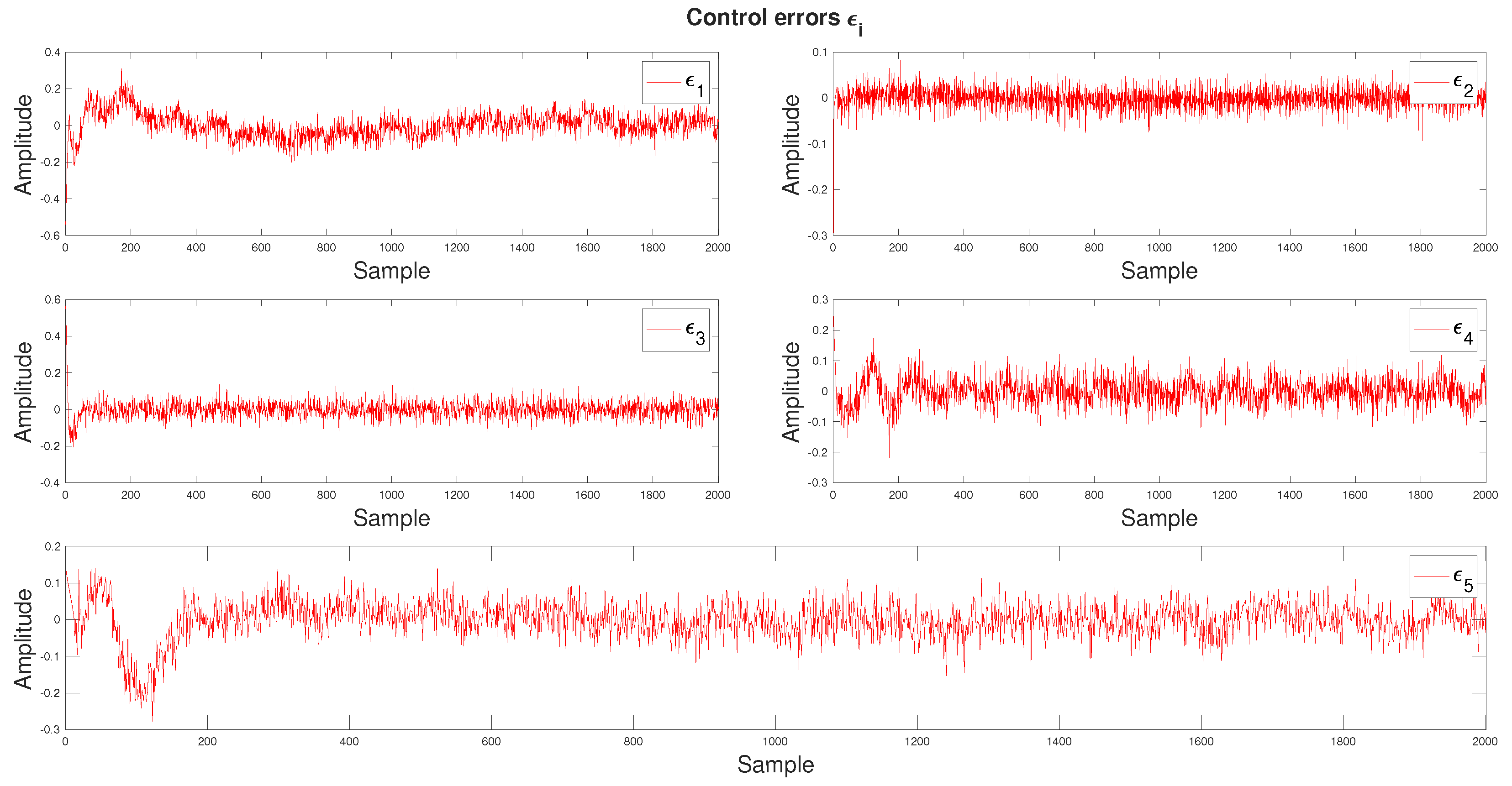
Figure 3 presents the simulation data generated with Gaussian noise. The noise parameters for each ${\sigma }_i$ variable were randomly selected.

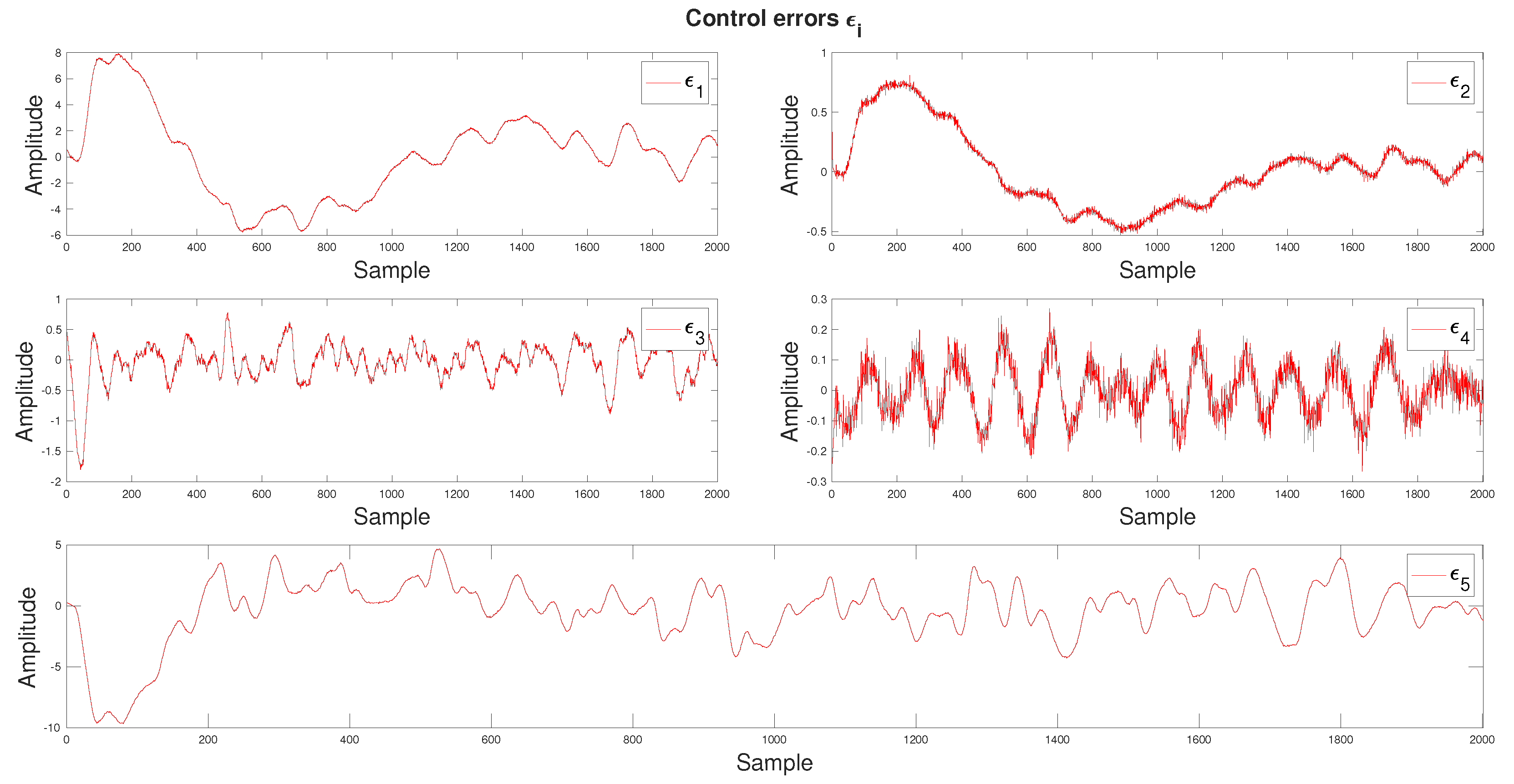
For the second scenario, both Gaussian and Cauchy disturbances were randomly chosen and a sinusoidal signal with a frequency of 30 Hz was added. The trends resulting from these assumptions are illustrated in Figure 4.

Because the relationships between the regulation errors from the control loop are known, Figure 5 shows the expected causality diagram for the simulation model. The solid line indicates a direct relationship and the dashed line indicates an indirect relationship.

4. Analysis of Simulation Results

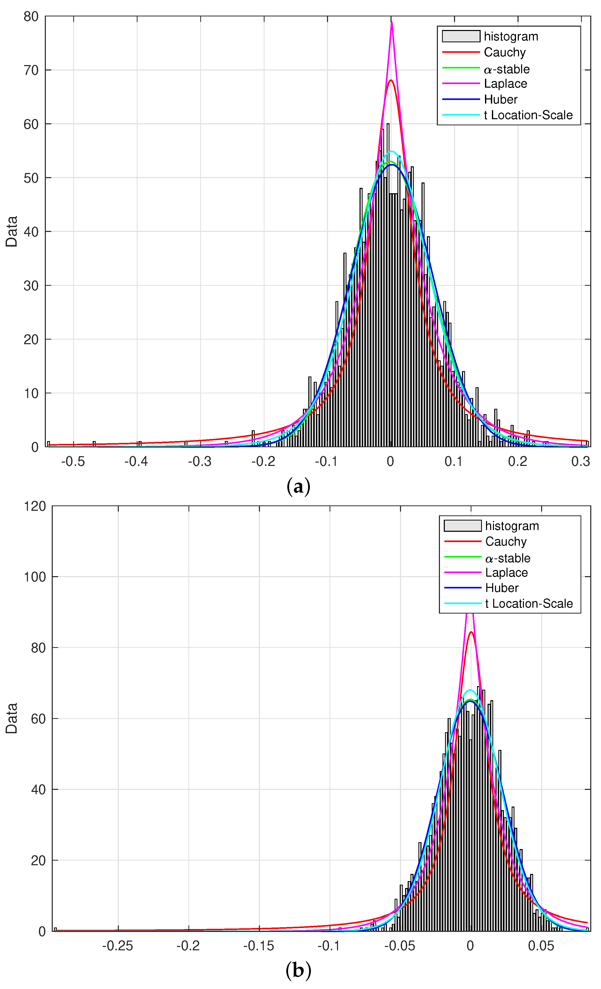
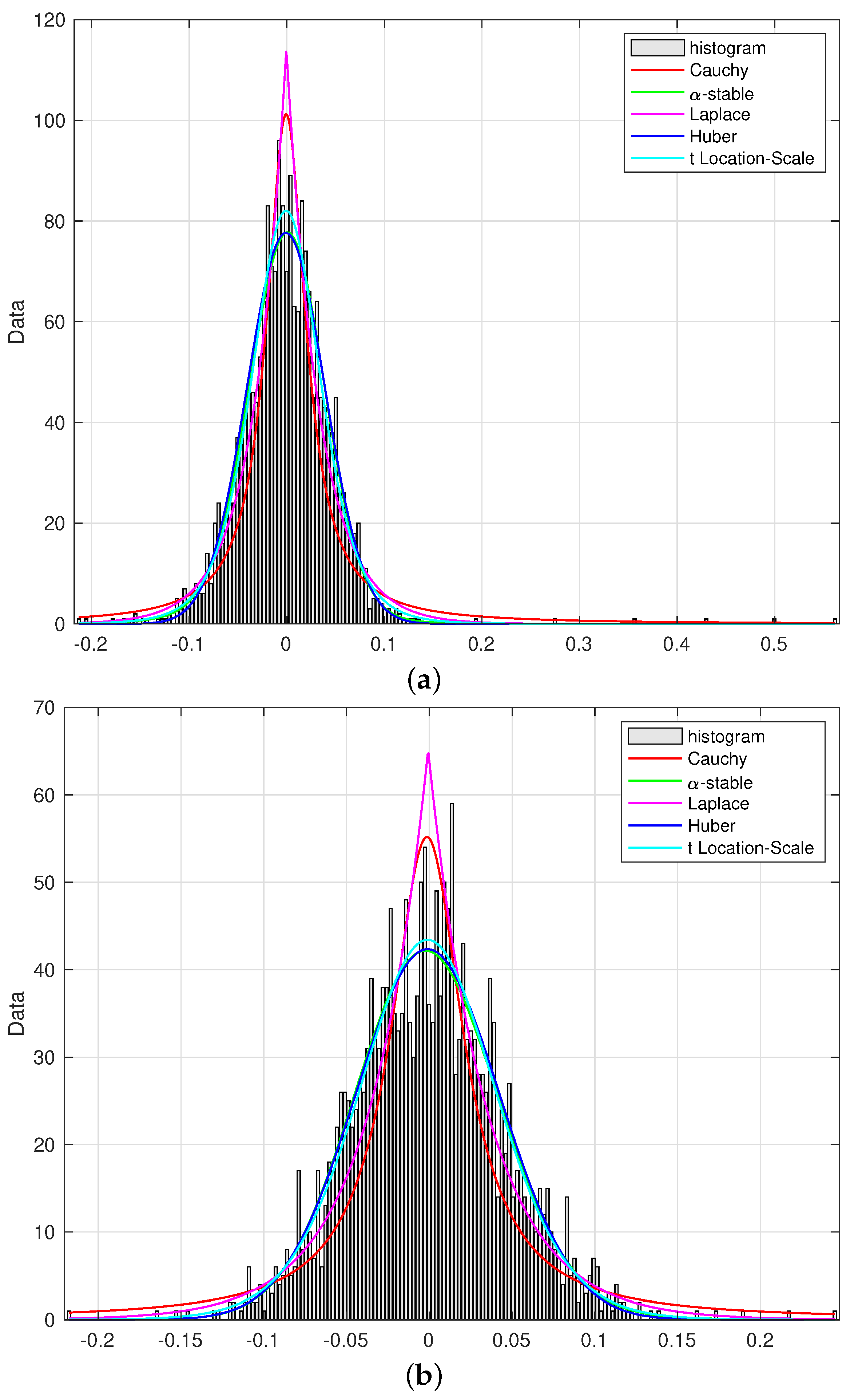
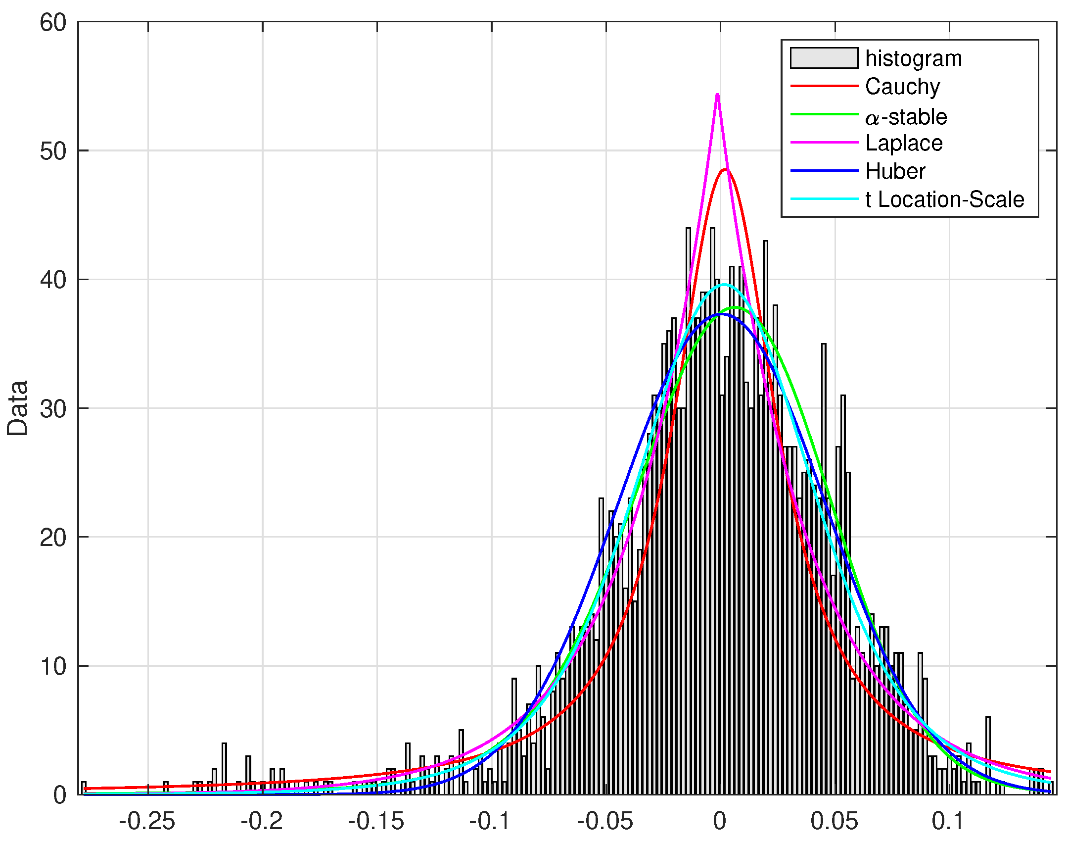
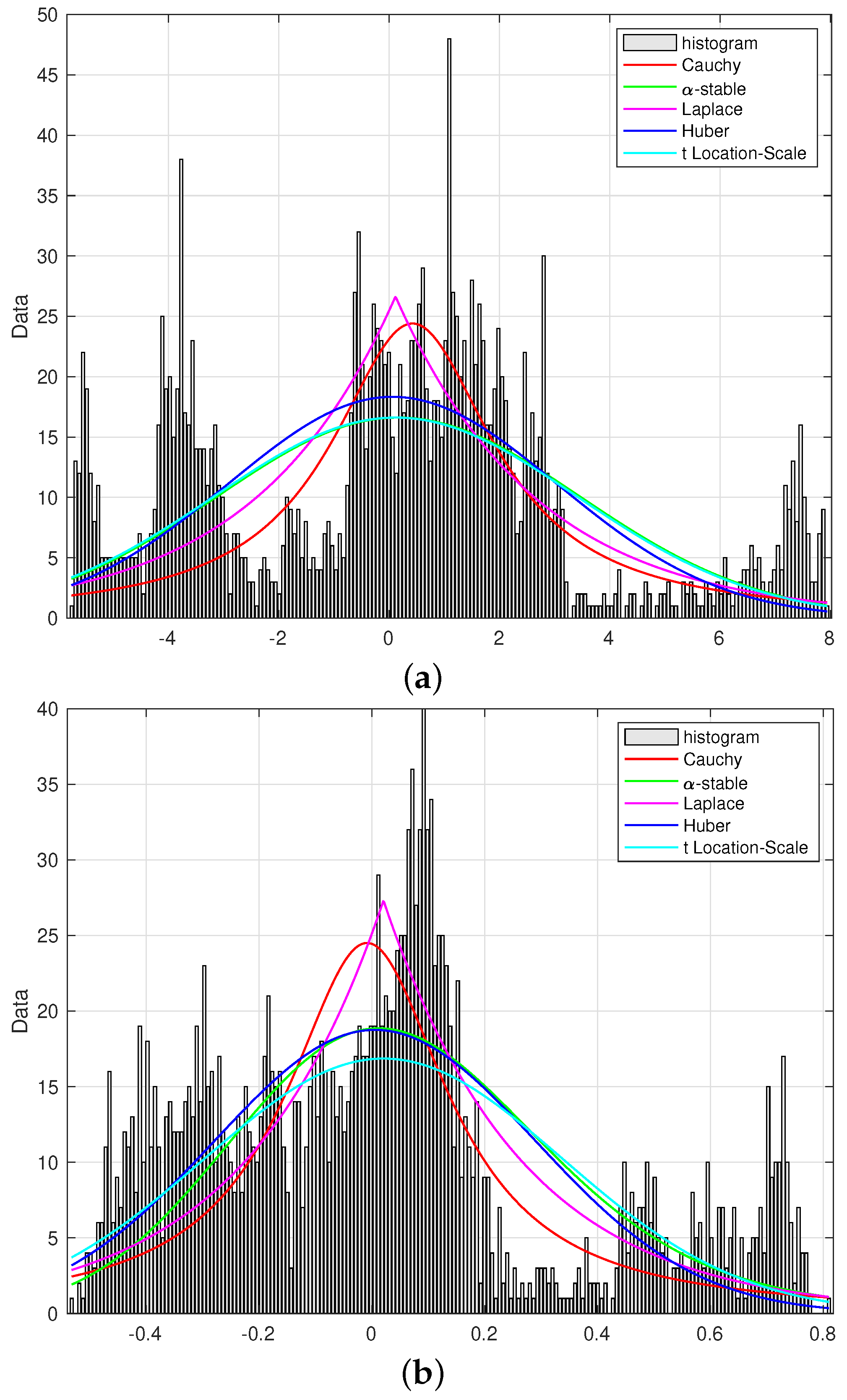
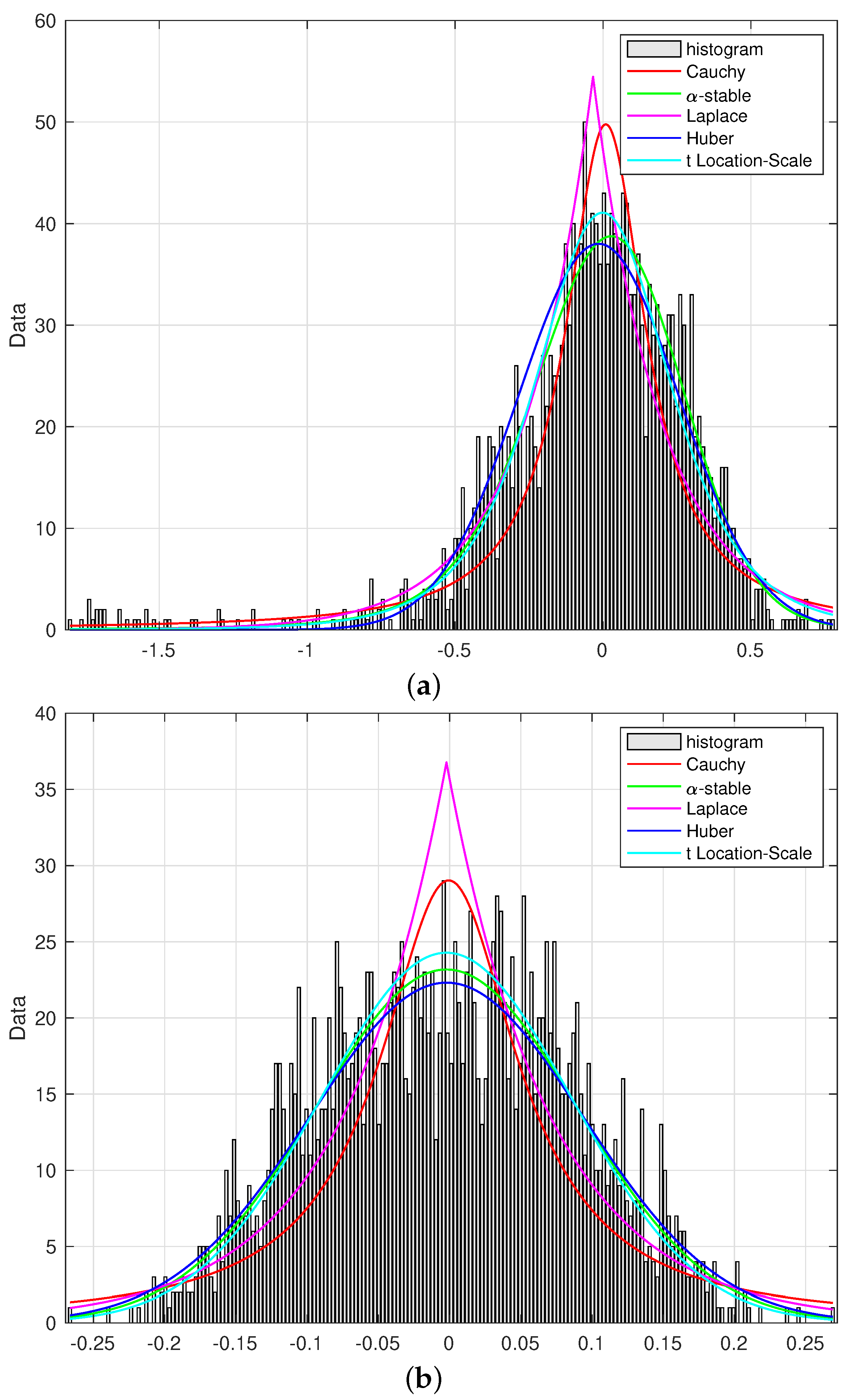
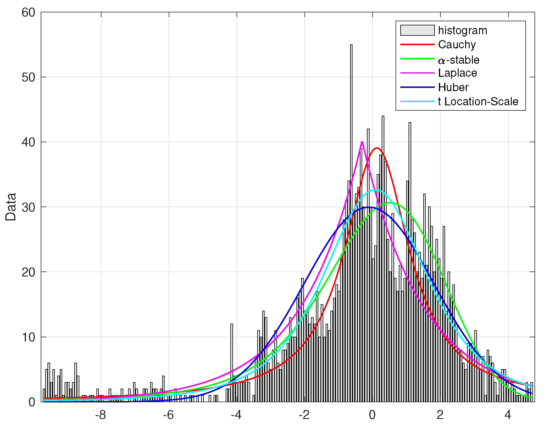
Analysis using the Transfer Entropy approach begins with the determination of probability distributions adjusted separately for each regulation error. This applies to data generated with Gaussian noise as well as to data with both Gaussian noise and Cauchy disturbance. The results for Cauchy, $\alpha$-stable, Laplace, Huber, and t-location scale distribution fitting are presented in Figure 6, Figure 7 and Figure 8 and Figure 9, Figure 10 and Figure 11, respectively.

The data generated with Gaussian noise are fairly normal and close to a normal distribution. A visual evaluation shows that the fit of the probability distributions is satisfactory, especially for the $\alpha$-stable distribution.

In the second case, data are generated with both Gaussian noise and Cauchy disturbance, with an added sinusoidal signal of 30 Hz frequency. For the most part, these data do not exhibit sufficient normality to be regarded as having been drawn from a normal distribution. In particular, this applies to the regulation errors ${ϵ}_1$ and ${ϵ}_2$. In the first place, this indicates the presence of outliers. According to [36], an outlier is defined as ”an observation which deviates so much from other observations as to arouse suspicions that it was generated by a different mechanism.” The presence of outliers has a significant effect on data analysis, as they increase the variance of the signal, reduce the power of statistical tests during analysis [37], disturb the normality of the signal and introduce fat tails [38], and introduce bias in regression analyses [39]. Outliers can be caused by erroneous observations or inherent data variability. There are many approaches for detecting these phenomena and removing them from data, i.e., the Interquartile Range method (IQR) [40], generalized Extreme Studentized Deviate (ESD) [41], and Hampel filter [42]. However, the phenomenon observed in the histograms shown here is the result of loop oscillations, and can be omitted in this case.

Assessment of the fit quality of the probability distributions selected for analysis cannot consist of a solely visual evaluation. To objectively determine which PDF best fits the regulation error histogram, a fit indicator is used. The fitting indexes are calculated using the mean square error between the empirical histogram heights and the value of the fitted probabilistic density function as evaluated at the middle of the respective histogram bin. The results for the dataset with Gaussian noise are presented in

Table 2. Fit indicators for the dataset with Gaussian noise.

	Cauchy	$\mathit{\alpha }$-Stable	Laplace	Huber	t Location-Scale
${ϵ}_1$	3.3440	1.4925	2.4805	1.5098	1.5333
${ϵ}_2$	3.6252	1.3049	2.7709	1.3007	1.4069
${ϵ}_3$	3.3966	1.4344	2.2947	1.5182	1.5246
${ϵ}_4$	3.5771	1.9684	2.8030	1.9850	1.9877
${ϵ}_5$	3.1062	1.9417	2.5749	1.9473	1.8361

and those for the dataset with Gaussian noise and Cauchy disturbance in

Table 3. Fit indicators for the dataset with both Gaussian noise and Cauchy disturbance.

	Cauchy	$\mathit{\alpha }$-Stable	Laplace	Huber	t Location-Scale
${ϵ}_1$	5.1540	5.7679	5.5035	5.6962	5.7589
${ϵ}_2$	5.0164	5.0727	4.9170	4.9768	4.9432
${ϵ}_3$	3.1914	1.9279	2.9657	2.1143	2.1835
${ϵ}_4$	3.9075	2.2738	3.6509	2.3228	2.3033
${ϵ}_5$	3.5362	3.1455	3.8385	3.4425	3.1752

. The lowest values of the fit indicator (which is considered the best fitting) for each ${ϵ}_i$ are marked in blue and bold.

As shown in Table 2, for the dataset with Gaussian noise the $\alpha$-stable distribution appears to have the best fit in the case of regulation errors ${ϵ}_1$, ${ϵ}_3$, and ${ϵ}_4$. For the regulation error ${ϵ}_2$, it is Huber distribution, and for the ${ϵ}_5$ it is the t-location scale. In Table 3, the lowest value of the fit indicator is calculated for the $\alpha$-stable distribution for regulation errors ${ϵ}_3$, ${ϵ}_4$, and ${ϵ}_5$. The significantly different natures of the trends of the regulation errors ${ϵ}_1$ and ${ϵ}_2$ clearly affect the calculation of the fit indicators. In both cases, the value of the indicator is higher than that determined for the regulation errors ${ϵ}_3$, ${ϵ}_4$, and ${ϵ}_5$. Nonetheless, the best fit for ${ϵ}_1$ is characterized by the Cauchy distribution and for the ${ϵ}_2$ by the Laplace distribution.

The general conclusion for both datasets is that in most cases the $\alpha$-stable distribution has the best fit for each ${ϵ}_i$. Therefore, it is apparent that the determined TE coefficients are based on the $\alpha$-stable distribution with regard to the classical Transfer Entropy approach. The results for the dataset with Gaussian noise and for the dataset with both Gaussian noise and Cauchy disturbance are presented in Section 4.1 and Section 4.2, respectively.

4.1. Causality for the Dataset with Gaussian Noise

In this subsection, the simulation data impacted by the Gaussian noise is analyzed (see Figure 3). The relationships between five regulation errors of a simulation system are designated using the Transfer Entropy approach based on the Gaussian distribution and $\alpha$-stable distribution.

Results for simulation data impacted by Gaussian noise for the classic TE approach are impossible to present in the form of a table, as most values appear as $NaN$-type or $Inf$-type values. These are considered to be 0, which indicates no causality. There are two possible reasons for such poor behavior. The first is that the Gaussian distribution does not sufficiently fit the data. The second and more probable reason is that Gaussian disturbance is too weak, and does sufficiently not stimulate the simulation system.

When using the Transfer Entropy method based on the $\alpha$-stable distribution, the results turn out to be satisfactory. The TE coefficients are obtained, and are included in

Table 4. Calculated TE coefficients based on the $\alpha$-stable distribution for the dataset with Gaussian noise.

${\mathit{T}}_{\mathit{row}\to \mathit{column}}$	${\mathit{ϵ}}_1$	${\mathit{ϵ}}_2$	${\mathit{ϵ}}_3$	${\mathit{ϵ}}_4$	${\mathit{ϵ}}_5$
${ϵ}_1$	NA	0.1284	0.0729	0.0725	0.1016
${ϵ}_2$	0.1499	NA	0.0508	0.0387	0.0511
${ϵ}_3$	0.0450	0.0531	NA	0.0322	0.0401
${ϵ}_4$	0.0435	0.0371	0.0349	NA	0.0399
${ϵ}_5$	0.0430	0.0518	0.0409	0.0433	NA

. Because there is no objective method for applying a threshold value to the obtained entropy values, the highest entropy value in each row is marked in blue and bold. Although the above assumption forces us to show only the direct relationships, it is nonetheless possible to draw the causality graph, which is provided in Figure 12. The analysis of these results allows us to conclude that the change in the probability distribution has a positive effect on the quality of the Transfer Entropy method. Comparing the causality graph with the assumed one presented in Figure 5, it is inconsistent only in the case of the direction of the relationship between the regulation errors ${ϵ}_1$ and ${ϵ}_5$; in all other cases the causality is determined correctly.

4.2. Causality for the Dataset with Gaussian Noise and Cauchy Disturbance

In this subsection, the simulation data impacted by both Gaussian noise and Cauchy disturbance is analyzed (see Figure 4). Again, the Transfer Entropy approach based on the Gaussian probability distribution and $\alpha$-stable distribution is used on the simulation data.

The results for the first case are presented in

Table 5. Calculated TE coefficients based on Gaussian distribution for the dataset with both Gaussian noise and Cauchy disturbance.

${\mathit{T}}_{\mathit{row}\to \mathit{column}}$	${\mathit{ϵ}}_1$	${\mathit{ϵ}}_2$	${\mathit{ϵ}}_3$	${\mathit{ϵ}}_4$	${\mathit{ϵ}}_5$
${ϵ}_1$	$NA$	$\mathbf{0.1143}$	$0.0743$	$0.0608$	$0.0631$
${ϵ}_2$	$0.0589$	$NA$	$0.0556$	$0.0490$	$\mathbf{0.0653}$
${ϵ}_3$	$0.0568$	$0.0475$	$NA$	$0.0699$	$\mathbf{0.0854}$
${ϵ}_4$	$0.0285$	$0.0374$	$\mathbf{0.0547}$	$NA$	$0.0419$
${ϵ}_5$	$0.0685$	$0.0694$	$\mathbf{0.0886}$	$0.0646$	$NA$

. The causality graph relating to Table 5 is shown in Figure 13. The presented graph has little resemblance to the assumed one in Figure 5. The reason for such poor behavior may be a characteristic of the data. Continuous changes in the values of the regulation errors can be noticed, as well as a clear trend in the data. Previous research using real data [43] has shown that TE is not resistant to sudden changes in variables values; hence, the Transfer Entropy method proves to be ineffective, and the values determined through it for the coefficients should be disregarded entirely.

The results for the second case are presented in

Table 6. Calculated TE coefficients based on the $\alpha$-stable distribution for the dataset with both Gaussian noise and Cauchy disturbance.

${\mathit{T}}_{\mathit{row}\to \mathit{column}}$	${\mathit{ϵ}}_1$	${\mathit{ϵ}}_2$	${\mathit{ϵ}}_3$	${\mathit{ϵ}}_4$	${\mathit{ϵ}}_5$
${ϵ}_1$	$NA$	$\mathbf{0.1154}$	$0.0729$	$0.0599$	$0.0601$
${ϵ}_2$	$0.0561$	$NA$	$0.0540$	$0.0491$	$\mathbf{0.0666}$
${ϵ}_3$	$0.0568$	$0.0475$	$NA$	$0.0699$	$\mathbf{0.0854}$
${ϵ}_4$	$\mathbf{0.0772}$	$0.0284$	$0.0521$	$NA$	$0.0380$
${ϵ}_5$	$0.0643$	$0.0695$	$\mathbf{0.0888}$	$0.0623$	$NA$

. The causality graph relating to Table 6 is shown in Figure 14.

The resulting causality relationships are only partially correct. Precise indications refer to regulation errors ${ϵ}_4\to {ϵ}_1$ and ${ϵ}_2\to {ϵ}_5$. The other relationships resulting from the Transfer Entropy calculations are misleading, and do not reflect those presented in Figure 5 for the assumed causality graph. Many questions arise from these results; in particular, it seems that changing the probability density function from a Gaussian distribution to an $\alpha$-stable distribution is effective for a dataset containing Gaussian noise. Of course, we are dealing here with data of a different nature, for which the solution can only be a deeper data analysis [24].

5. Conclusions and Further Research

The presented considerations aim to improve the model-free Transfer Entropy method by altering a key element in the causality detection approach. The original method utilizes the Gaussian probability distribution function and considers the process data as it is. In this paper, we have hypothesized that the identification process depends on the PDF fitting; thus, we propose a modification using common PDFs such as the Cauchy, $\alpha$-stable, Laplace, Huber, and t-location scale distributions. It is challenging to compare the TE method with other approaches. Though minor modeling assumptions are made in estimating the transfer entropy in this paper, in general the TE approach itself does not require a model of the analyzed process, while other methods typically assume process models. However, process models are seldom known in the process industry, and any misfitting in modeling can lead to confusion about whether responsibility for any particular issue lies with the model or the approach used for causality detection. Therefore, methods requiring model assumptions are not considered here, as the modeling effort would lead to increased complexity without any positive trade-offs.

In this study, we have examined two variants of simulated data, the first including distortion by Gaussian noise and the second including distortion by both Gaussian noise and Cauchy disturbance. In addition, a sinusoidal signal was added to the Cauchy disturbance to simulate known frequency loop oscillations and their propagation. The time series data represent regulation errors (${ϵ}_1$, ${ϵ}_2$, ${ϵ}_3$, ${ϵ}_4$, and ${ϵ}_5$). Due to the high computational complexity of the TE approach, we used short datasets for analysis, with the main focus on using the modified Transfer Entropy algorithm with the collected data in order to generate causality graphs.

The complexity of causality analysis is highlighted in the paper, as there is no single solution that can be applied to every case. The study considers two simulation examples. The first example was analyzed using the TE approach based on the $\alpha$-stable distribution, and was found to workseffectively. We demonstrate that their proposed methodology for selecting the proper probability distribution is successful in this specific case. However, applying the same method to the second example does not provide clear interpretations; the results become ambiguous, variable, unrepeatable, and difficult to interpret. The inclusion of a sinusoidal signal in the system to simulate potential loop oscillations seems to pose a challenge to the studied approach. The reason for this is difficult to determine, and could be due to factors such as inaccurate PDF fitting (especially for regulation errors ${ϵ}_1$ and ${ϵ}_2$), strong signal amplitude changes, fat tails, or other unknown factors. This represents a significant challenge, as oscillations are common in industrial systems.

Research has confirmed that in the case of the Transfer Entropy approach it is not possible to analyze only one factor. There are many variables involved in proper analysis. Certainly, one should not only focus on the method itself and its properties, as it is especially important to evaluate the the data. One helpful solution is data decomposition, as it involves analysis of the signal components. The first step is to identify the different sources of noise and oscillations and to analyze the statistical properties of the residue. Various factors should be considered before selecting or adopting an appropriate methodology.

The preceding analysis serves as motivation for further investigations in this area. Addressing this research challenge requires a distinct approach, as simulations alone are insufficient. A comprehensive and comparative analysis should be performed on several industrial examples while taking into account the various complexities involved. Although this task may be more challenging and demanding, it provides an opportunity to gain deeper insights into the problem and, potentially leading to the discovery of a viable solution.

References

1. Rubin, D.B. Estimating causal effects of treatments in randomized and nonrandomized studies. J. Educ. Psychol. 1974, 66, 688–701. [Google Scholar] [CrossRef] [Green Version]
2. Reichenbach, H. The Direction of Time; University of Los Angeles Press: Berkeley, CA, USA, 1956. [Google Scholar]
3. Dehejia, R.H.; Wahba, S. Causal effects in nonexperimental studies: Reevaluating the evaluation of training programs. J. Amer. Statist. Assoc. 1999, 94, 1053–1062. [Google Scholar] [CrossRef]
4. Mani, S.; Cooper, G. Causal discovery from medical textual data. In Proceedings of the AMIA Symposium, Los Angeles, CA, USA, 4–8 November 2000; Volume 542. [Google Scholar]
5. Imbens, G.W. Nonparametric estimation of average treatment effects under exogeneity: A review. Rev. Econ. Stat. 2004, 86, 4–29. [Google Scholar] [CrossRef] [Green Version]
6. Hernan, M.A.; Robins, J.M. Causal Inference; CRC Press: Boca Raton, FL, USA, 2020. [Google Scholar]
7. Ebert-Uphoff, I.; Deng, Y. Causal discovery for climate research using graphical models. JCLI 2012, 25, 5648–5665. [Google Scholar] [CrossRef] [Green Version]
8. Li, J.; Zaiane, O.R.; Osornio-Vargas, A. Discovering statistically significant co-location rules in datasets with extended spatial objects. In Proceedings of the 16th International Conference, DaWaK 2014, Munich, Germany, 2–4 September 2014; pp. 124–135. [Google Scholar]
9. Amin, M.T. An integrated methodology for fault detection, root cause diagnosis, and propagation pathway analysis in chemical process systems. Clean. Eng. Technol. 2021, 4, 100187. [Google Scholar] [CrossRef]
10. Liu, J.; Lim, K.W.; Ho, W.K.; Tan, K.C.; Srinivasan, R.; Tay, A. The intelligent alarm management system. IEEE Softw. 2003, 20, 66–71. [Google Scholar]
11. Zheng, Y.; Fang, H.; Wang, H.O. Takagi-Sugeno fuzzy model-based fault detection for networked control systems with Markov delays. IEEE Trans. Syst. Man Cybern. B 2006, 36, 924–929. [Google Scholar]
12. Yin, S.; Ding, S.; Haghani, A.; Hao, H.; Zhang, P. A comparison study of basic data-driven fault diagnosis and process monitoring methods on the benchmark Tennessee Eastman process. J. Process Control. 2012, 22, 1567–1581. [Google Scholar] [CrossRef]
13. Zhong, M.; Ding, S.X.; Ding, E.L. Optimal fault detection for linear discrete time-varying systems. Automatica 2010, 46, 1395–1400. [Google Scholar]
14. Ding, S.; Zhang, P.; Yin, S.; Ding, E. An integrated design framework of fault tolerant wireless networked control systems for industrial automatic control applications. IEEE Trans. Ind. Inform. 2013, 9, 462–471. [Google Scholar] [CrossRef]
15. Gokas, F. Distributed Control of Systems over Communication Networks. Ph.D. Thesis, University of Pennsylvania, Philadelphia, PA, USA, 2000. [Google Scholar]
16. Wiener, N. The Theory of Prediction; Modern Mathematics for Engineers; Beckenbach, E.F., Ed.; McGraw-Hill: New York, NY, USA, 1956; Volume 8, pp. 3269–3274. [Google Scholar]
17. Duan, P.; Yang, F.; Chen, T.; Shah, S.L. Detection of direct causality based on process data. In Proceedings of the 2012 American Control Conference (ACC), Montreal, QC, Canada, 27–29 June 2012; pp. 3522–3527. [Google Scholar] [CrossRef]
18. Duan, P. Information Theory-Based Approaches for Causality Analysis with Industrial Applications. Ph.D. Thesis, University of Alberta, Edmonton, AB, Canada, 2014. [Google Scholar]
19. Lee, J.; Nemati, S.; Silva, I.; Edwards, B.A.; Butler, J.P.; Malhotra, A. Transfer entropy estimation and directional coupling change detection in biomedical time series. BioMed. Eng. Online 2012, 11, 1315–1321. [Google Scholar] [CrossRef] [PubMed] [Green Version]
20. Kraskov, A.; Stögbauer, H.; Grassberger, P. Estimating mutual information. Phys. Rev. E 2004, 69, 066138. [Google Scholar] [CrossRef] [PubMed] [Green Version]
21. Bossomaier, T.; Barnett, L.; Harré, M.; Lizier, J. An Introduction to Transfer Entropy; Springer: Cham, Switzerland, 2016. [Google Scholar] [CrossRef]
22. Lizier, J.T. JIDT: An Information-Theoretic Toolkit for Studying the Dynamics of Complex Systems. Front. Robot. AI 2014, 1, 11. [Google Scholar] [CrossRef] [Green Version]
23. Wollstadt, P.; Lizier, J.; Vicente, R.; Finn, C.; Martínez Zarzuela, M.; Mediano, P.; Novelli, L.; Wibral, M. IDTxl: The Information Dynamics Toolkit xl: A Python package for the efficient analysis of multivariate information dynamics in networks. J. Open Source Softw. 2019, 4, 1081. [Google Scholar] [CrossRef]
24. Falkowski, M.J. Causality analysis incorporating outliers information. In Outliers in Control Engineering. Fractional Calculus Perspective; De Gruyter: Berlin, Germany; Boston, MA, USA, 2022; pp. 133–148. [Google Scholar] [CrossRef]
25. Falkowski, M.J.; Domański, P.D.; Pawłuszewicz, E. Causality in Control Systems Based on Data-Driven Oscillation Identification. Appl. Sci. 2022, 12, 3784. [Google Scholar] [CrossRef]
26. Jafari-Mamaghani, M.; Tyrcha, J. Transfer Entropy Expressions for a Class of Non-Gaussian Distributions. Entropy 2014, 16, 1743. [Google Scholar] [CrossRef] [Green Version]
27. Schreiber, T. Measuring information transfer. Phys. Rev. Lett. 2000, 85, 461–464. [Google Scholar]
28. Yang, F.; Xiao, D. Progress in Root Cause and Fault Propagation Analysis of Large-Scale Industrial Processes. J. Control. Sci. Eng. 2012, 2012, 478373. [Google Scholar]
29. Vincente, R.; Wibral, M.; Lindner, M.; Pipa, G. Transfer entropy—A model-free measure of effective connectivity for the neurosciences. J. Comput. Neurosci. 2011, 30, 45–67. [Google Scholar] [CrossRef] [Green Version]
30. Kayser, A.S.; Sun, F.; Desposito, M. A comparison of Granger causality and coherency in fMRI-based analysis of the motor system. Hum. Brain Mapp. 2009, 30, 3475–3494. [Google Scholar] [CrossRef] [Green Version]
31. Domański, P.D. Study on Statistical Outlier Detection and Labelling. Int. J. Autom. Comput. 2020, 17, 788–811. [Google Scholar] [CrossRef]
32. Croux, C.; Dehon, C. Robust Estimation of Location and Scale; Wiley: Hoboken, NJ, USA, 2014. [Google Scholar]
33. Domański, P.D. Non-Gaussian Statistical Measures of Control Performance. Control Cybern. 2017, 46, 259–290. [Google Scholar]
34. Domański, P.D. Non-Gaussian properties of the real industrial control error in SISO loops. In Proceedings of the 19th International Conference on System Theory, Control and Computing, Sinaia, Romania, 19–21 October 2015; pp. 877–882. [Google Scholar]
35. Domanski, P. Control Performance Assessment: Theoretical Analyses and Industrial Practice; Springer International Publishing: Cham, Switzerland, 2020. [Google Scholar]
36. Hawkins, D.M. Identification of Outliers; Chapman and Hall: London, UK; New York, NY, USA, 1980. [Google Scholar]
37. Osborne, J.W.; Overbay, A. The power of outliers (and why researchers should ALWAYS check for them), Practical Assessment. Res. Eval. 2004, 9, 1–8. [Google Scholar]
38. Taleb, N. Statistical Consequences of Fat Tails: Real World Preasymptotics, Epistemology, and Applications. arXiv 2020, arXiv:2001.10488. [Google Scholar]
39. Rousseeuw, P.J.; Leroy, A.M. Robust Regression and Outlier Detection; John Wiley & Sons, Inc.: New York, NY, USA, 1987. [Google Scholar]
40. Whaley, D.L. The Interquartile Range: Theory and Estimation. Master’s Thesis, East Tennessee State University, Johnson City, TN, USA, 2005. [Google Scholar]
41. Rosner, B. Percentage points for a generalized esd many-outlier procedure. Technometrics 1983, 25, 165–172. [Google Scholar] [CrossRef]
42. Pearson, R.K. Mining Imperfect Data: Dealing with Contamination and Incomplete Records; SIAM: Philadelphia, PA, USA, 2005. [Google Scholar]
43. Falkowski, M.J.; Domański, P.D. Impact of outliers on determining relationships between variables in large-scale industrial processes using Transfer Entropy. In Proceedings of the 2020 7th International Conference on Control, Decision and Information Technologies (CoDIT), Prague, Czech Republic, 29 June–2 July 2020; Volume 1, pp. 807–812. [Google Scholar] [CrossRef]
Figure 1. Simulated multi-loop PID-based control layout.
Applsci 13 05849 g001
Figure 2. The industrial implementation of feedforward disturbance decoupling.
Applsci 13 05849 g002
Figure 3. Control error time series for the simulation data with Gaussian noise.
Applsci 13 05849 g003
Figure 4. Control error time series for the data with Gaussian noise and Cauchy disturbance.
Applsci 13 05849 g004
Figure 5. The causality diagram of the considered simulated benchmark example.
Applsci 13 05849 g005
Figure 6. Histograms with PDF fitting for dataset with Gaussian noise: (a) control error ϵ 1 and (b) control error ϵ 2 .
Applsci 13 05849 g006
Figure 7. Histograms with PDF fitting for dataset with Gaussian noise: (a) control error ϵ 3 and (b) control error ϵ 4 .
Applsci 13 05849 g007
Figure 8. Histograms with PDF fitting for dataset with Gaussian noise (control error ϵ 5 ).
Applsci 13 05849 g008
Figure 9. Histograms with PDF fitting for dataset with Gaussian noise and Cauchy disturbance: (a) control error ϵ 1 and (b) control error ϵ 2 .
Applsci 13 05849 g009
Figure 10. Histograms with PDF fitting for dataset with Gaussian noise and Cauchy disturbance: (a) control error ϵ 3 and (b) control error ϵ 4 .
Applsci 13 05849 g010
Figure 11. Histograms with PDF fitting for dataset with Gaussian noise and Cauchy disturbance (control error ϵ 5 ).
Applsci 13 05849 g011
Figure 12. Causality diagram for the dataset with Gaussian noise using the TE approach based on the α -stable distribution.
Applsci 13 05849 g012
Figure 13. Causality diagram for the dataset with both Gaussian noise and Cauchy disturbance using the Transfer Entropy approach based on the Gaussian distribution.
Applsci 13 05849 g013
Figure 14. Causality diagram for the dataset with both Gaussian noise and Cauchy disturbance using the Transfer Entropy approach based on the α -stable distribution.
Applsci 13 05849 g014