Article

A New Insight into Reliability Data Modeling with an Exponentiated Composite Exponential-Pareto Model

by
Bowen Liu
†,‡ and
Malwane M. A. Ananda
*,†,‡
Department of Mathematical Sciences, University of Nevada, Las Vegas, NV 89154, USA
*
Author to whom correspondence should be addressed.
Current address: 4505 S Maryland Pkwy, Las Vegas, NV 89154, USA.
These authors contributed equally to this work.
Appl. Sci. 2023, 13(1), 645; https://doi.org/10.3390/app13010645
Submission received: 14 November 2022 / Revised: 23 December 2022 / Accepted: 30 December 2022 / Published: 3 January 2023
(This article belongs to the Special Issue Reliability Techniques in Engineering Projects)

Abstract

:
It is observed that, for some of the data in engineering and medical fields, the hazard rates increase to a high peak at the beginning and quickly decrease to a low level. In the context of survival analysis, such a hazard rate is called a upside-down bathtub hazard rate. In this paper, we investigated the properties of a model named exponentiated exponential-Pareto distribution. The model was recently proposed and applied to insurance data. We demonstrated that the model has upside-down bathtub-shaped hazard rates with specific choices of parameters. The theoretical properties such as moments, survival functions, and hazard functions were derived. The parameter estimation procedures were also introduced. We then briefly discussed the goodness-of-fit tests of the model with the simulations. Finally, we applied the model to a specific time-to-event data set along with a comparison of the performances with previous existing models. When compared to previous proposed models, the exponentiated exponential-Pareto model demonstrated good performance when fitting to such data sets.

1. Introduction

Reliability data modeling has been an important topic in many different fields such as engineering, biology, and medical sciences. For data sets collected in real life, the hazard rates can show different shapes: monotone increasing, monotone decreasing, bathtub-shaped and upside-down bathtub (UBT)-shaped. While the data sets with monotone or bathtub hazard rates were deeply investigated with different types of parametric models, the data sets with UBT shapes were not as well explored as the others.
In fact, data with UBT-shaped hazard rates appeared frequently in the existing literature. For instance, for the Veteran’s Administration lung cancer trial data [1,2,3], the mortality rate was very low at the beginning, quickly rose to a high peak, and then slowly decreased. This suggests that the data are associated with a UBT-shaped hazard rate. This was also observed in several other data sets from medical and engineering fields [4,5,6].
To model data with UBT-shaped hazard rates, many parametric models have been proposed in the past. For example, the transmuted Rayleigh distribution [6] was proposed and demonstrated good performance when fitted to a reliability data set with UBT-shaped hazard rates. For more models proposed for this type of data, readers are referred to [7,8,9,10,11,12].
The concept of the generalized composite distributions was recently proposed to provide better options for fitting right skewed data with a high peak. It was demonstrated that special members from this family, such as exponentiated exponential-Pareto (EEP) distribution and exponentiated inverse-gamma Pareto (EIGP) distribution, can provide satisfactory performances to multiple insurance data sets [13,14]. Moreover, these data sets have very similar features to the ones with UBT-shaped hazard rates. Thus, utilizing these distributions to fit the data sets with UBT-shaped hazard rates seems to be appropriate.
The rest of the paper is organized as follows. Section 2 introduces the concept of the composite distribution. Section 2.2 provides the concept and some properties of the generalized exponentiated composite distribution (GEC). In Section 3, a special model named exponentiated exponential-Pareto (EEP) model is discussed. The parameter estimation of the EEP distribution is introduced in Section 4. In Section 5, by utilizing the goodness-of-fit (GoF) test, a limited simulation study is given to demonstrate the performance of the model associated with the exponent parameter. A real data analysis is presented in Section 6. Finally, the concluding remark and future directions are provided in Section 7.

2. Related Work

We start by introducing the concepts of composite distributions and generalized exponentiated composite distributions.

2.1. The Composite Distributions

Let Y be a random variable that only takes non-negative real numbers. Let f Y ( y ) be the probability density function (pdf) of Y. The formal definition of a composite pdf f Y ( y ) is given as follows [15]:
f Y ( y ; α 1 , α 2 , θ ) = c f 1 ( y ; α 1 , θ ) 0 y < θ c f 2 ( y ; α 2 , θ ) y θ ,
where c stands for the normalizing constant, θ is the parameter that denotes the location of probability density change, f 1 is the pdf of Y when Y is between 0 and θ , and α 1 represents the parameters of f 1 ; f 2 is the pdf of Y when Y is greater than θ , and α 2 represents the parameters of f 2 . It is assumed that both f 1 and f 2 are smooth functions on their supports. f 1 is generally called the head pdf of f Y , while f 2 is referred to as the tail pdf of f Y .
In real practice, f Y ( y | α 1 , α 2 , θ ) is usually assumed to be continuous and differentiable. Thus, the following conditions are imposed:
lim y θ f Y ( y ; α 1 , α 2 , θ ) = lim y θ + f Y ( y ; α 1 , α 2 , θ ) lim y θ d f Y ( y ; α 1 , α 2 , θ ) d y = lim y θ + d f Y ( y ; α 1 , α 2 , θ ) d y .
In real practice, the Pareto distribution and the generalized Pareto distribution (GPD) are commonly used for modeling highly right-skewed data at the right tail due the theoretical properties of such distributions. However, both of these distributions can only fit the data beyond a specific threshold. Hence, they cannot be used to globally fit the data.
Many composite models with Pareto or GPD tails have been developed by utilizing the idea of composite distributions, including lognormal-GPD [15], lognormal-Pareto [16], exponential-Pareto [17,18], Weibull–Pareto [19,20,21], inverse gamma-Pareto [22], and so on. Moreover, Grün and Miljkovic [23] explored a large number of composite distributions with Pareto and GPD tails with a general framework of computational tools.
Composite models with a Pareto tail have been widely used in different fields such as actuarial data and reliability data modeling. While these models were frequently used in the literature, it was found that some of the models such as exponential-Pareto [24] and inverse gamma-Pareto [22] do not perform well when fitting real sets with right skewed distributions. Therefore, a new concept named generalized family of exponentiated composite distribution (GEC) was proposed to address the issue [14].
In the next subsection, we introduce the concept of generalized family of exponentiated composite distributions and the properties of this family.

2.2. A Generalized Family of Exponentiated Composite Distributions

A power transformation T = Y 1 η ( η > 0 ) on the original composite random variable Y generates an exponentiated composite random variable T with an exponentiated composite pdf. Correspondingly, T is denoted as the exponentiated composite random variable induced by the parent composite random variable Y [14]. The pdf of T can be expressed as follows:
f T ( t ; α 1 , α 2 , θ , η ) = c f 1 ( t η ; α 1 , θ ) η t η 1 0 t < θ 1 η c f 2 ( t η ; α 2 , θ ) η t η 1 t θ 1 η .
The pdf f T ( t ) is then referred as the exponentiated composite pdf induced by the parent composite pdf f Y ( y ) .
Subsequently, we derive the properties of the exponentiated composite random variable T induced by the parent composite random variable Y.

2.2.1. Moments

Suppose that a composite random variable Y has finite k-th moment μ k . The k-th moment of an exponentiated composite random variable T induced by Y was derived previously by Liu and Ananda [14] as follows:
E ( T k ) = E ( Y k η ) = μ k 1 η

2.2.2. Survival Function

Assume that Y is a composite random variable with the CDF F Y ( y ) , where F Y ( y ) = P ( Y y ) . The CDF of the corresponding exponentiated composite random variable T = Y 1 η can be represented:
F T ( t ) = P ( T t ) = P ( Y 1 η t ) = P ( Y t η ) = F Y ( t η ) .
The survival function of Y can then be represented as follows:
S T ( t ) = 1 F T ( t ) = 1 F Y ( t η ) .
Now, consider the pdf defined in Equation (1). Let F 1 ( y ; α 1 , θ ) and F 2 ( y ; α 2 , θ ) be the corresponding CDF of f 1 ( y ; α 1 , θ ) and f 2 ( y ; α 2 , θ ) . The CDF of a composite random variable Y can be expressed as follows:
F Y ( y ; α 1 , α 2 , θ ) = 0 y f Y ( t ; α 1 , α 2 , θ ) d t = c 0 y f 1 ( t ; α 1 , θ ) d t if y [ 0 , θ ) c [ 0 θ f 1 ( t ; α 1 , θ ) d t + θ y f 2 ( t ; α 2 , θ ) d t ] if y [ θ , ) = c F 1 ( y ; α 1 , θ ) if y [ 0 , θ ) c [ F 1 ( θ ; α 1 , θ ) + F 2 ( y ; α 2 , θ ) F 2 ( θ ; α 1 , θ ) ] if y [ θ , ) .
Correspondingly, the exponentiated composite random variable T induced by Y has a CDF as follows:
F T ( t ; α 1 , α 2 , θ ) = c F 1 ( t η ; α 1 , θ ) if t [ 0 , θ 1 η ) c [ F 1 ( θ ; α 1 , θ ) + F 2 ( t η ; α 2 , θ ) F 2 ( θ ; α 1 , θ ) ] if t [ θ 1 η , ) .
The corresponding survival function of T can then be expressed as follows:
S T ( t ; α 1 , α 2 , θ ) = 1 c F 1 ( t η ; α 1 , θ ) if t [ 0 , θ 1 η ) 1 c [ F 1 ( θ ; α 1 , θ ) + F 2 ( t η ; α 2 , θ ) F 2 ( θ ; α 1 , θ ) ] if t [ θ 1 η , ) .

2.2.3. Hazard Function

The hazard function of a random variable T is defined as follows:
h T ( t ) = lim Δ t S T ( t + Δ t ) S T ( t ) Δ t · S T ( t ) .
Given the assumption that T is an exponentiated composite random variable induced by the composite random variable Y, the hazard function of T can be represented as follows, with the pdf and CDF of its parent composite random variable Y:
h T ( t ) = f T ( t ) S T ( t ) = f Y ( t η ) η t η 1 1 F Y ( t η ) . = c f 1 ( t η ; α 1 , θ ) η t η 1 1 c F 1 ( t η ; α 1 , θ ) if t [ 0 , θ 1 η ) c f 2 ( t η ; α 2 , θ ) η t η 1 1 c [ F 1 ( θ ; α 1 , θ ) + F 2 ( t η ; α 2 , θ ) F 2 ( θ ; α 1 , θ ) ] if t [ θ 1 η , ) .

2.2.4. Quantile Function

The quantile function of a random variable Y is defined as follows:
Q Y ( p ) = inf { y R : p F Y ( y ) } ,
where p ( 0 , 1 ) .
Thus, if Y is a composite random variable and T is the exponentiated composite random variable induced by Y, then the quantile function of T can be represented as follows:
Q T ( p ) = inf { t R : p F T ( t ) } = inf { t R : p F Y ( t η ) } .
If F Y ( y ) is strictly increasing and continuous, the quantile function Q Y ( p ) is then the inverse function of F Y ( y ) :
Q Y ( p ) = F Y 1 ( p ) = { y R : F Y ( y ) = p } .
Correspondingly, the quantile function of T can be written as follows in terms of the pdf of its parent composite random variable Y:
Q T ( p ) = F T 1 ( p ) = { t R : F T ( t ) = p } = { t R : F Y ( t η ) = p } .

3. Special Model: Exponentiated Exponential-Pareto Distribution (EEP)

The exponential-Pareto (EP) composite distribution was first proposed by Teodorescu and Vernic in 2006 [17]. Suppose that Y is a EP random variable. Then, the pdf of Y is first defined as follows:
f Y ( y ; λ , θ ) = c λ e λ y 0 y < θ c α θ α y α + 1 y θ ,
Assuming that the continuity and differentiability conditions hold, we have the following:
lim y θ f Y ( y ; λ , θ ) = lim y θ + f Y ( y ; α 1 , α 2 , θ ) lim y θ d f Y ( y ; λ , θ ) d y = lim y θ + d f Y ( y ; λ , θ ) d y .
This generates a system of equations in terms of θ , α , and λ :
λ e λ θ = α θ 1 λ 2 e λ θ = α ( α + 1 ) θ 2 .
By simple calculation, λ can be expressed in terms of α and θ , as follows:
λ = α + 1 θ .
Additionally, by utilizing the system of equations, the value of α can be determined as the solution of the following equation:
( α + 1 ) e ( α + 1 ) = α .
Since the shape parameter α of a Pareto distribution is restricted to being positive, the above equation gives a unique solution:
α = 0.349976 .
Since we assume that f Y ( y ; λ , θ ) is a valid pdf, we can also obtain the unique solution for the normalizing constant c as follows:
c = 1 2 e ( α + 1 ) = 0.574464 .
Thus, the pdf of Y with one parameter θ can be written as follows:
f Y ( y ; θ ) = c ( α + 1 θ ) e ( α + 1 ) y θ y < θ c α θ α y α + 1 y θ ,
where c = 0.574464 , α = 0.349976 .
With the power transformation T = Y 1 η , T is obtained as an exponentiated exponential-Pareto (EEP) composite random variable. The pdf of T can be expressed as follows:
f T ( t ; θ , η ) = c ( α + 1 θ ) e ( α + 1 ) t η θ η t η 1 0 < t < θ 1 η c α θ α ( t η ) α + 1 η t η 1 t θ 1 η ,
Figure 1 shows the pdf of EEP distributions with different parameters. Notice that, when η > 1 , the pdf of EEP distribution is hump-shaped; we discuss this in detail in the next subsection.

3.1. Mode

Since both exponential distribution and Pareto distribution are associated with monotonically decreasing pdf, the pdf of the original EP distribution is also monotonically decreasing. Thus, as an composite distribution, EP still does not have the ability to model the data with hump-shaped frequency distributions. One of the advantages of the EEP distribution against the original EP distribution is that the EEP can have a pdf with a hump shape, or equivalently, the EEP distribution has a mode under certain conditions. We explore the conditions for such hump-shaped distributions in the following part:
Proposition 1.
Suppose that T is an EEP composite random variable. Assume that f T ( t ; θ , η ) is the pdf associated with T. Then, the mode of T exists if and only if η > 1 . When η > 1 , the mode of T is [ θ ( η 1 ) η ( α + 1 ) ] 1 η .
Proof of Proposition 1. 
First, suppose t θ 1 η ; then, f T ( t ; θ , η ) = c α θ α ( t η ) α + 1 η t η 1 .
Correspondingly, d f T ( t ; θ , η ) d t = ( α η 1 ) c α θ α η t α η 2 < 0 for all t θ 1 η .
Therefore, when t θ 1 η , f T ( t ; θ , η ) is monotonically decreasing.
Since f T ( t ; θ , η ) is continuous, this implies that the maximum of f T ( t ; θ , η ) must occur when t < θ 1 η if the maximum exists.
Assume t < θ 1 η , then f T ( t ; θ , η ) = c ( α + 1 θ ) e ( α + 1 ) t η θ η t η 1 .
When f T ( t ; θ , η ) is a positive real-valued function, maximizing f T ( t ; θ , η ) is equivalent to maximizing ln f T ( t ; θ , η ) . Thus, we use ln f T ( t ; θ , η ) for the rest of the derivations.
Then, ln f T ( t ; θ , η ) = ln ( c ) + ln ( α + 1 θ ) ( α + 1 ) t η θ + ln ( η ) + ( η 1 ) ln ( t ) .
Correspondingly, d ln f T ( t ; θ , η ) d t = ( α + 1 ) η t η 1 θ + η 1 t
Let d ln f T ( t ; θ , η ) d t = 0 . Then, we have the equation of t: η 1 = η ( α + 1 θ ) t η .
Notice that t > 0 . Hence, the above equation has a solution only when η > 1 . Therefore, the mode of T exists if and only if η > 1 .
When η 1 , the equation has a unique solution: t = [ θ ( η 1 ) η ( α + 1 ) ] 1 η . It can be shown that d 2 f T ( t ; θ , η ) d t 2 < 0 when t = [ θ ( η 1 ) η ( α + 1 ) ] 1 η . Thus, t = [ θ ( η 1 ) η ( α + 1 ) ] 1 η is the mode of T.
Therefore, the addition of the exponent parameter η in the EEP model definitely improves the flexibility of the original EP model since it can model the data with a hump-shaped distribution.

3.2. Moments

The k-th moments of the EEP distribution was derived by Liu and Ananda [13] as follows:
E ( T k ) = c ( θ α + 1 ) k η Γ ( k η + 1 ) Γ ( k η + 1 , α + 1 ) + c α θ k η α k η ,
where Γ ( α ) represents the Gamma function, namely Γ ( α ) = 0 u α 1 e u d u . Γ ( . , . ) When k η < α , the k-th moment is finite. Correspondingly, the mean of the EEP distribution is as follows:
E ( T ) = c ( θ α + 1 ) 1 η Γ ( 1 η + 1 ) Γ ( 1 η + 1 , α + 1 ) + c α θ 1 η α 1 η .
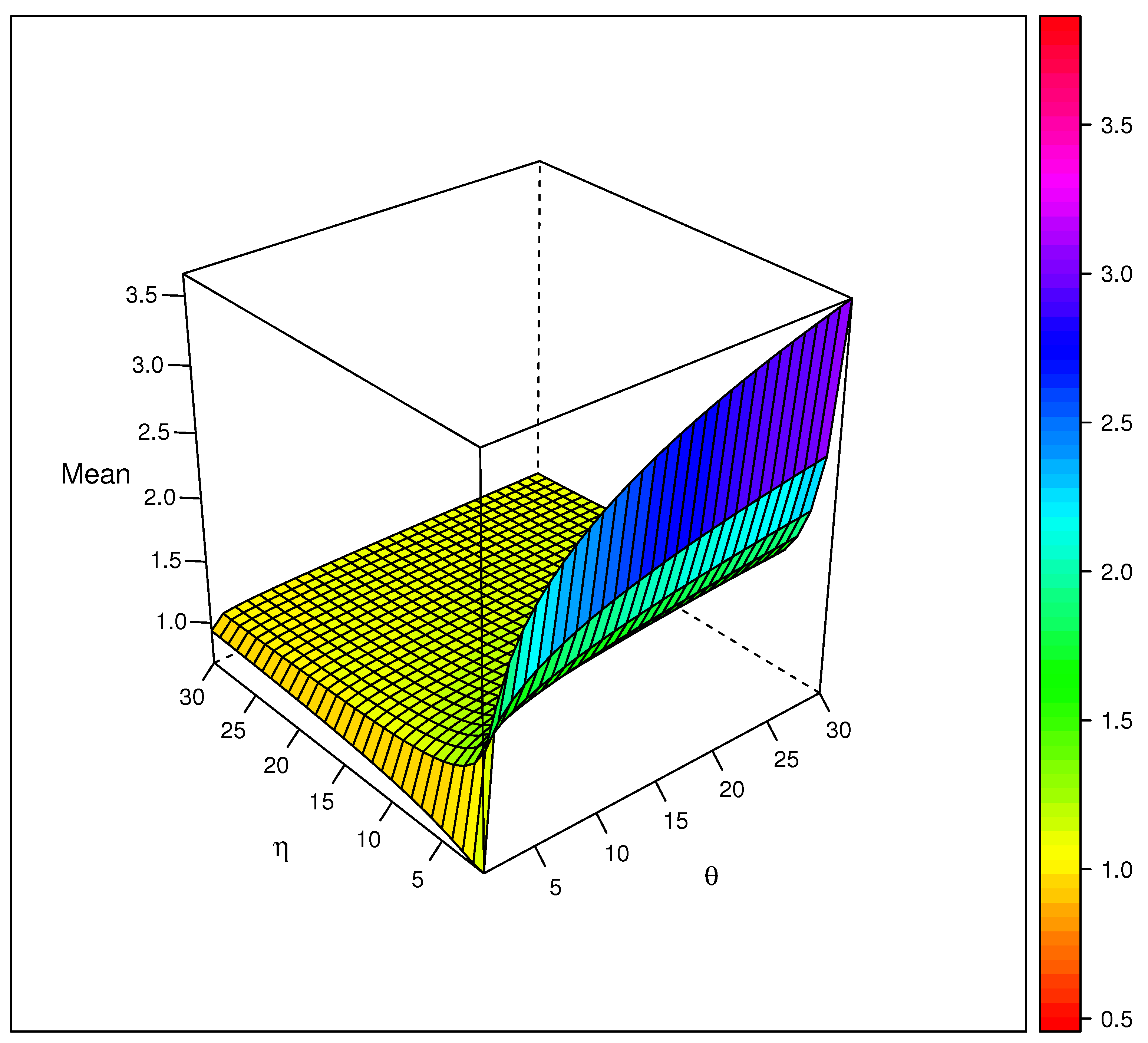
The mean of the EEP distribution is plotted in Figure 2. The figure shows that the mean is an increasing function of θ and a decreasing function of η for selected θ and η values.

3.3. Survival Function and Tail Properties

Since (11) is a continuous differentiable pdf, the cumulative distribution function (CDF) can be derived. By the definition of CDF, we have the following:
F T ( t ; θ , η ) = c 1 e ( α + 1 ) t η θ t < θ 1 η c 2 e ( α + 1 ) θ α t η α t θ 1 η .
Notice that the development of EP distribution guarantees that c ( 2 e ( α + 1 ) ) = 1 . Therefore,
F T ( t ; θ , η ) = c 1 e ( α + 1 ) t η θ t < θ 1 η 1 c θ α t η α t θ 1 η .
Since T is a continuous random variable, the survival function of T is provided correspondingly as follows:
S T ( t ; θ , η ) = 1 F T ( t ; θ , η ) ,
that is,
S T ( t ; θ , η ) = 1 c 1 e ( α + 1 ) t η θ t < θ 1 η c θ α t η α t θ 1 η .
Now, given that we derived the formula of CDF and the survival function of T, we can further discuss the tail properties of the EEP distribution.
Proposition 2.
If T follows an EEP distribution with a CDF F, then the distribution of T has a heavy tail.
Proof of Proposition 2. 
We only prove that lim t e λ t S T ( t ) = lim t c θ α e λ t t η α = for all λ > 0 .
Notice η α > 0 based on our assumption. Denote η α as the smallest integer greater than η α .
Then, since lim t c θ α e λ t = and lim t t η α = , apply L’Hospital rule η α times. We have lim t e λ t S T ( t ) = lim t c λ η α θ α e λ t i = 1 η α ( η α i ) t η α η α = .
Therefore, the distribution of T has a heavy tail.
Furthermore, we could also specify the conditions that an EEP distribution has a fat tail. Suppose that the survival function of a random variable X satisfies the following:
S ( x ) x β as x , α > 0
Notice that a distribution is said to have a fat tail when the tail index β < 2 . Notice that, for an EEP random variable T, S T ( t ) t η α . Therefore, only when η α < 2 , the EEP distribution is considered to have a fat tail.

3.4. Hazard Function

For a continuous random variable T, the hazard function is defined as follows:
h T ( t ) = f T ( t ) S T ( t ) .
Therefore, by utilizing the pdf and survival function of Y, the hazard function of a EEP random variable T can be derived as follows:
h T ( t ; θ , η ) = c ( α + 1 θ ) e ( α + 1 ) t η θ η t η 1 1 c + c e ( α + 1 ) t η θ t < θ 1 η α η t 1 t θ 1 η
Notice that h T ( t ; θ , η ) is monotonically decreasing when t θ 1 η . For some selections of θ and η values, the hazard function h T ( t : θ , η ) could be UBT. Figure 3 shows the hazard functions of EEP distributions with different parameters.

3.5. Quantile Function

The quantile function of a continuous random variable T is defined as the inverse function of its CDF F T . Since the explicit form of F T is derived in (10), we have the quantile function an EEP random variable T as follows:
F T 1 ( p ; θ , η ) = [ ln ( c c p ) θ α + 1 ] 1 η p < c [ 1 e ( α + 1 ) ] c 1 p 1 α η θ 1 η p c [ 1 e ( α + 1 ) ] .
In fact, given that the values of c and α are fixed, the value of c [ 1 e ( α + 1 ) ] could be obtained. Notice that c [ 1 e ( α + 1 ) ] < 0.5 . Hence, the median ( 0.5 quantile) of an EEP random variable could be expressed as follows, in terms of θ and η :
M ( θ , η ) = F T 1 ( p = 0.5 ; θ , η ) = ( 2 c ) 1 α η θ 1 η
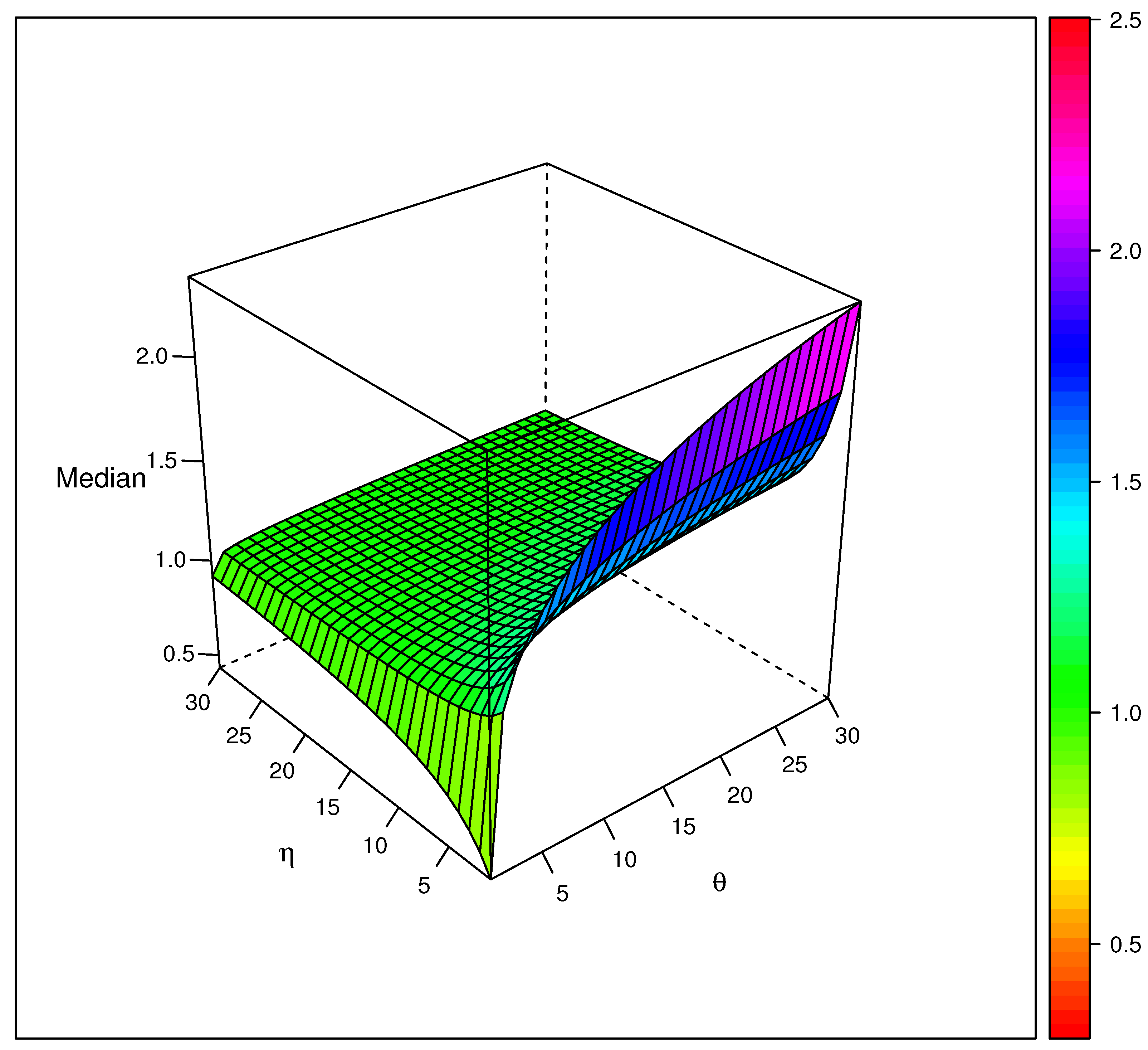
The median of EEP distribution is plotted in Figure 4. Similar to what we observed in Figure 2, the median of an EEP distribution is an increasing function in θ and a decreasing function in η .

3.6. Median Residual Lifetime

For a random variable T, the median residual life time is denoted as MERL ( t ) :
S T ( t + MERL ( t ) ) S T ( t ) = 1 2 ,
where S T ( t ) is the survival function of T. Therefore, by utilizing Equation (15), we have the following:
MERL T ( t | θ , η ) = 2 c θ α 1 c c e α + 1 θ t η 1 α η t t < θ 1 η 2 1 η α t t t θ 1 η .
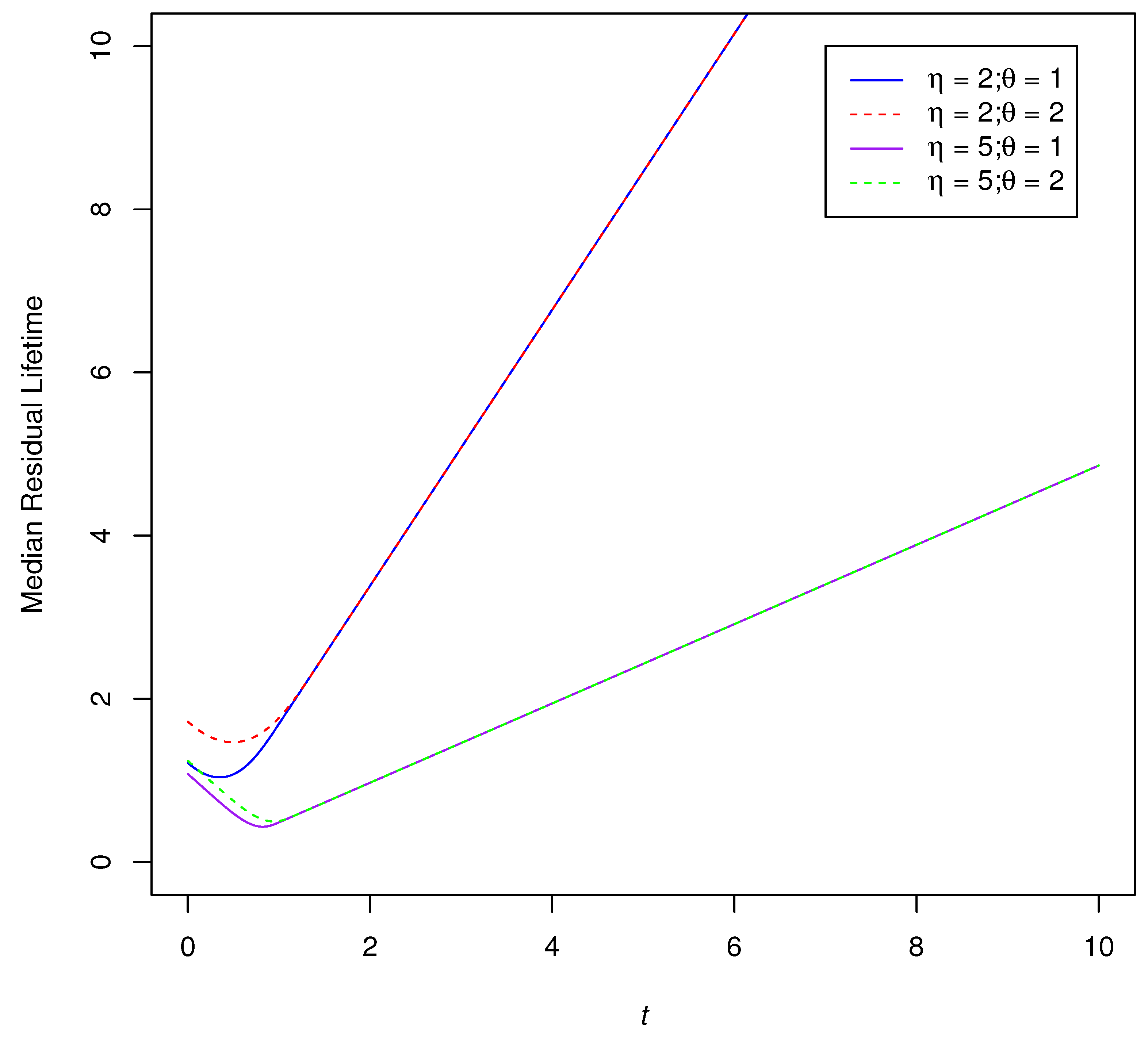
MERL is a very important dynamic measure for distributions with heavy tails. The median residual lifetime functions for selected values of parameters are illustrated in Figure 5. Essentially, if two EEP models have the same value for the parameter η , they will have the same median residual lifetime if t is large.

4. Parameter Estimation

Parameter Search for Two-Parameter EEP Distributions

Suppose that t = ( t 1 , t 2 , , t n ) is an independent identically distributed (i.i.d.) EEP sample with parameters θ and η . Without loss of generality, assume t 1 < t 2 < < t n . Assume that there exists a positive integer m such that t m < θ 1 η < t m + 1 . The corresponding log-likelihood of t can be written as follows:
l ( θ , η ; t ) = n ln ( c ) + n ln ( η ) + m ln ( α + 1 ) + ( n m ) ln ( α ) + ( η 1 ) i = 1 m ln ( t i ) ( α η + 1 ) j = m + 1 n ln ( t j ) + α n ln ( θ ) [ ( α + 1 ) m ] ln ( θ ) α + 1 θ i = 1 m t i η
Due to the existence of the location parameters ( θ and η ) in the EEP model, the maximum likelihood estimates (MLE) of the model parameters cannot be obtained directly by maximizing the log-likelihood function l ( θ , η ; t ) . Liu and Ananda [13,14] introduced a grid-search algorithm to find the estimates of the model parameters. In fact, the estimates can also be obtained by utilizing the ’optim’ function in R. The steps for finding MLE of the model parameters are as follows:
  • Arrange the observations in the sample in increasing order such that t ( 1 ) t ( 2 ) t ( n ) .
  • For m = 1 , 2 , , n 1 , maximize the objective function l ( θ , η ; t ) and obtain ( θ ^ 1 , η ^ 1 ) , ( θ ^ 2 , η ^ 2 ) , , ( θ ^ n 1 , η ^ n 1 ) correspondingly.
  • Start from m = 1 , check the condition t ( 1 ) < ( θ ^ 1 ) 1 η ^ 1 < t ( 2 ) . If this is true, then θ ^ 1 and η ^ 1 are the estimates for θ and η . If not, go to the next step.
  • For m = 2 , check the condition t ( 2 ) < ( θ ^ 2 ) 1 η ^ 2 < t ( 3 ) . If this is true, then θ ^ 2 and η ^ 2 are the estimates for θ and η . Repeat this procedure until the correct m is detected. With the correct m, the corresponding θ ^ m and η ^ m are the estimates for θ and η .
The above algorithm is used to compute the parameter estimates of EEP in the next section.

5. Goodness-of-Fit Tests with Simulation Studies

In this section, we introduce two goodness-of-fit (GoF) tests to assess the GoF of the EEP distribution against its parent distribution, EP distribution. The corresponding hypothesis to be tested is as follows:
H 0 : η = 1 i . e . , data follow an EP ( θ ) H 1 : η 1 i . e . , data follow an EEP ( θ , η ) .
The MLE of θ and η of an EEP distribution can be obtained numerically using the proposed algorithm. Thus, the likelihood ratio test (LRT) could be utilized to test the above hypothesis. Assume that the likelihood function l ( θ , η | t ) takes the form in (17). The LRT statistic λ for the given hypothesis is as follows:
λ = 2 sup θ R + l ( θ , η = 1 ; t ) 2 sup θ R + , η R + l ( θ , η | t ) ,
where λ follows a χ 2 distribution with a degree of freedom 1.
As an alternative procedure, the asymptotic Wald’s test could also be used to test the hypothesis, given the Fisher information matrix and MLE of θ and η . Consider Θ = ( θ , η ) . The Fisher information matrix was derived by Liu and Ananda [13,14] as follows:
I ( Θ ) = 2 l ( θ , η ; t ) θ 2 2 l ( θ , η ) ; t θ η 2 l ( θ , η ; t ) θ η 2 l ( θ , η ; t ) η 2 = I 11 I 12 I 21 I 22 ,
where
I 11 = α n ( α + 1 ) m θ 2 + 2 ( α + 1 ) θ 3 i = 1 m t i η I 12 = α + 1 θ 2 i = 1 m t i η ln ( t i ) I 21 = α + 1 θ 2 i = 1 m t i η ln ( t i ) I 22 = n η 2 + α + 1 θ i = 1 m t i η [ ln ( t i ) ] 2 .
Essentially, the expected value E ( I ( θ ) ) is the Fisher information matrix I ( Θ ) .
Consider Θ ^ = ( θ ^ , η ^ ) as the MLE for Θ = ( θ , η ) . By the asymptotic property of MLE, we have the following under appropriate regularity conditions:
( Θ ^ Θ ) D N ( 0 2 , I 1 ( Θ ) ) , as n ,
where I ( Θ ) stands for the Fisher information matrix of Θ , D represents convergence in distribution, and N ( 0 2 , I 1 ( Θ ) ) is the bivariate normal distribution with covariance matrix I 1 ( Θ ) .
However, in reality, I ( Θ ) = E ( I ( θ ) ) cannot be easily evaluated. Therefore, the observed Fisher information matrix I ( Θ ^ ) is used as a substitute.
I ( Θ ^ ) = I ^ 11 I ^ 12 I ^ 21 I ^ 22 ,
where,
I ^ 11 = α n ( α + 1 ) m θ ^ 2 + 2 ( α + 1 ) θ ^ 3 i = 1 m t i η ^ I ^ 12 = α + 1 θ ^ 2 i = 1 m t i η ^ ln ( t i ) I ^ 21 = α + 1 θ ^ 2 i = 1 m t i η ^ ln ( t i ) I ^ 22 = n η ^ 2 + α + 1 θ ^ i = 1 m t i η ^ [ ln ( t i ) ] 2 .
Correspondingly, I 1 ( Θ ^ ) can be obtained as follows:
I 1 ( Θ ^ ) = 1 I ^ 11 I ^ 22 I ^ 12 I ^ 21 I ^ 22 I ^ 12 I ^ 21 I ^ 11
Since the hypothesis of interest is only involved with the parameter η , we could carry out the Wald’s test procedure easily with the following test statistic:
W = η ^ 1 Var ( η ^ ) ,
where, from (16) and (17), Var ( η ^ ) = I ^ 11 I ^ 11 I ^ 22 I ^ 12 I ^ 21 .
We conducted the simulations to assess the type 1 error performances and the power performances of both tests under different scenarios. For all the simulation scenarios, r = 10,000 samples were generated from the EEP density provided in (11). The R package ‘mistr’ [25] was utilized to generate the random samples.
To evaluate the Type 1 error rates of the two GoF tests, we designed twelve different simulation scenarios with different θ values and sample sizes. The details of the simulation scenarios are listed in Table 1. Table 1 shows the type 1 error performance of both tests under twelve different scenarios. We noticed that both tests can control the type 1 error rate well for all the simulation scenarios.
To assess the power performances of the two GoF tests, we designed various simulation scenarios. The simulation scenarios are described as follows:
  • Three different sample sizes: n = 50 , 100 , 200 .
  • Four different true θ values: θ = 0.01 , 0.1 , 1 , 10 .
  • Eleven true η values: η = 0.5 , 0.6 , 0.7 , 0.8 , 0.9 , 1 , 1.1 , 1.2 , 1.3 , 1.4 , 1.5 .
In total, we generated 132 simulation scenarios.
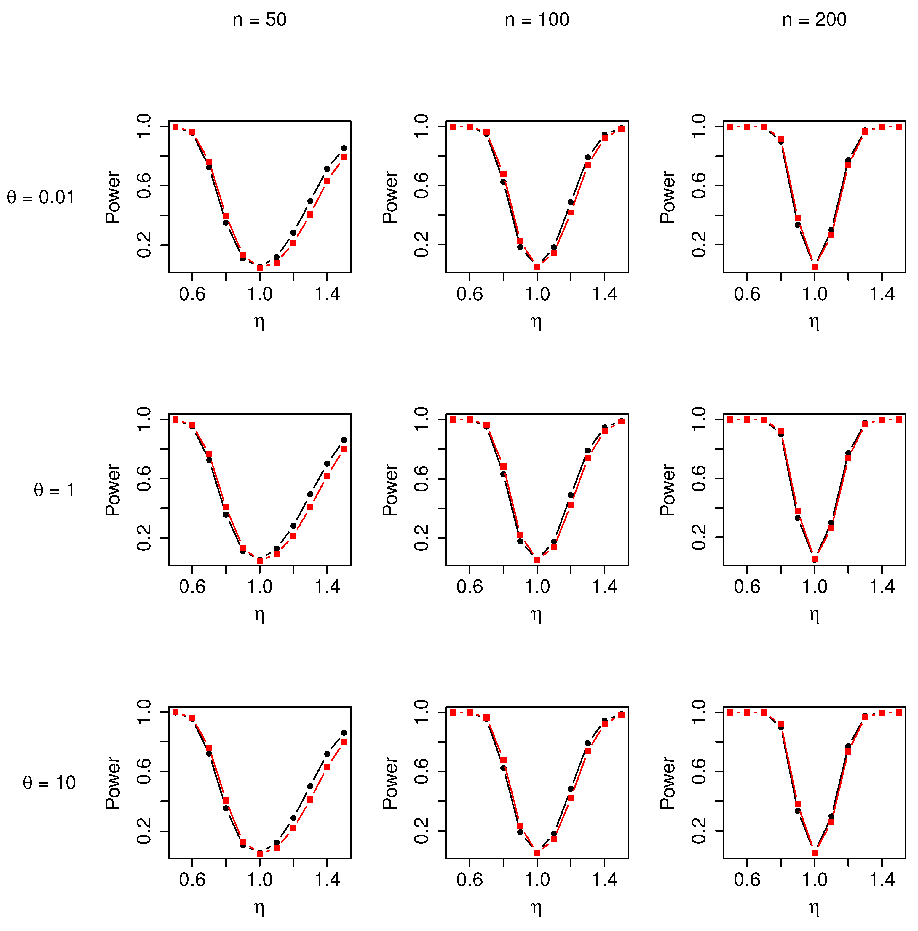
The power comparison of two tests are provided in Figure 6. It can be observed that the power of the tests drops when η increases from 0.5 to 1 and rises when η increases from 1 to 1.5. When the sample size becomes larger, the power of the tests increases. It is also noteworthy that, when the sample size is 50 or 100, the power of the LRT was slightly better than Wald’s test. When the sample size increases to 200, both tests demonstrated similar performance. However, the value of θ did not affect the power of both tests significantly, under all the simulation scenarios.

6. Application to Real Data

In this section, we applied the EEP model to three real data sets to assess its ability in fitting reliability data. For comparison, we choose two models with Pareto tails. The first one is the modified heavy-tailed Pareto model [26]. This is a model that was recently developed to fit the data with UBT-shaped hazard rates. The other one is the Weibull–Pareto composite model [20,23]. This model was previously used to model unimodal survival and reliability data.
We compared the performance of the proposed EEP model against the original EP model, generalized in terms of Akaike information criterion (AIC) [27], AIC3 [28], corrected Akaike information criterion (AICc) [29], and consistent Akaike information criterion (cAIC) [30]. In addition, to justify that the EEP model is proper compared to its parent EP model, LRT and Wald’s test were conducted with the hypothesis in (18). In addition, the Kolmogorov–Smirnoff (KS) test was used to assess the goodness-of-fit of the EEP and the EP model.

6.1. Second Reactor Pump Data

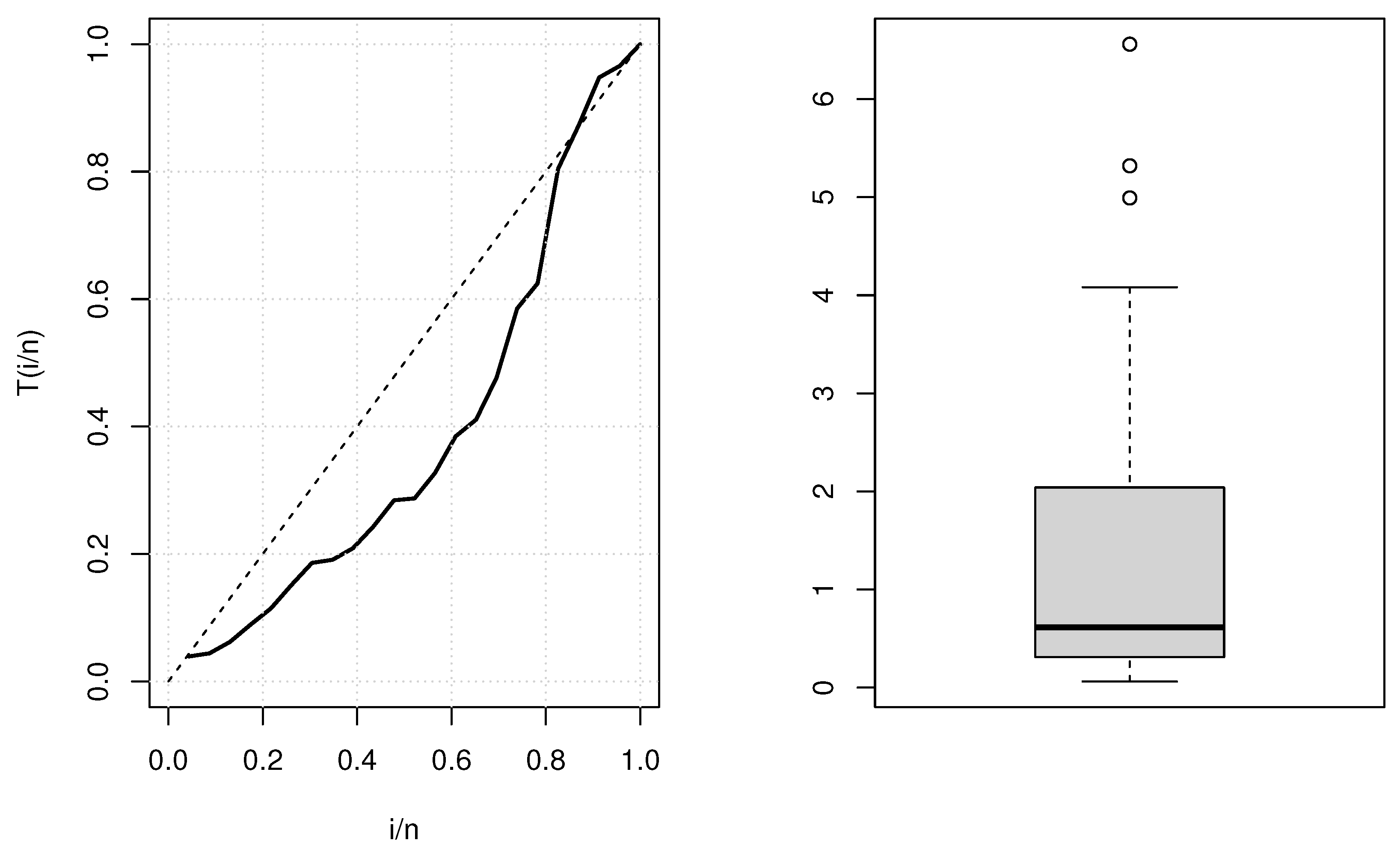
We utilized a data set that describes the time between failure of secondary reactor pumps [31]. The data set is illustrated in Table 2. It was used by previous researchers [6], and it is considered to be a data set that has a upside-down bathtub-shaped hazard rate. The TTT plot and the box plot are presented in Figure 7. The box plot suggests that the data are heavily right-skewed. The TTT plot suggests that the data are associated with a UBT hazard function.
Table 3 presented the estimates with corresponding standard errors, LRT test statistic, Wald test statistic, and corresponding p-values from both tests. We were able to reject the null hypothesis for both of the tests at the significance level α = 0.05 . Thus, we concluded that EEP is more proper compared to EP when fitting to the data set. The KS test also suggested that we could not reject the null hypothesis of the data being from an EEP distribution.
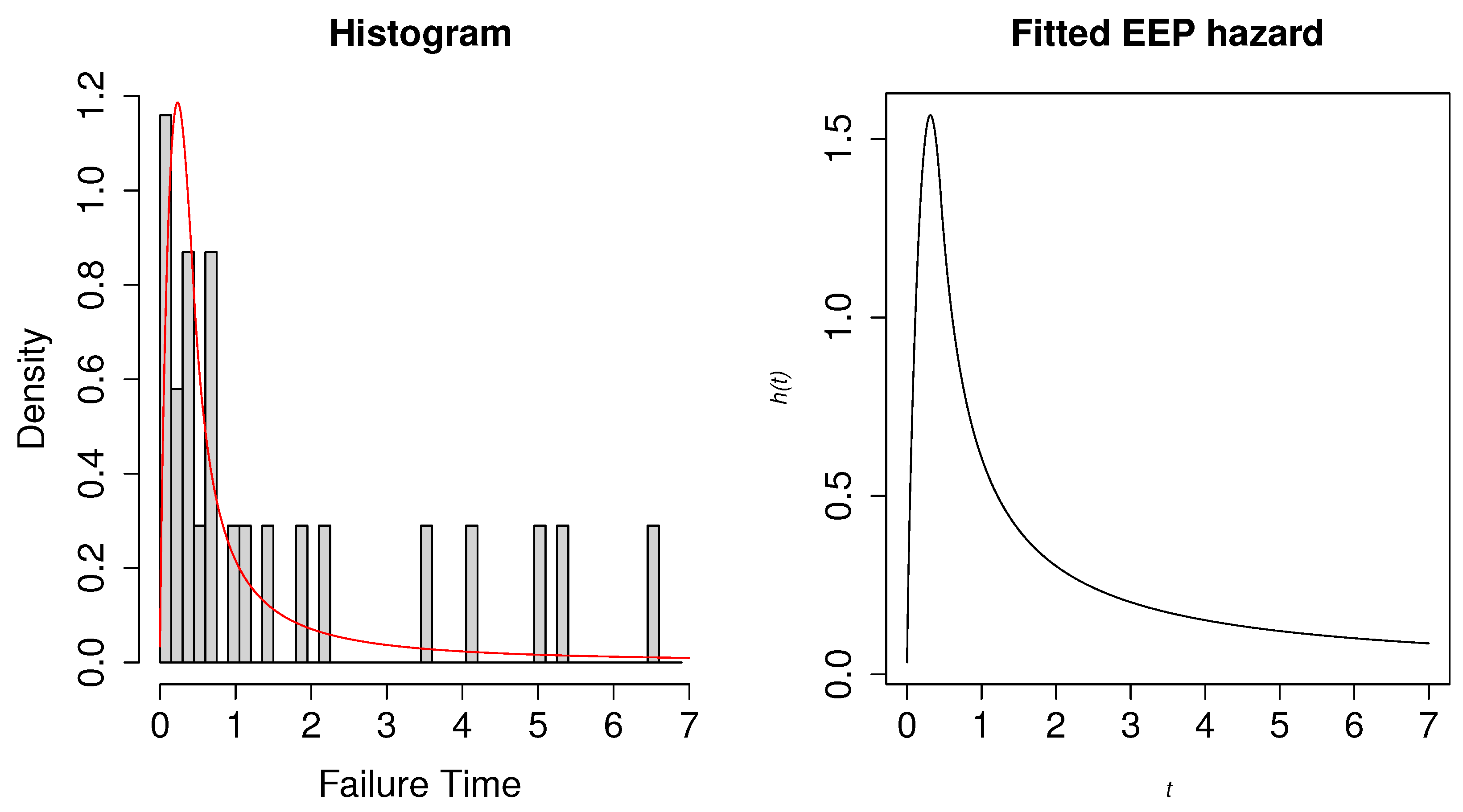
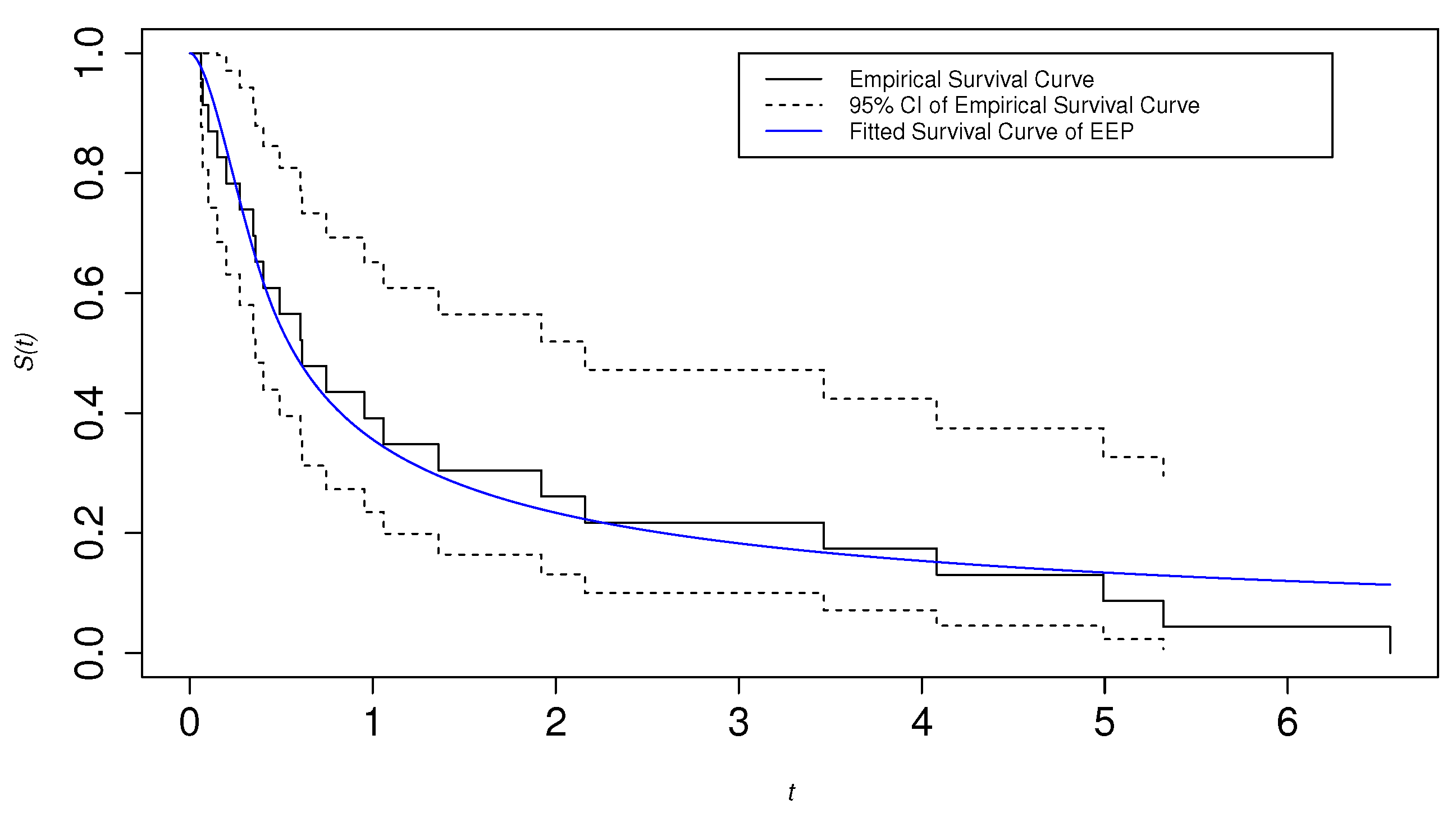
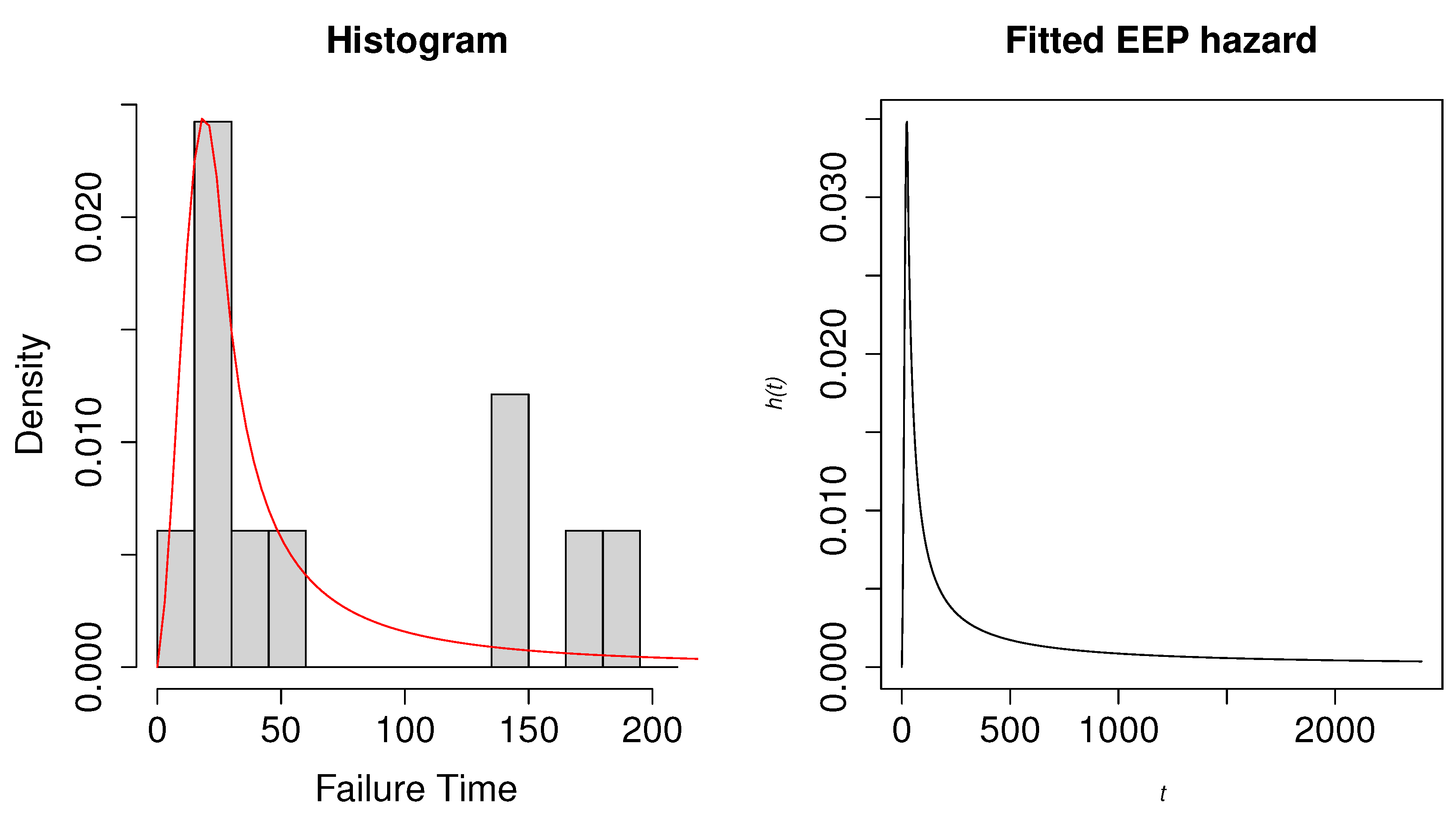
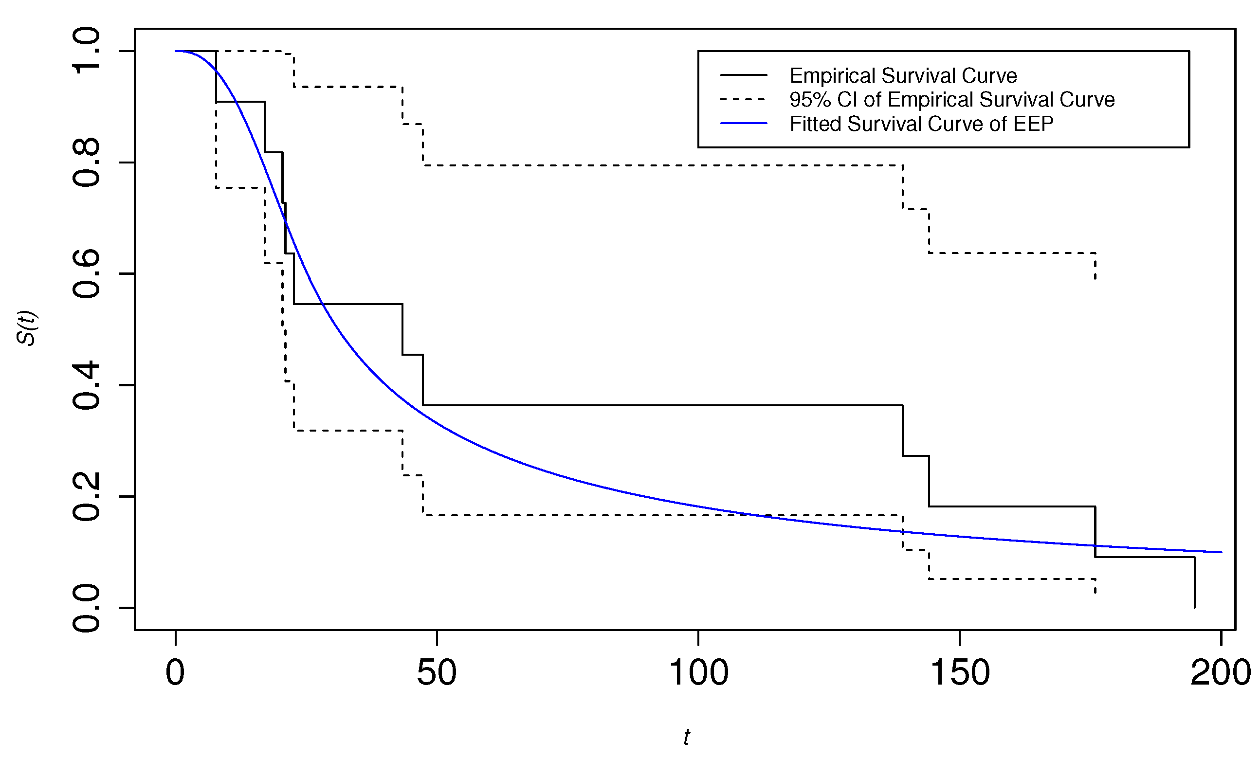
A comparisons of the four different models is presented in Table 4. In terms of all GoF measures, the EEP model demonstrated better performances compared to the original EP model. Moreover, the EEP model presented comparable performances against the heavy-tailed Pareto model and the Weibull–Pareto model, with less parameters. This essentially suggests that the EEP model is capable of explaining the data features with only two parameters. Figure 8 contains the plot-fitted EEP hazard function and the histogram with the fitted pdf. The fitted hazard function possesses a UBT shape. Figure 9 demonstrates a comparison of the empirical survival function and the fitted EEP survival function. It can be clearly seen that EEP provided great performance when fitting to the second reactor pump data set.

6.2. Electrical Breakdown of An Insulating Fluid

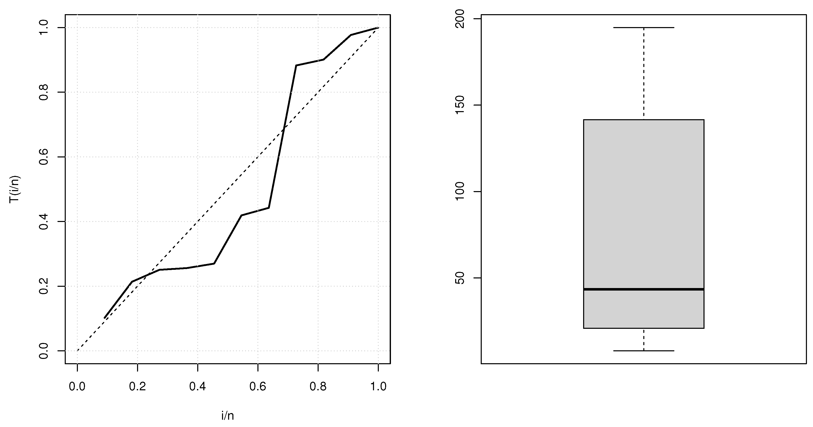
We also utilized the time to electrical breakdown of insulating fluid data [32] to assess the performance of the EEP model. In our analysis, we chose the data set with a test voltage 30 kV. Table 5 illustrates the time to electrical breakdown in terms of hours. Figure 10 consists of the TTT plot and the box plot of the data set. The box plot suggests that the data are right-skewed. The TTT plot confirms that the data are associated with a UBT hazard function.
The estimates, LRT test statistic, Wald test statistic, and corresponding p-values from both tests are presented in Table 6. We were able to reject the null hypothesis for both of the tests at the significance level α = 0.05 . Thus, we concluded that EEP is better compared to EP when fitting to the data set. In addition, the KS test also suggested that we could not reject the null hypothesis of the data being from an EEP distribution at the level of α = 0.05 , while we rejected the null hypothesis of the data being from an EP distribution.
Table 7 summarizes the comparison of the four models in terms of all GoF measures. Compared to the original EP model, the EEP model performed better in terms of all the measures. Moreover, the EEP model demonstrated better performance compared to the three-parameter generalized heavy-tailed Pareto model and the four-parameter Weibull–Pareto model. This implies that the EEP model has better abilities to explain the data with only two parameters. Figure 11 consists of the plot-fitted EEP hazard function and the histogram with the fitted pdf. The fitted hazard function has a UBT shape. Figure 12 presents the comparison of the empirical survival function and the fitted EEP survival function.

7. Concluding Remark and Future Work

In this paper, we introduced a special member from the generalized family of exponentiated composite distributions, named exponentiated exponential-Pareto distribution. We derived the properties of this distribution including the moments, the survival function, the hazard function, and the quantile function. We also discussed the parameter estimation and the goodness-of-fit tests for this distribution against its parent distribution. Limited simulations were conducted to compare the performances of the goodness-of-fit tests. In the section with a real data analysis, the proposed distribution demonstrated great performance when fitted to specific reliability data sets with hazard rates being upside-down bathtub-shaped. We hope that this new model can provide different insights into reliability data modeling. Since we only studied one special distribution from the family of generalized exponentiated composite distributions in this paper, the exploration of more special distributions from this family is warranted.

Author Contributions

Conceptualization, B.L. and M.M.A.A.; methodology, B.L. and M.M.A.A.; software, B.L.; validation, B.L. and M.M.A.A.; formal analysis, B.L.; investigation, B.L. and M.M.A.A.; resources, B.L.; writing—original draft preparation, B.L.; writing—review and editing, B.L. and M.M.A.A.; supervision, M.M.A.A.; project administration, B.L. and M.M.A.A.; All authors have read and agreed to the published version of the manuscript.

Funding

This research received no external funding.

Data Availability Statement

All data related to this study are publicly available.

Acknowledgments

We appreciate the help and the comments from the reviewers and the editors.

Conflicts of Interest

The authors declare no conflict of interest.

Abbreviations

The following abbreviations are used in this manuscript:
UBTUpside-down bathtub-shaped
GECGeneralized exponentiated composite distributions
pdfProbability density function
CDFCumulative distribution function
EPExponential-Pareto distribution
EEPExponentiated exponential-Pareto distribution
LRTLikelihood ratio test
MLEMaximum likelihood estimates
AICAkaike information criterion
BICBayesian information criterion
AICcCorrected Akaike information criterion
cAICConsistent Akaike information criterion
KSKolmogorov–Smirnoff

References

  1. Bennett, S. Log-Logistic Regression Models for Survival Data. J. R. Stat. Soc. Ser. C (Appl. Stat.) 1983, 32, 165–171. [Google Scholar] [CrossRef]
  2. Prentice, R.L. Exponential Survivals with Censoring and Explanatory Variables. Biometrika 1973, 60, 279–288. [Google Scholar] [CrossRef]
  3. Prentice, R.L. Linear Rank Tests with Right Censored Data. Biometrika 1978, 65, 167–179. [Google Scholar] [CrossRef]
  4. Efron, B. Logistic Regression, Survival Analysis, and the Kaplan-Meier Curve. J. Am. Stat. Assoc. 1988, 83, 414–425. [Google Scholar] [CrossRef]
  5. Langlands, A.O.; Pocock, S.J.; Kerr, G.R.; Gore, S.M. Long-term survival of patients with breast cancer: A study of the curability of the disease. Br. Med. J. 1979, 2, 1247–1251. [Google Scholar] [CrossRef] [PubMed] [Green Version]
  6. Sharma, V.K.; Singh, S.K.; Singh, U. A new upside-down bathtub shaped hazard rate model for survival data analysis. Appl. Math. Comput. 2014, 239, 242–253. [Google Scholar] [CrossRef]
  7. de Gusmão, F.R.S.; Ortega, E.M.M.; Cordeiro, G.M. The generalized inverse Weibull distribution. Stat. Pap. 2011, 52, 591–619. [Google Scholar] [CrossRef]
  8. Khan, M.S.; King, R. A New Class of Transmuted Inverse Weibull Distribution for Reliability Analysis. Am. J. Math. Manag. Sci. 2014, 33, 261–286. [Google Scholar] [CrossRef]
  9. Domma, F.; Condino, F.; Popović, B.V. A new generalized weighted Weibull distribution with decreasing, increasing, upside-down bathtub, N-shape and M-shape hazard rate. J. Appl. Stat. 2017, 44, 2978–2993. [Google Scholar] [CrossRef]
  10. Sharma, V.K.; Singh, S.K.; Singh, U.; Agiwal, V. The inverse Lindley distribution: A stress-strength reliability model with application to head and neck cancer data. J. Ind. Prod. Eng. 2015, 32, 162–173. [Google Scholar] [CrossRef]
  11. Sharma, V.K.; Singh, S.K.; Singh, U.; Merovci, F. The generalized inverse Lindley distribution: A new inverse statistical model for the study of upside-down bathtub data. Commun. Stat. Theory Methods 2016, 45, 5709–5729. [Google Scholar] [CrossRef]
  12. Maurya, S.; Singh, S.; Singh, U. A New Right-Skewed Upside Down Bathtub Shaped Heavy-tailed Distribution and its Applications. J. Mod. Appl. Stat. Methods 2021, 19, eP2888. [Google Scholar] [CrossRef]
  13. Liu, B.; Ananda, M.M.A. Analyzing insurance data with an exponentiated composite Inverse-Gamma Pareto Model. Commun. Stat. Theory Methods 2022. [Google Scholar] [CrossRef]
  14. Liu, B.; Ananda, M.M.A. A Generalized Family of Exponentiated Composite Distributions. Mathematics 2022, 10, 1895. [Google Scholar] [CrossRef]
  15. Scollnik, D.P.M. On composite lognormal-Pareto models. Scand. Actuar. J. 2007, 2007, 20–33. [Google Scholar] [CrossRef]
  16. Cooray, K.; Ananda, M.M.A. Modeling actuarial data with a composite lognormal-Pareto model. Scand. Actuar. J. 2005. [Google Scholar] [CrossRef]
  17. Teodorescu, S.; Vernic, R. A composite Exponential-Pareto distribution. Ann. “Ovidius” Univ. Constanta Math. Ser. 2006, XIV, 99–108. [Google Scholar]
  18. Teodorescu, S.; Vernic, R. Some Composite ExponentialPareto Models for Actuarial Prediction. J. Econ. Forecast. 2009, 12, 82–100. [Google Scholar]
  19. Preda, V.; Ciumara, R. On Composite Models: Weibull-Pareto and Lognormal-Pareto. A comparative study. J. Econ. Forecast. 2006, 3, 32–46. [Google Scholar]
  20. Cooray, K. The Weibull–Pareto Composite Family with Applications to the Analysis of Unimodal Failure Rate Data. Commun. Stat. Theory Methods 2009, 38, 1901–1915. [Google Scholar] [CrossRef]
  21. Deng, M.; Aminzadeh, M.S. Bayesian predictive analysis for Weibull-Pareto composite model with an application to insurance data. Commun. Stat. Simul. Comput. 2022, 51, 2683–2709. [Google Scholar] [CrossRef]
  22. Aminzadeh, M.S.; Deng, M. Bayesian predictive modeling for Inverse Gamma-Pareto composite distribution. Commun. Stat. Theory Methods 2019, 48, 1938–1954. [Google Scholar] [CrossRef]
  23. Grün, B.; Miljkovic, T. Extending composite loss models using a general framework of advanced computational tools. Scand. Actuar. J. 2019, 2019, 642–660. [Google Scholar] [CrossRef]
  24. Nadarajah, S. Exponentiated Pareto distributions. Statistics 2005, 39, 255–260. [Google Scholar] [CrossRef]
  25. Sablica, L.; Hornik, K. mistr: A Computational Framework for Mixture and Composite Distributions. R J. 2020, 12, 283–299. [Google Scholar] [CrossRef]
  26. Shrahili, M.; Kayid, M. Modeling extreme value data with an upside down bathtub-shaped failure rate model. Open Phys. 2022, 20, 484–492. [Google Scholar] [CrossRef]
  27. Burnham, K.P.; Anderson, D.R. Model Selection and Multimodel Inference, 2nd ed.; Springer: New York, NY, USA, 2002. [Google Scholar]
  28. Bozdogan, H. Mixture-Model Cluster Analysis Using Model Selection Criteria and a New Informational Measure of Complexity. In Proceedings of the First US/Japan Conference on the Frontiers of Statistical Modeling: An Informational Approach: Volume 2 Multivariate Statistical Modeling; Bozdogan, H., Sclove, S.L., Gupta, A.K., Haughton, D., Kitagawa, G., Ozaki, T., Tanabe, K., Eds.; Springer: Dordrecht, The Netherlands, 1994; pp. 69–113. [Google Scholar] [CrossRef]
  29. Hurvich, C.M.; Tsai, C.L. Regression and time series model selection in small samples. Biometrika 1989, 76, 297–307. [Google Scholar] [CrossRef]
  30. Bozdogan, H. Model selection and Akaike’s Information Criterion (AIC): The general theory and its analytical extensions. Psychometrika 1987, 52, 345–370. [Google Scholar] [CrossRef]
  31. Suprawhardana, M.S.; Sangadji, P. Total Time on Test Plot Analysis for Mechanical Components of the Rsg-Gas Reactor. Atom Indones 1999, 25, 81–90. [Google Scholar]
  32. Meeker, W.Q.; Escobar, L.A.; Pascual, F.G. Statistical Methods for Reliability Data; John Wiley & Sons: Hoboken, NJ, USA, 2022. [Google Scholar]
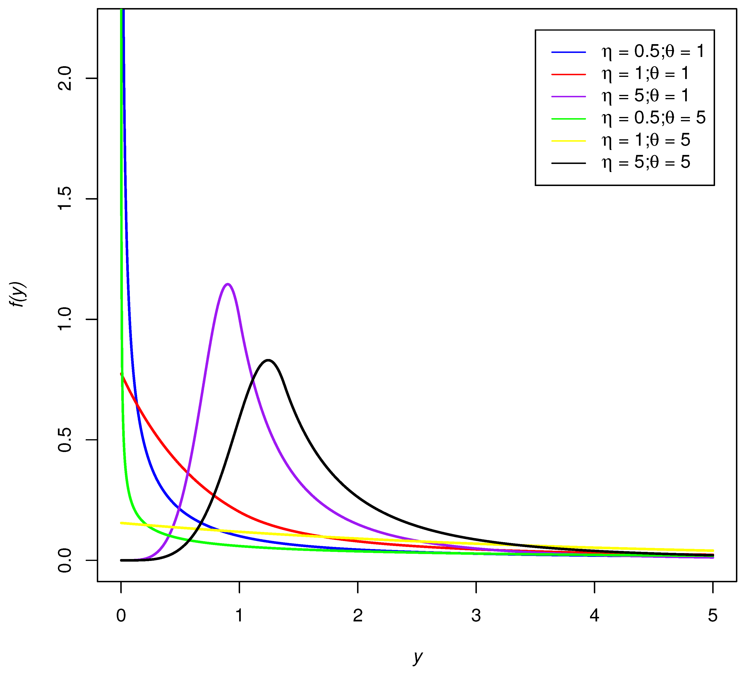
Figure 1. The pdf of an EEP distribution with different parameters.
Applsci 13 00645 g001
Figure 2. Mean plot of an EEP distribution with different parameters.
Applsci 13 00645 g002
Figure 3. Hazard function of an EEP distribution with different parameters.
Applsci 13 00645 g003
Figure 4. Median plot of EEP distribution with different parameters.
Applsci 13 00645 g004
Figure 5. The median residual lifetime function plot of EEP distribution with different parameters.
Applsci 13 00645 g005
Figure 6. Power comparison of the Likelihood ratio test and asymptotic Wald’s test (the red line represents the asymptotic Wald’s test, and the black line represents the LRT).
Applsci 13 00645 g006
Figure 7. TTT plot (left) and box plot (right) of the second reactor pump data set.
Applsci 13 00645 g007
Figure 8. Fitted hazard function of EEP distribution for secondary reactor pumps data set.
Applsci 13 00645 g008
Figure 9. Fitted EEP survival curve for secondary reactor pumps data set.
Applsci 13 00645 g009
Figure 10. TTT plot (left) and box plot (right) of the time to electric breakdown data set.
Applsci 13 00645 g010
Figure 11. The fitted hazard function of EEP distribution for the time to electric breakdown data set.
Applsci 13 00645 g011
Figure 12. Fitted EEP survival curve for time to electric breakdown data set.
Applsci 13 00645 g012
Table 1. Type 1 error rates for likelihood ratio test and asymptotic Wald’s test.
θ Sample
Size (n)
LRTWald’s Test
α = 0 . 01 α = 0 . 05 α = 0 . 01 α = 0 . 05
0.01 n = 50 0.01100.05360.01070.0484
n = 100 0.01250.04960.01050.0477
n = 200 0.00950.04990.01010.0503
0.1 n = 50 0.00940.05140.00870.0443
n = 100 0.01080.05290.01040.0519
n = 200 0.01120.04950.01130.0517
1 n = 50 0.01160.05370.01110.0469
n = 100 0.01200.05420.01210.0523
n = 200 0.01000.04840.01130.0508
10 n = 50 0.01200.05440.00950.0490
n = 100 0.01040.05230.01030.0495
n = 200 0.01210.05180.01270.0523
Table 2. Second reactor pump failure time data.
2.160, 0.150, 4.082, 0.746, 0.358, 0.199, 0.402, 0.101, 0.605, 0.954,
1.359, 0.273, 0.491, 3.465, 0.070, 6.560, 1.060, 0.062, 4.992, 0.614,
5.320, 0.347, 1.921
Table 3. Summary of the EEP and EP fit to the second reactor pump data set.
ModelEstimatesLRT Statistic
(p-Value)
Wald Statistic
(p-Value)
KS Statistic
(p-Value)
EEP θ = 0.25516
η = 1.73300
6.32602
(0.01190)
4.45271
(0.03485)
0.13043
(0.9924)
EP θ = 0.60707 --0.26087
(0.4218)
Table 4. Comparison of the four models in terms of the five GoF measures.
ModelpAICAIC3AICcCAIC
EEP272.2952874.2952872.8952876.56627
EP176.6213077.6213076.8117878.75679
Generalized Heavy-Tailed Pareto369.8628872.8628871.1260476.26936
Weighted Weibull–Pareto Composite469.7153273.7336871.9559078.27566
Table 5. Time to electric breakdown data.
7.74, 17.05, 20.46, 21.02 22.66, 43.40,
47.30, 139.07 144.12, 175.88, 194.90
Table 6. Summary of the EEP and EP fit to the time to electric breakdown set.
ModelEstimatesLRT Statistic
(p-Value)
Wald Statistic
(p-Value)
KS Statistic
(p-Value)
EEP θ = 3326.133
η = 2.473841
4.08993
(0.04314)
7.090596
(0.008)
0.54545
(0.0758)
EP θ = 41.39566 --0.90909
(0.0002254)
Table 7. Comparison of the four models in terms of the five GoF measures.
ModelpAICAIC3AICcCAIC
EEP2121.6466123.6466123.1466124.4424
EP1126.7372127.7372127.1816128.1351
Generalized Heavy-Tailed Pareto3123.4848125.2912125.7197126.4848
Weighted Weibull–Pareto Composite4125.2129129.2129131.8795130.8045
Disclaimer/Publisher’s Note: The statements, opinions and data contained in all publications are solely those of the individual author(s) and contributor(s) and not of MDPI and/or the editor(s). MDPI and/or the editor(s) disclaim responsibility for any injury to people or property resulting from any ideas, methods, instructions or products referred to in the content.