Modeling the Data Provenance of Relational Databases Supporting Full-Featured SQL and Procedural Languages

Abstract

Data provenance is information about where data come from (provenance data) and how they transform (provenance transformation). Data provenance is widely used to evaluate data quality, trace errors, audit data, and understand references among data. Current studies on data provenance in relational database management systems (RDBMS) still have limitations in supporting full-featured SQL or procedural languages. With these challenges in mind, we present a formal definition of provenance data and provenance transformation for relational data. Then, we propose a solution to support data provenance in relational databases, including provenance graphs and provenance routes. Our method not only solves the complicated problem of modeling provenance in DBMS but also is capable of extending procedural languages in SQL. We also present ProvPg, a PostgreSQL-based prototype database system supporting data provenance in multiple granularities. ProvPg implements extraction, calculation, query, and visualization of provenance. We perform TPC-H tests for ProvPg and PostgreSQL, respectively. Experimental results show that ProvPg addresses the vision of supporting data provenance with little extra computation overhead for the execution engine, which indicates that our model is applicable to lineage tracing applications.

1. Introduction

Most data in applications are generated by a series of computations and transformations on the native data, making it difficult to trace the source. For example, SwissProt and Wikipedia are curated databases, and their contents are derived or edited from other sources, including curated databases. However, applications, such as scientific computing [1], data warehouse [2], grid-computing [3], curated databases [4], data flow management [5], and copyright management [6], are very concerned with data provenance, which refers to the origin, lineage, or source of data, which is essential for assessing data quality, as well as understanding the lineage and dependencies between data.

In relational databases, data are represented as relational tables, fields, tuples, or attribute values in terms of granularity. The creation and transformation of data depend on operations in the database management process, including the execution of SQL or stored procedural languages and the importing of external data. Adding the following functions to database management system (DBMS) helps to improve the usability of supporting data provenance in DBMS: (i) extracting provenance information (including provenance data and provenance transformation) in the data management process; (ii) supporting data provenance information at different levels of granularity; and (iii) supporting the full-featured SQL, stored procedure, and even other script languages for data processing in the real-life application scenarios. All of these functions play a crucial role in data interpretation, data debugging, and troubleshooting, which will efficiently enhance the data analysis capabilities of the database system.

However, existing research in relational data provenance is insufficient in supporting provenance in DBMS. The main challenges are: (i) Few studies support the relational data provenance of multiple granularities simultaneously. The current provenance system captures provenance information in coarse granularity using schema-based or fine granularity, such as tuple-based and value-based, and the coexistence of multi-granularity provenance in the same system lacks efficient models and methods. For example, many workflow systems supporting data provenance attach provenance information to coarse-grained files [7,8,9,10], while other customized systems attach provenance information to fine-grained attribute values [11,12,13]. (ii) Tuple-level and value-level data provenance attract more research than data transformation [14,15]. Despite their significant application value, systems based on these studies have limitations in many aspects, for example, the inconvenience of comprehensively understanding data provenance relation (especially the data transformation process). (iii) Few database systems provide support for data provenance except DBNotes [14], pSQL [16], ORCHESTRA [17], and ProvSQL [18]. Furthermore, a large percentage of studies are based on lineage [19,20], why-provenance, where-provenance [21], how-provenance [22], and other theories. For the convenience of theoretical research, they are confined to a simple SQL, whereas there are many complex SQL in practical application scenarios. Glavic [23,24] proposed a provenance representation model of perm-provenance and perm-transformation on the basis of lineage, which can support complex SQL queries. However, the model significantly relies on the SQL syntax structure, making the transformation too redundant and complicated to understand the dependencies between data and extend to languages other than SQL.

To address the above challenges, we present a provenance model that fully supports full-featured SQL and procedural query language. Our model describes data provenance information at multiple levels of relation tables, fields, tuples, and values, especially the provenance transformation process.

The main contributions of this paper are summarized as follows:

• A novel method and model of data provenance are presented. The model describes data provenance information at multiple levels, including relational table schema, attribute fields, tuples, and values. Our model investigates provenance transformation, which has been neglected in previous research.
• Data provenance supporting full-featured SQL and procedural languages is implemented. We combine basic operations, such as the projection and filter to represent provenance transformation, making it possible to support full-featured SQL or even procedural languages.

The rest of this paper is organized as follows. The next section introduces related research on data provenance techniques, Section 3 discusses the semantic representation of the relational data provenance, Section 4 describes the relational data provenance model, and Section 5 concludes the paper.

2. Related Research

Wang et al. [25] first proposed the concept of data provenance and applied it to heterogeneous databases. Earlier research mainly focused on fine-grained (tuple, value). Annotation propagation [26,27] or inverse operation were the typical methods used to track data provenance. Woodruff et al. [28] obtained provenance data by inverting the original query to solve the problems of data volume expansion and computational complexity. Later, Cui et al. [19,20] proposed the lineage approach, which utilized reverse queries to compute tuple-level provenance data and gave the first standardized definition of tuple-level data provenance in the relational database. Based on lineage, Buneman et al. [21] presented the tuple-, field-, and value-level provenance representations, called why-provenance and where-provenance, respectively, to track data provenance from different perspectives. Green et al. [22] introduced a “provenance semiring” structure of provenance representation, called how-provenance. How-provenance canonically explains the generation of tuples and plays a vital role in uncertain databases and computing data credibility. Glavic [23,24] proposed perm-provenance on the basis of lineage, which could adapt to complex SQL queries. In the meantime, perm-transformation was proposed with a relational expression tree structure to describe and compare provenance transformation. The utilization of the rewrite mechanism in provenance queries makes it possible that the query engine simultaneously computes provenance data and query results, along with the optimal utilization of the computation engine and the optimization for calculation efficiency. Lineage, why-, where-, and how-provenance, and extensions and optimizations of previous research [17,29] form the theoretical foundation for subsequent provenance models and applications.

The typical applications of data provenance are: (1) Orchestra [30] is a collaborative data-sharing system based on how-provenance in a P2P environment, which takes advantage of the characteristics of provenance transformation to synchronize data on different ends. (2) DBNotes [14], a system based on where-provenance, tracked provenance information by attaching zero or more notes to every value in a relation and propagating the attached notes to the result of queries. (3) Based on how-provenance, the Trio system [15] quantitatively calculates the credibility of data in the uncertainty database by combining and distilling data provenance and uncertainty theory. (4) SPIDER [31] proposes a method of “Route” as a description of the relationship between source and target data with schema mapping, tracking the transformation process of the target data, which is very useful for understanding and exploring schema mappings.

In recent years, most research built on previous studies and applied them to business contexts. Specifically, research directions include data provenance of distributed systems [32,33,34,35,36], compaction of data provenance information with full-featured query languages [37,38,39,40,41,42], etc. Studies on full-featured query language are intimately related to our study, and we highlight them below: ProvenanceCurious [43] is a tool for inferring data provenance in scripting languages. It demonstrates a provenance graph to represent a view of data dependencies, which helps to debug. This tool is implemented only with Python as the scripting language, without more details or a formal definition of the transformation process. Inspired by the ideas of program slicing and abstract interpretation, Miiller et al. [44] proposed an approach to translate the query language into an abstract Turing complete language (similar to Python), which can compute and track fine-grained (tuple, value) provenance data based on why- and where-provenance. This method embraces any SQL constructs, such as (correlated) sub-queries, recursive common table expressions, and built-in and user-defined functions, which are valuable in real-world database scenarios. Dietrich et al. [45] developed observational debuggers for SQL. These studies show that data lineage no longer solely relies on SQL, Datalog, or simple streaming processes, and the support of procedural languages with control structures is an urgent requirement.

3. Semantic Expression of Relational Data Provenance

Relational data provenance refers to the source of relational schemas or relational data (tables, fields, tuples, values) and all operations involved in changing these data in database management. This section first gives a canonical definition of provenance data based on where-prov and extends it to the tuple-level, called TupWhere-Prov. Then, we define provenance explaining transformation (PET) to introduce provenance transformation in SQL and procedural languages.

3.1. Contribution Semantics

In the view of query, relational schemas or relational data are the results of SQL execution in DBMS, and all inputs are the provenance data of the output. A super coarse-grained provenance has less significance and causes a large amount of provenance data storage. Therefore, separating the normalized data contributed to the output data from the input data as the provenance data represent a more rational approach. Currently, the provenance data research solves the division of provenance by contribution semantics, which includes three categories from a high-level perspective: input contribution semantics, copy contribution semantics, and influence contribution semantics [23]. In the input contribution semantics, all inputs are the provenance data. In the semantics of influence contribution, only the inputs that affect the existence of the outputs are the provenance data, and missing data items of these data will lead to unrecoverable provenance. For copy contribution semantics, only those data items (partial or complete) copied to the output are provenance data. For example, some items are only used for filtering data but not copied to the output. These data are provenance data in influence contribution semantics but are not subject to copy contribution semantics.

The investigation of the provenance transformation process is the evaluation of the contribution semantics of provenance data. This is difficult in data provenance systems as SQL queries and relational algebra operations are transformation units in the transformation process. Input contribution semantics ignore the internal details of transformations, and thus the process is a black box. Unlike input contribution semantics, copy and influence contribution semantics analyze the details of the modifications, and influence semantics contain richer details than copy semantics. However, the influence semantics are complicated and cumbersome for understanding the relationship between data in a complex query language.

Previous studies use how-prov and perm-transformations to express provenance transformation. However, how-prov’s K-relation expression contains little information about the provenance transformation. The relational algebraic expression of perm-transformations, a tree structure that significantly relies on SQL syntax, is complicated and cumbersome for complex queries. Therefore, this paper proposes provenance explaining transformation (PET) to investigate this in more detail. PET begins with several basic operations (such as projection and join), providing the ability to describe conversions in SQL and stored procedures. To eliminate the influence of the complex features of languages, such as SQL, and explain the provenance transformation process concisely and clearly, we choose where-prov, a kind of copy contribution semantics, as the theoretical basis of the provenance data and define PET based on it.

3.2. Terminology and Symbols

In order to facilitate the definition of methods and models, we introduce symbols and the relational algebra used in the subsequent sections.

Let $\varpi$ be a collection of field names (or attribute names) $\left\{A_1,\dots ,A_n\right\}$, U and V are finite subsets of $\varpi$, $D_i\left(i=1,2,\dots ,n\right)$ is a finite domain of attribute $A_i$. A record (or tuple) $t,t_1,t_2,t^{\prime },u,\dots$ is a function $U\to \left\{D_1,\dots ,D_n\right\}$, written as $\left(A_1:D_1,\dots ,A_n:D_n\right)$. Then, $t·A$ is the value of field A, and t[U] restricts the tuple t to fields set $U$.

A relation or table $r:U$ is a finite set of tuples over U. Let $\Re$ be a finite collection of relation names $\left\{R_1,\dots ,R_n\right\}$. A schema R is a mapping $\left(R_1:U_1,\dots ,R_n:U_n\right)$ from $\Re$ to finite subsets of $\varpi$. A database (or instance) $I:\left(R_1:U_1,\dots ,R_n:U_n\right)$ is a function mapping each $R_i:U_i\in \mathit{R}$ to a relation $r_i$ over $U_i$. For relation table $r_i$ and attribute set $A,B,C,\in U_i$, $t\left[A\right]$ is the value of tuple t ($t\subseteq r_i$) on field set A and $r_i\left[A\right]=\left\{t\left[A\right]|t\subseteq r_i\right\}$.

We also define tuple locations as tuples tagged with relation names, written as (R, t). Similarly, field locations are written as a triple (R, t, A). If the context is clear, the triple (R, t, A) is simplified to $\left(R,t\left[A\right]\right)$. Moreover, $t=u\oplus v$ denotes the concatenation of tuple u and v, and the result is tuple t.

Constant data involved in SQL, including constants, constant tuples, such as VALUES (101, ‘abc’), or data in external text files, are uniformly replaced by the notation $\perp$ to minimize the impact of the tedious constant data on the discussion. For instance, $“A+func\left(B,\perp \right)-\perp ”$ is a simplification of “A + func(B, 1) − 2”.

We use the expression Q(I) as a query for a database instance I and for any output tuple $t,t\in Q\left(I\right)$. R(I) is a relational table in the instance I. Particularly, a query is written as Q in the context where the instance I is clear. In query $Q=<q,R>R=\left\{R_1,\dots ,R_n\right\}$, q is the language structure that corresponds to SQL, stored procedural language, and other data processing script languages. $R_i$ is the relational table name involved in the query Q. In particular, $R_i\left(I\right)$ only references the relational table $R_i$.

We use the following notation for (monotone) relational algebra queries:

$$Q\colon\colon =\left\{t\right\}|{\sigma }_{\theta }\left(Q\right)\left|{\pi }_U\left(Q\right)\right|Q_1\infty Q_2\left|Q_1{\displaystyle \cup }{Q}_2\right|{\alpha }_{A,B}\left(Q\right)$$

Here, {t} is a set of constant tuples, and the following symbols denote selection, projections, join (or natural join), union, and group and aggregation operation, respectively. The group and aggregation operation is represented as ${\alpha }_{A,B}\left(Q\right)=g\oplus aggr\left(G{\left[B\right]}^{*}\right)$, where g $=e\left(A\right) \left(A\in G\right)$, e is an expression parameterized by the grouping filed A, g is the set of the output tuples, and $aggr\left(G{\left[B\right]}^{*}\right)$ denotes that the aggregation function $aggr$ that takes the values of tuples in the group G over the aggregation field B as the input. The final output tuples are the concatenation performed on the output result of the calculation expression and aggregation operation.

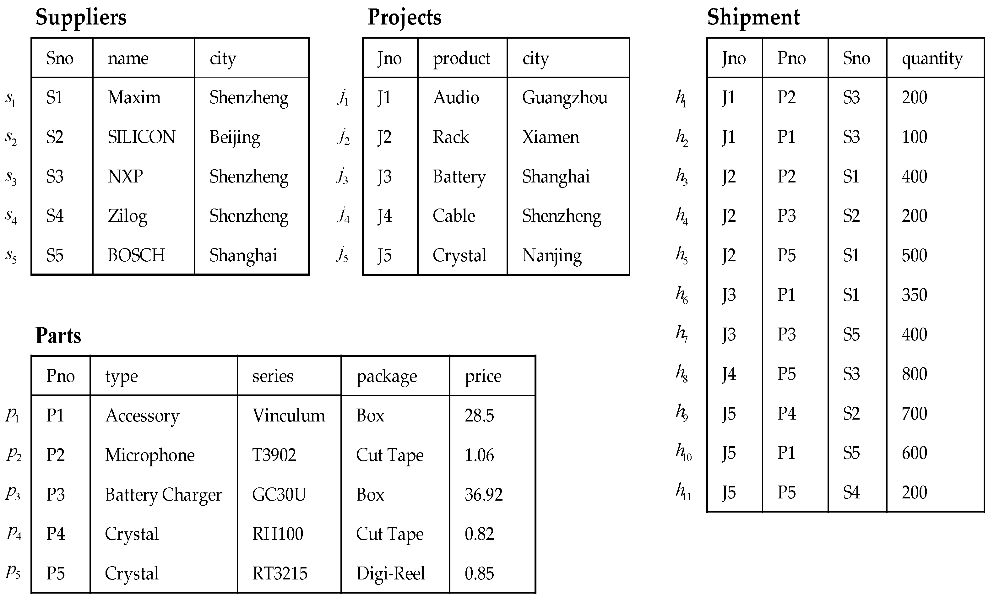
To illustrate the semantics of our method with examples, we considered the suppliers–parts–projects database, reproduced for convenience in Figure 1, where $s_i$, $j_i$, $p_i$, and $h_i$ are used to identify the tuples.

3.3. Representation of Provenance Data

Where-prov is a copy contribution semantics describing the relationship between the inputs and outputs by defining propagation rules of attribute values on algebraic operations. To support full-featured SQL and procedural language queries, we extend the annotation propagation rules of [46] to group aggregation operation and formally define where-provenance on the filter, projection, join, union, and group aggregation operations (See Definition 1).

Hereafter, we consider annotated relations and annotations propagating between locations in the database. Assume that location is denoted as triple $\left(R,t^{\prime },A\right)$, which carries a set of zero or more annotations.

• Selection. For $t\in {\sigma }_{\theta }\left(R\right)$, an annotation on $\left(R,t^{\prime },A\right)$ propagates to $\left({\sigma }_{\theta }\left(R\right),t,A\right)$ if $t=t^{\prime }$.
• Projection. For $t\in {\mathsf{\Pi }}_U\left(R\right)$, an annotation on $\left(R,t^{\prime },A\right)$ propagates to $\left({\mathsf{\Pi }}_U\left(R\right),t,U\right)$, where $U\subseteq A$ and $t=t^{\prime }\left[U\right]$.
• Join. For $t\in R_1\infty R_2$, annotations on $\left(R_1,t_1,A\right)$ and/or $\left(R_2,t_2,A\right)$ propagate to $\left(R_1\infty R_2,t,A\right)$, where $t\left[U_1\right]=t_1$ and $t\left[U_2\right]=t_2$, $U_1$ and $U_2$ are the attributes of $R_1$ and $R_2$, respectively.
• Union. For $t\in R_1{\displaystyle \cup }{R}_2$, annotations on $\left(R_1,t_1,A\right)$ and/or $\left(R_2,t_2,A\right)$ propagate to $\left(R_1{\displaystyle \cup }{R}_2,t,A\right)$ where $t=t_1$ or $t=t_2$.
• Group Aggregation. For $t\in {\alpha }_{B,C}\left(R\right)$, annotations on $\left(R,t_1,B\right)$ or $\left(R,t_2,C\right)$ propagate to $({\alpha }_{B,C}\left(R\right),t,BC)$ if $t\left[B\right]=e\left(t_1\left[B\right]\right)$ (or $t\left[C\right]=aggr\left(t_2\left[C\right]\right)$), where e and aggr denote a calculation expression and an aggregation function, respectively.

The above rules indicate that the annotation propagation is based on the copy behavior. If the context is clear, the triple $\left(R,t,A\right)$ can be simplified to $\left(R,t\left[A\right]\right)$.

Definition 1 

(Where-prov). Consider a database instance I, Q is a query on I, and $t\in Q\left(I\right)$. Where-provenance is the value of t on field A according to Q and I, denoted as $Where\left(Q,t\left[A\right]\right)$, and is defined as follows:

• Direct copy. $Where\left(\left\{t\right\},t\left[A\right]\right)=\left\{t\left[A\right]\right\}$
• Selection. $Where\left({\sigma }_{\theta }\left(Q\right),t\left[A\right]\right)=Where\left\{Q,t\left[A\right]\right\}$
• Projection. $Where\left({\mathsf{\Pi }}_B\left(Q\right),t\left[A\right]\right)={\displaystyle \cup } Where\left(Q,u\left[B^{\prime }\right]\right),u\in Q,t\left[A\right]=e\left(u\left[B^{\prime }\right]\right),B^{\prime }\in B$
• Join. $Where\left(Q_1\infty Q_2,t\left[A\right]\right)=\{\begin{array}{c}Where\left(Q_1,u\left[B\right]\right),u\in Q_1\left(I\right),A=B\in Q_1\\ Where\left(Q_2,v\left[C\right]\right),v\in Q_2\left(I\right),A=C\in Q_2\end{array}$
• Union. $Where\left(Q_1{\displaystyle \cup }{Q}_2,t\left[A\right]\right)=\{\begin{array}{c}Where\left(Q_1,u\left[A\right]\right),u\in Q_1\left(I\right)-Q_2\left(I\right)\\ Where\left(Q_2,v\left[A\right]\right),v\in Q_2\left(I\right)-Q_1\left(I\right)\\ Where\left(Q_2,u\left[A\right]\right){\displaystyle \cup }Where\left(Q_2,v\left[A\right]\right),\\ u=v\in Q_2\left(I\right){\displaystyle \cap }{Q}_1\left(I\right)\end{array}$
• Group Aggregation.

  $$Where\left({\alpha }_{B,C}\left(Q\right),t\left[A\right]\right)=\{\begin{array}{c}{\displaystyle \cup }Where\left(Q,u\left[B^{\prime }\right]\right),B^{\prime }\subseteq B,t\left[B^{\prime }\right]=e\left(u\left[B^{\prime }\right]\right)\\ {\displaystyle \cup }Where\left(Q,u\left[C^{\prime }\right]\right),C^{\prime }\subseteq C,t\left[C^{\prime }\right]=aggr\left(G{\left[C^{\prime }\right]}^{*}\right)\end{array},u\in G\subseteq Q$$

Definition 1 shows that the lineage of values propagates and outputs under the rules, making a copy semantic contribution to the final output value.

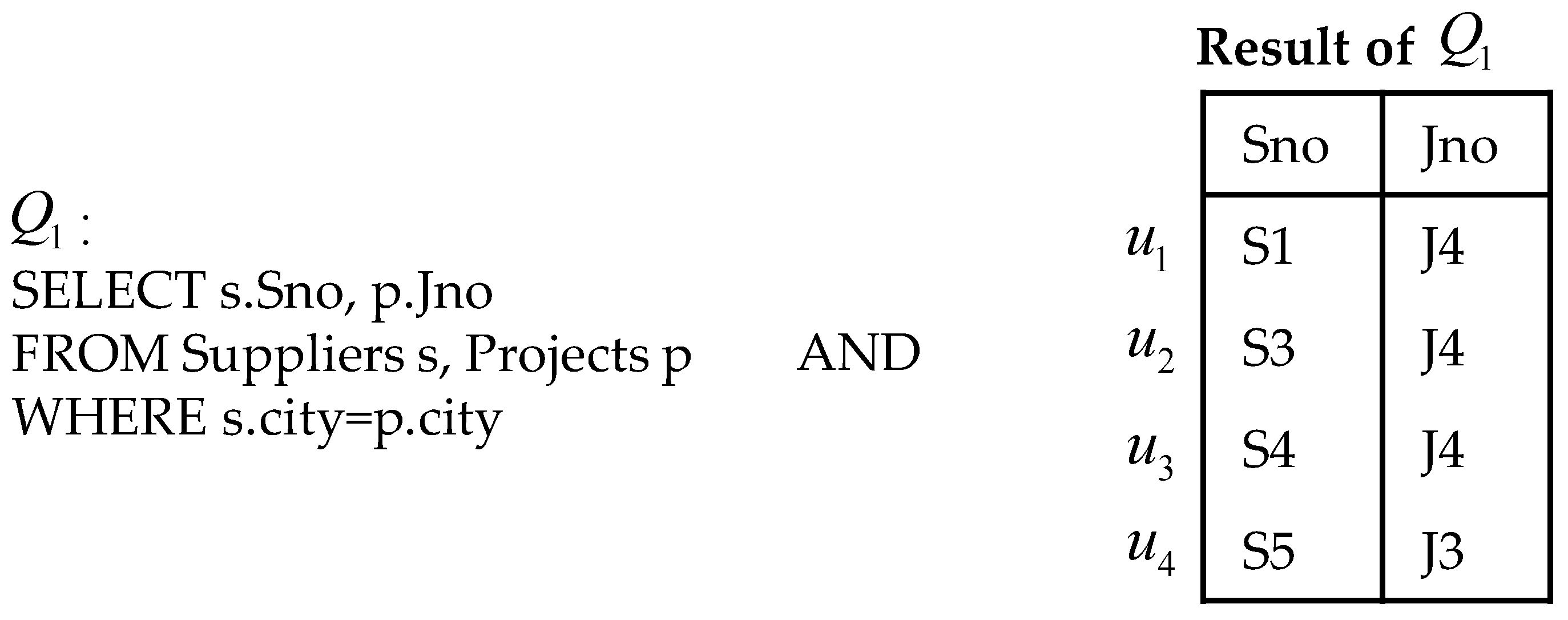
Example 1. 

Consider a query finding all identifier numbers of suppliers and projects located in the same city. As show in Figure 2, $Q_1$ is a typical SQL query, and the corresponding relational algebra is $\prod _{Sno,Jno}(Suppliers S{\infty }_{S.city=P.city }Projects P)$.

According to Definition 1, $u_1\left(\mathrm{S}1,\mathrm{J}4\right)$ has provenance: $Where\left(Q_1,u_1\left[Sno\right]\right)=\left\{s_1\left[Sno\right]\right\}$ and $Where\left(Q_1,u_1\left[Jno\right]\right)=\left\{s_1\left[Jno\right]\right\}$.

Based on where-prov, it is not difficult to extend to tuple granularity. Intuitively, if the complete or partial copy of tuple u is used to compute the output tuple t, then u is the provenance data of t. In other words, when $u\left[B\right]$ is the provenance data of $t\left[A\right]$, then u is the provenance data of t.

Definition 2 (TupWhere). 

Consider a tuple t, its provenance $TupWhere\left(Q,t\right)$ is as follows. $TupWhere\left(Q,t\right)={\displaystyle \cup }\left\{u|u\left[B\right]\in Where\left(Q,t\left[A\right]\right)\right\},\forall A\subseteq Q,B\subseteq A$.

According to Definition 2, the provenance of $u_1\left(\mathrm{S}1,\mathrm{J}4\right)$, $u_2\left(\mathrm{S}3,\mathrm{J}4\right),$ and $u_4\left(\mathrm{S}5,\mathrm{J}3\right)$ in the result of $Q_1$ can be represented as $TupWhere\left(Q_1,u_1\right)=\left\{s_1,j_4\right\}$, $TupWhere\left(Q_1,u_2\right)=\left\{s_3,j_4\right\}$, and $TupWhere\left(Q_1,u_4\right)=\left\{s_5,j_3\right\}$, respectively.

Using where-prov, if a tuple u is fully or partially copied to compute the output tuple t, then u is the provenance data of t. Compared with the value-level where-prov, a schema is at a high level of granularity. Similarly, if tuples of relation table $R_1$ contribute to tuples of relation table $R_2$, we can intuitively infer that the schema U for $R_1$ contributes to the schema T for $R_2$ at the schema level. Consequently, the standardized definitions of field-level and schema-level provenance data can be obtained (Definitions 3 and 4).

Definition 3 (FProv). 

The provenance data of field A: $FProv\left(A\right)={\displaystyle \cup }\left\{B|u\left[B\right]\in Where\left(Q_i,t\left[A\right]\right)\right\}, i=1,2,\dots n,$ where $Q_i$ is any query containing A in the list of target fields.

Definition 3 demonstrates that all fields contributing to the value of every tuple on field $A$ constitute the field-level provenance of field $A$. For example, $FProv\left(Sno\right)=\left\{Supplies.Sno\right\}$.

Definition 4 (SProv). 

The provenance data of schema T: $SProv\left(\mathit{T}\right)={\displaystyle \cup }\left\{{\mathit{R}}_i|u\in TupWhere\left(Q_i,t\right),U\in R_i,u\in U,t\in T\right\}, i=1,2,\dots n,$ where $Q_i$ is any query inserting its querying results to table T.

Under the copy contribution semantics, if tuples of relation table $R_i$ contribute to tuples of relation table $T$ and $u\in TupWhere\left(Q,t\right),t\in T,u\in R_i$, then ${\mathit{R}}_i$ contributes to T at the schema level.

3.4. Representation of Provenance Transformation

In a closed relational database management system that supports data provenance, the process of generating relational data is called provenance transformation. Provenance transformation emerges at different levels of granularity, such as tuples, fields, and values. For the relational data of a given granularity, their provenance transformations form a transformation expression, explaining data creation. To accurately illustrate data provenance, this paper introduces provenance explaining transformation (PET), a method based on transformation expressions. Notably, PET can describe provenance transformation in queries and is exclusive to the provenance transformation of tuples and values.

3.4.1. Tuple and Value Provenance Transformation

Tuples are operating objects in computing the provenance transformation of tuples. Modern DBMS provides a variety of powerful function operations for complex queries. Essentially, such operations can be converted to operations on two-dimensional tables. Our purpose is to eliminate the influence of sophisticated features of query language and, more importantly, to support data provenance for any SQL-like and procedural language with a control structure. Hence, we utilize and standardize five basic operations to construct transformation expressions. We call them meta-transformation, including null transformation (ONull), projection transformation (OProj), group aggregation transformation (OAggr), join transformation (OJoin), and union transformation (OUnion). It is worth noting that these transformations are mainly relational algebraic operations, so it is easy to express SQL-like languages.

Definition 5. 

Copy-based meta-transformations:

• Null transformation $ONull$, $ONull\left(Q\right)=Q$.
• Projection transformation $OProj$, $OProj\left(Q\right)=Q^{\prime },Q^{\prime }\left(I\right)=\left\{t|t=u\left[e\left(A\right)\right], u\in Q\left(I\right), A\in Q\right\}$.
• Group aggregation transformation $OAggr$, $OAggr\left(Q\right)=Q^{\prime }$, $Q^{\prime }\left(I\right)=\left\{t|t=g\oplus aggr\left(G{\left[C\right]}^{*}\right),G\in Q\left(I\right),\forall u\subseteq G,g=e\left(u\left[B\right]\right)\right\}$
• Join transformation $OJoin$, $OJoin\left(Q_1,Q_2\right)=Q^{\prime },Q^{\prime }\left(I\right)=\left\{t|t=u\left[A\right]\oplus v\left[B\right],u\in Q_1\left(I\right),v\in Q_2\left(I\right),A\subseteq Q_1,B\subseteq Q_2\right\}$
• Union transformation $OUion$, $OUoin\left(Q_1,Q_2\right)=Q^{\prime },Q^{\prime }\left(I\right)=Q_1\left(I\right){\displaystyle \cup }{Q}_2\left(I\right)\}$

In the above meta transformations, the Null transformation operation, including the direct copy in Definition 1, filter operations, and other database operations not involving copy transformation do not modify the input tuples, so the input is the output. The projection transformation retains tuples in the specified fields. The group aggregation transformation divides input tuples into groups by specific attribute values, aggregates each group with specified attributes, and outputs the results, where each input group corresponds to an output tuple. The join transformation discovers matched tuples meeting the join condition, and the union transformation merges two input sets into an output. Both join and union operations are binary operations and extendable to multivariate operations. The tuple provenance transformation PET combines the above basic operations to express the provenance transformation process and complex SQL operations in the database. Using the above meta transformations, we define PET as follows.

Definition 6. 

$PET\left(Q,t\right)$, provenance transformation of tuple t:

• $PET\left(\left\{t\right\},t\right)=expr<R>,where\left\{t\right\}\subseteq R$
• $PET\left(ONull\left(Q\right),t\right)=expr<PET\left(Q,t\right)>$
• $PET\left(OProj\left(Q\right),t\right)=expr<OProj\left(PET\left(Q,u\right)\right)>$
• $PET\left(OAggr\left(Q\right),t\right)=expr<OAggr\left(PET\left(Q,u\right)\right)>$
• $PET\left(OJoin\left(Q_1,Q_2\right),t\right)=expr<OJoin\left(PET\left(Q_1,u\right),PET\left(Q_2,v\right)\right)$
• $PET\left(OUnoin\left(Q_1,Q_2\right),t\right)=\{\begin{array}{c}expr<PET\left(Q_1,t\right)> where t\in Q_1\left(I\right)-Q_2\left(I\right)\\ expr<PET\left(Q_2,t\right)> where t\in Q_2\left(I\right)-Q_1\left(I\right)\\ expr<PET\left(Q_1,t\right)> or expr<PET\left(Q_2,t\right)>,else\end{array}$
• $PET\left(OAggr(OUnoin\left(Q_1,Q_2\right)\right),t)=expr<OAggr\left(OUnoin\left(PET\left(Q_1,u\right),PET(Q_2, v\right)\right))>$

In Definition 6, $expr<tf>$ is an expression for the transformation instead of transformation operation $tf$ itself. Take $Q_1$ as an example. For $\forall u\subseteq Q_1$, the provenance transformation of tuple u can be expressed as $OJoin\left(Supplies,Projects\right)$, namely, $Pet\left(Q_1,u\right)=OJoin\left(Supplies,Projects\right)$.

It is worth pointing out that in the above transformations, only the $OAggr$ transformation can aggregate multiple tuples into one tuple. In this case, an output tuple may simultaneously derive from both $Q_1$ and $Q_2$. Therefore, in the process of transforming queries, the output of $OUnoin$ must be used as the input of $OAggr$. Namely, $OUnoin$ must be used as a subexpression in the expression of $OAggr$. Otherwise, $OUnoin$ has no meaning in the transformation expression, and we can replace it with either $expr<Pet\left(Q_1,t\right)>$ or $expr<Pet\left(Q_2,t\right)>$ or both.

Value can be regarded as a tuple with only one field, so the value-level provenance transformation can be derived from the tuple-level provenance transformation. In this paper, we refer to this derivative version as VPET (Value PET). Similar to PET, the expression of VPET is also formed based on meta-transformation. In the context of VPET, the granularity of the data unit is a value rather than a tuple, which is the exact difference between VPET and PET.

Definition 7. 

$VPET\left(Q,t\left[A\right]\right)$. The value provenance transformation of tuple t on field A:

• $VPET\left(\left\{t\right\},t\left[A\right]\right)=expr<A>,A\subseteq \mathit{R}$
• $VPET\left(ONull\left(Q\right),t\left[A\right]\right)=expr<VPET\left(Q,t\left[A\right]\right)>$
• Given $t\left[A\right]=e\left(u\left[B\right]\right),u\subseteq Q\left(I\right)$, we have

  $$VPET\left(OProj\left(Q\right),t\left[A\right]\right)=\{\begin{array}{c}expr<VPET\left(Q,u\left[B\right]\right)>,if expr<e\left(u\left[B\right]\right)>=expr<B>\\ expr<OProj\left(VPET\left(Q,u\left[B\right]\right)\right)>,else\end{array}$$
• Given B and C are group and aggregation fields, $B^{\prime }\subseteq B$, $C^{\prime }\subseteq C$, $\forall u\in G\subseteq Q\left(I\right)$, $g=e\left(u\left[B\right]\right)$, we have

  $$VPET\left(OAggr\left(Q\right),t\left[A\right]\right)=\{\begin{array}{c}expr<OAggr\left(VPET\left(Q,u\left[C^{\prime }\right]\right)\right)>,if t\left[A\right]=aggr\left(G{\left[C^{\prime }\right]}^{*}\right)\\ expr<VPET\left(Q,u\left[B^{\prime }\right]\right)>,if t\left[A\right]=e\left(u\left[B^{\prime }\right]\right), expr<u\left[B^{\prime }\right]>=expr<B^{\prime }>\\ expr<OProj\left(VPET\left(Q,u\left[B^{\prime }\right]\right)\right)>,t\left[A\right]=e\left(u\left[B^{\prime }\right]\right), else\end{array}$$
• Given B and C are group and aggregation fields, $B^{\prime }\subseteq B$, $C^{\prime }\subseteq C$, $\forall s\in G\subseteq Q_1\left(I\right){\displaystyle \cup }{Q}_2\left(I\right),g=\left(s\left[B\right]\right)$, we have

  $$VPET\left(OAggr\left(OUnion\left(Q_1,Q_2\right)\right),t\left[A\right]\right)$$

  $$=\{\begin{array}{c}expr<OAggr\left(VPET\left(OUnion\left(Q_1,Q_2\right),s\left[C^{\prime }\right]\right)\right)>,if t\left[A\right]=aggr\left(G{\left[C^{\prime }\right]}^{*}\right)\\ expr<VPET\left(Q_1,s\left[B^{\prime }\right]\right)>,if t\left[A\right]=e\left(s\left[B^{\prime }\right]\right), s\in Q_1\left(I\right),expr<e\left(s\left[B^{\prime }\right]\right)>=expr<B^{\prime }>\\ expr<OProj\left(VPET\left(Q,s\left[B^{\prime }\right]\right)\right)>,t\left[A\right]=e\left(s\left[B^{\prime }\right]\right),s\in Q_i\left(I\right),i=1,2\end{array}$$
• $VPET\left(OJoin\left(Q_1,Q_2\right),t\left[A\right]\right)=\{\begin{array}{c}expr<VPET\left(Q_1,u\left[B\right]\right)>,t\left[A\right]=u\left[B\right]\\ expr<VPET\left(Q_2,v\left[C\right]\right)>,t\left[A\right]=v\left[C\right]\end{array}$

In Definition 7, for group and aggregation operation $OAggr$, if $t\left[A\right]$ only originates from the group fields, we can infer that the aggregation function contributes nothing to the result. In other words, the transformation of values is not the result of $OAggr$ operation.

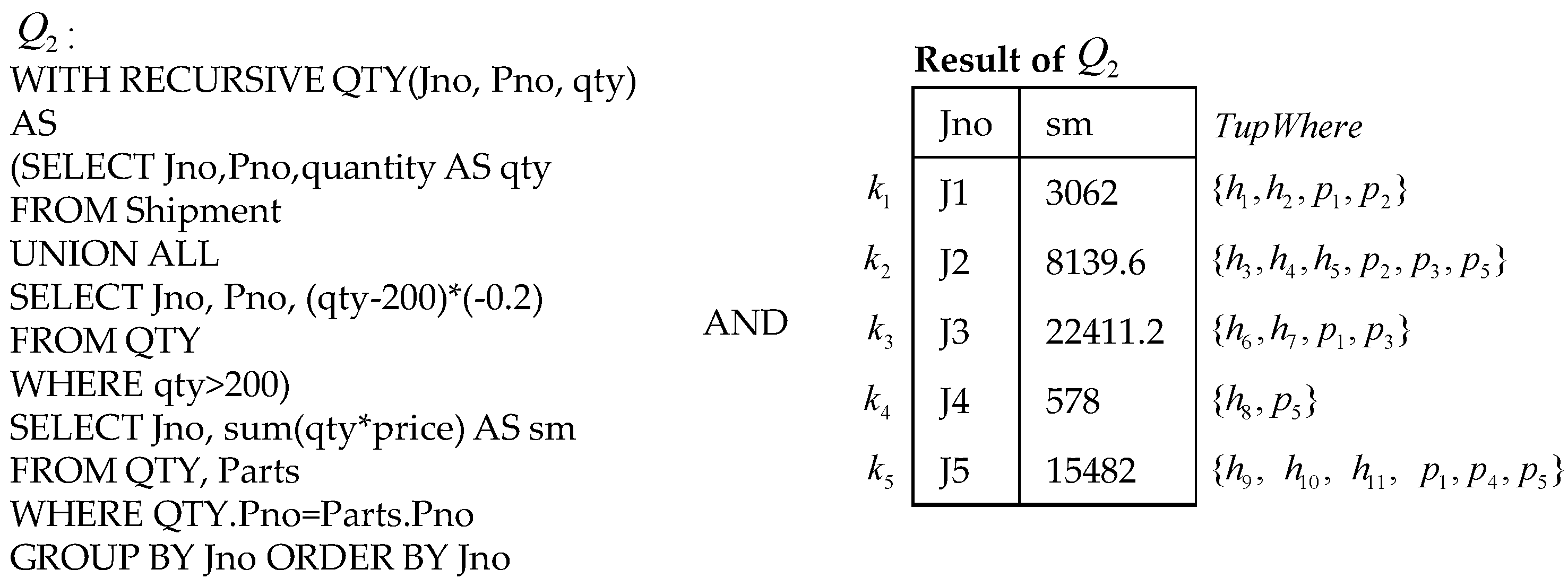
Example 2. 

Consider a query$Q_2$computing the total price after discount for each project (assuming the excess parts can enjoy 20% off when the number of parts exceeds 200).

As shown in Figure 3, the tuple-level where-prov of the tuple k₁ is $\left\{h_1,h_2,p_1,p_2\right\}$. Suppose $Q_2^{\prime }$ is the CTE recursive subquery for $Q_2$. The provenance transformations for all output tuples of $Q_2^{\prime }$ are $OProj\left(Shipment\right)$ and $OProj{\left(OProj\left(Shipment\right)\right)}^{*}$. According to Definitions 6 and 7, the provenance transformation of $k_2$ is $PET\left(Q_2,k_2\right)=OJoin\left(OProj\left(Shipment), OAggr\left(OProj\left(OJoin{\left(OProj\left(Parts\right),OUnion(OProj\left(Shipment\right), OProj(OProj\left(Shipment\right)\right)}^{*}\right)\right)\right)\right))$. The value provenance transformations of $k_2$ on field $Jno$ and $sm$ are $VPET\left(Q_2,\mathrm{J}2\right)=OProj\left(Shipment.Jno\right)$, and $VPET\left(Q_2,8139.6\right)=OAggr\left(OProj\left(OJoin\left(OUnion\left(Shipment.quantity,OProj\left(Shipment.quantity\right)\right), Parts.price\right)\right)\right)$.

3.4.2. Representing Provenance Transformation in SQL with Meta-Transformation

We SQL-revised PET to support full-featured SQL, and we present how PET represents SQLs in this section. For the sake of discussion, assume that the main body of a query is the SQL of ASPJ-CTE-Win-Sub with selection and filter, projection, join, group aggregation, CTE (common table expression), window function, and set operation. Furthermore, PET supports the query language of small features (such as Sort, Limit, and Distinct). For each SQL feature, the representation method based on meta-transformations is described as follows. To illustrate this, we use $subExp{r}_i,i=1,2,\dots ,n$ to represent the transformation expressions that function as the subexpressions of the operations discussed below.

• Ordinary import. Ordinary import is treated as a query on constant relation tables and expressed as $ONull(\perp )$.
• Selection and filter. The filtering operation does not perform any transformation on tuples, so the corresponding transformation expression is $ONull\left(subExpr\right)$.
• Group aggregation, projection, and union are expressed as $OAggr$, $OProj$, and $ONull$, respectively.
• Joins (both input sets contribute to the output) include inner joins, left/right outer joins, and full outer joins. The Cartesian product operation can be treated as an inner join if join conditions always hold. The join transformation is expressed as:
  Inner join: $OJoin\left(subExp{r}_1,subExp{r}_2\right)$;
  Left outer join: $OJoin\left(subExp{r}_1,subExp{r}_2\right)$ or $OJoin\left(subExp{r}_1,\perp \right)$;
  Right outer join: $OJoin\left(subExp{r}_1,subExp{r}_2\right)$ or $OJoin\left(\perp ,subExp{r}_2\right)$;
  Full outer join: $OJoin\left(subExp{r}_1,subExp{r}_2\right)$, $OJoin\left(subExp{r}_1,\perp \right)$ or $OJoin\left(\perp ,subExp{r}_2\right)$.
• Join (when only one of the two input sets contribute to the output). In this case, the other input set plays the role of a filter. Assume that only the left input set contributes, then the join transformation is expressed as $subExp{r}_1$ or $\perp$ (right outer join and full outer join will make the left input set a constant relational table).
• Window function. The window function is an extension of group aggregation in SQL and can be equivalently represented by group aggregation and join. Therefore, the window function is equivalent to $OJoin\left(subExpr,OAggr\left(subExpr\right)\right)$.
• Except operation (Except, $Q_1-Q_2$). The output tuples only come from $Q_1$, so the except operation is expressed as $subExp{r}_1$.
• Intersect operation (Intersect, $Q_1{\displaystyle \cap }{Q}_2$). The output tuples are from $Q_1$ and $Q_2$. In this case, there are two kinds of parallel provenance transformations, denoted as $subExp{r}_1$ and $subExp{r}_2$.
• CTE (Including recursive CTE and non-recursive CTE). Non-recursive CTE can be regarded as a nested subquery. Recursive CTE is divided into a base query and a recursive query on the language structure. The input of the recursive query may be the output of the base query or the output of the previous recursion. The output of the CTE can be regarded as the union of a base query, a recursive query with the base query as the input, and a recursive query with the output of the previous recursion as the input. Therefore, recursive CTE is expressed as $baseExpr$, $recursiveExpr{\left(baseExpr\right)}^{*}$ (the asterisk indicates using the output of the last recursion as the input) or $OUnion\left(baseExpr,recursiveExpr\left(baseExpr\right), recursiveExpr{\left(baseExpr\right)}^{*}\right)$ among the third item that has the premise that the current expression works as a subexpression of the aggregation operation.

Example 3. 

Suppose we have the following query$Q_3$calculating the revenue for suppliers with a window function. The query$Q_3$ and its output are shown in Figure 4.

The first output column derives from the table $Shipment$, and the second column represents an aggregation of each supplier’s revenue on each project. For the above provenance transformation definition, it is easy to see that the PET representation for each tuple can be written as $OJoin\left(OProj(Shipment\right),OAggr\left(OProj\left(OJoin\left(Parts,Shipment\right)\right)\right)$). The value provenance transformations of $q_1$ in field $Sno$ and $revenue$ are $OProj\left(Shipment.Sno\right)$ and $OAggr\left(OProj\left(OJoin\left(Parts.price,Shipment.quantity\right)\right)\right)$.

3.4.3. Representing Provenance Transformation in Stored Procedures with Meta-Transformation

Database-stored procedures are similar to SQL-like languages or other scripting languages, such as Python and Perl. In this paper, we only focus on SQL-like procedural languages, such as T-SQL for SQL Server, PL/SQL for Oracle, and PL/pgSQL for PostgreSQL. The stored procedure covers two kinds of flow structure: data flow (assignment, SQL execution) and control flow (conditional control, loop control). Only the data flow structure addresses the copy transformation relation of the data, while the control flow structure controls the switch branch of transformation. Here, we introduce how to use basic operations to represent each language feature.

• Constant. In procedural language, when statement blocks do not reference any relational table in the database, the data output by this program can be regarded as coming from a constant relational table. Therefore, any query referencing a constant is treated as an ordinary import and expressed as $ONull(\perp )$.
• Assignment. The assignment operation assigns the calculation result of an expression to a variable. If values of an output tuple on some fields come from the variable, then a projection operation is used to project the input variable to the output tuple on these fields. Suppose that $t\left[A\right]=e\left(u\left[B\right]\right),u\in Q\left(I\right),B\subseteq Q$, when A covers all the fields of t, then the transformation expression is $OProj\left(exp{r}_Q\right)$. Otherwise, tuple t must contain values of other field set A′ other than A, and the values are the result of other projection expressions. If there is $t\left[A^{\prime }\right]=e^{\prime }\left(v\left[C\right]\right),v\in Q^{\prime }\left(I\right)$, $C\subseteq Q^{\prime }$, then the transformation expression is $OProj\left(OJoin\left(exp{r}_Q,exp{r}_{Q^{\prime }}\right)\right)$.
• The SQL or dynamic SQL in stored procedures is equivalent to a nested subquery, and we convert it into a subexpression.
• Conditional control statement block. A conditional control structure has multiple switch sub-statement blocks that cannot simultaneously execute, so the tuple can only be from one of the sub-statement blocks. Similar to a union operation, the transformation expressions of conditional control structure are $OUnion\left(subExp{r}_1,subExp{r}_2,\dots ,,subExp{r}_n\right)$ or $subExp{r}_i,i=1,2,\dots ,n$. $OUnion$ is a requisite only when the present transformation is a subexpression of $OAggr$. Therefore, a conditional control operation is equivalent to a union operation.
• Loop control. Assume $t$ is a variable in the body of the loop statement. Before entering the loop statement, $PET\left(Q,t\right)=exp{r}_1$, and the transformation expression of $t$ in the loop body is $exp{r}_2$. After the execution of the loop statement, we have four cases: (a) if the judgment condition of the loop does not meet at the beginning, the loop body statement will not execute the following: $PET\left(Q^{\prime },t\right)=exp{r}_1$; (b) the loop body statement is executed only once as the following: $PET\left(Q^{\prime },t\right)=exp{r}_2$; (c) the loop body statement is executed multiple times, but $exp{r}_2$ does not reference the variable $t$. Therefore, the expression $t=exp{r}_2$ is non-recursive, and the value of $t$ is always the result of the last loop, namely $PET\left(Q^{\prime },t\right)=exp{r}_2$; and (d) the statement of the loop body is executed multiple times, and $exp{r}_2$ is recursive. Then, we have $PET\left(Q^{\prime },t\right)=exp{r}_2{}^{*}$, which shows that loop control is equivalent to one CTE.

Example 4. 

Suppose function$fn\left(x,y\right)$returns the project number and the discount amount, where x and y are inputs representing the discount and the minimum quantity for the discount. The body of this stored procedure is as follows:

03 DECLARE

04 t DISCOUNT; -- DISCOUNT is a custom data type, namely the return type (Jno, amount)

05 r Shipment%rowtype; -- Declare r to be the same type as the tuple of the table Shipment

06 a NUMERIC;

07 p NUMERIC;

08 BEGIN

09 FOR r IN SELECT * FROM Shipment LOOP

10 SELECT price INTO p FROM Parts WHERE Pno = r.Pno;

11 IF r. quantity > x THEN

12 a:= x + (r.quantity − x) *y;

13 SELECT r.Jno, a*p INTO t;

14 ELSE SELECT r.Jno, r.quantity*p INTO t;

15 END IF;

16 RETURN NEXT t;

17 END LOOP;

18 RETURN;

19 END

Assuming the loop in line 9 runs multiple times and the condition in line 11 has been satisfied, the transformation expressions for lines 9 and 10 are $PET\left(Q,p\right)=OProj\left(OJoin\left(Shipment,Parts\right)\right)$. Similarly, the transformation representations of lines 12–14 can be further summarized: $PET\left(Q,a\right)=OProj\left(Shipment\right)$ for line 12, $PET\left(Q,t\right)=OJoin\left(OProj\left(Shipment\right),PET\left(Q,a\right),PET\left(Q,p\right)\right)$ for line 13, and $PET\left(Q,t\right)=OJoin(OProj\left(Shipment),PET\left(Q,p\right)\right)$ for line 14.

4. Representing Data Provenance in DBMS

Where-prov and PET can represent provenance data and transformation in a database. In this section, we propose a relational provenance representation model based on where-prov and PET to comprehensively interpret data provenance from multiple levels (relational schemas, attribute fields, tuples, values), especially the provenance transformation process.

4.1. Schema-Level Provenance Representation

Schema-level data provenance is coarser and more suitable for applications that do not focus on the details. In a transformation-intensive database environment, the relational table instances are the results of relation interactions, which reflect the dependencies between tables at the schema level. Since provenance data between schemas does not have a formal definition, this paper introduces a representation model for schema-level provenance.

Schema-level provenance is a directed graph, G = <V_R, V_O, E>, where V_R represents relation table nodes, V_O denotes the transformation operation nodes, and E is the directed edges set representing the dependencies among V_O, and the dependencies between V_R and V_O. Specifically, we have:

Definition 8. 

(1) Tuple Provenance Graph (TupPGraph), $TupPGraph\left(Q_i,I,t\right)=<V{t}_r,V{t}_o,Et>$ (2) Schema Provenance Graph of T (SPGraph), $SPGraph\left(I,\mathit{T}\right)=<V_r,V_o,E>,where V_r={\displaystyle \cup }V{t}_r,V_o={\displaystyle \cup }V{t}_o,E={\displaystyle \cup }Et,\forall t\in T,TupPGraph\left(Q_i,I,t\right)=<V{t}_r,V{t}_o,Et>$ (3) Schema Provenance Graph of database I (SPGraph),$SPGraph\left(I\right)=<V{I}_r,V{I}_o,EI>,where V{I}_r={\displaystyle \cup }{V}_r,V{I}_o={\displaystyle \cup }{V}_o,EI={\displaystyle \cup }E,\forall \mathit{T}\in \Re$.

From the above definition, the schema provenance graph not only includes the provenance transformation of each tuple but also explains the transformation process between the target relation schema and source relation schema. Similarly, the overall schema provenance graph SPGraph(I) merges all the schema provenance graphs of the database and can explain the specific dependencies between different relation schemas.

Every output tuple has a tuple provenance graph, and multiple output tuples may have the same tuple provenance graph for a query Q, indicating that output tuples can share a tuple provenance graph. Furthermore, two tuple provenance graphs in the same query Q may have the common subgraph, indicating that merging tuple provenance graphs is possible. Therefore, we keep one tuple provenance graph for multiple output tuples and combine different tuple provenance graphs to obtain the schema provenance graph. During the merging process, some nodes may lose information, such as the number of operations or operation objects of the lower nodes. To avoid this, we introduce the “Option’’ node without transformation meaning, which means multiple possible branches for this node.

For example, the tuple provenance graph of transformation expression $PET\left(Q_i,t\right),t\in T$ can be expressed as $G<R^{\prime },O,\eta >$, $R^{\prime }=\left\{R_1,R_2,\dots ,R_m\right\}$,$O=\left\{O{p}_1,O{p}_2,\dots ,O{p}_n\right\}$, where $O{p}_j$ is the $j^{th}$ basic transformation ($O{p}_1$ is the top-level operation), and $\eta$ is a set containing the relations among operations and the relations between operations and reference relation tables.

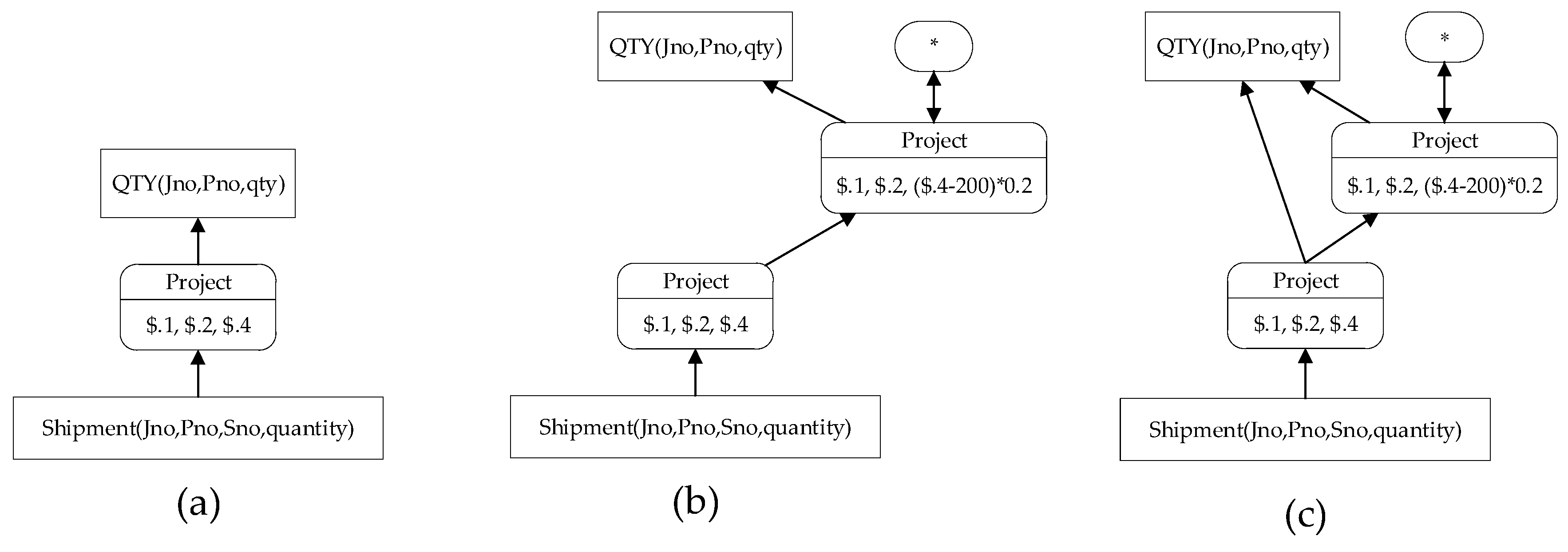
Figure 5 shows the possible tuple provenance graphs of the output tuples of table $QTY$ in query $Q_2$ in Example 2, which is output by the subquery $Q_2^{\prime }$. Figure 5a–c displays tuple provenance subgraphs of the tuple $k_1$ and $k_4$, tuples $k_3$, and tuples $k_2$ and $k_5$, respectively. Notably, the tuple provenance graph in Figure 5c is actually the SPGraph of the query $Q_2^{\prime }$.

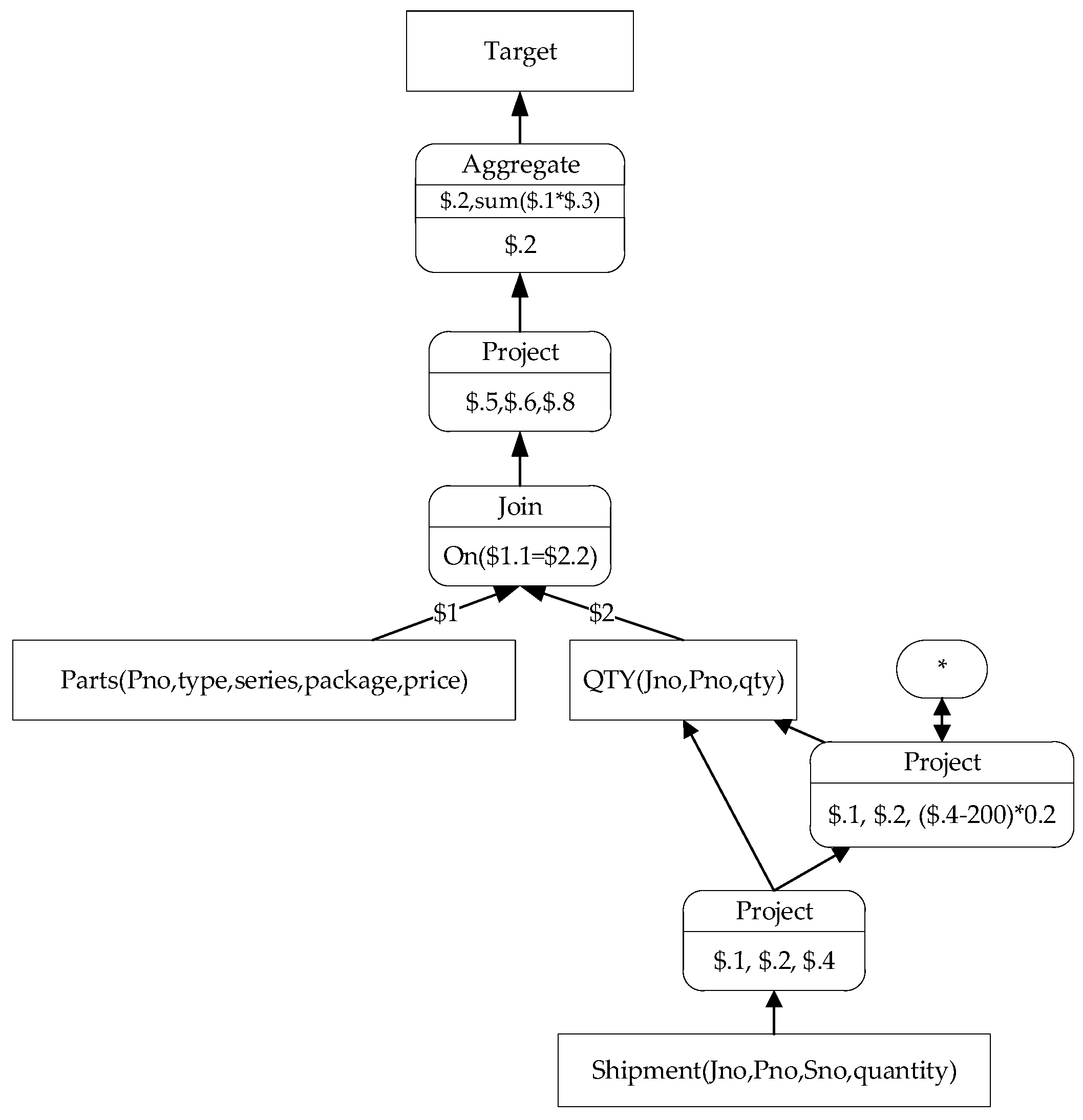
According to the discussion in Example 2, we have $PET\left(Q_2,k\right)=OJoin\left(OProj\left(Shipment\right),OAggr\left(OProj\left(OJoin\left(OProj\left(Parts\right),PET\left({Q_2}^{\prime },k\right)\right)\right)\right)\right)$. It is not difficult to infer that the remaining part of the SPGraph for $Q_2$ is clear and can be merged with the SPGraph for $Q_2^{\prime }$ to obtain the SPGraph for $Q_2$, as shown in Figure 6.

4.2. A Compact Representation of TupPGraph

As a subgraph of schema provenance graph SPGraph, each tuple provenance graph corresponds to one kind of schema transformation relations. To clarify the relationship between TupPGraph and SPGraph and reflect TupPGraph of each tuple in SPGraph (or every possibility in schema transformation relations), we put forward the concept of tuple provenance route (TupPRoute) to represent the provenance of tuples.

Definition 9. 

Tuple Provenance Route(TupPRoute),$TupPRoute\left(Q_i,I,t\right)=<SPGraph\left(I,\mathit{T}\right),BP>$, where$BP=\left\{\right||b_{rid},rid=1,\dots ,MA{X}_{RID}\}$, $b_{rid}=0 if V_{rid}\notin TupGraph$ and$b_{rid}=1 V_{rid}\in TupGraph$.

From the description of the provenance graph, TupPGraph is an expression tree with several branches. Each node in SPGraph has a semantic parent and multiple child nodes in the tree structure. In Definition 9, BP is a bitmap array for the provenance route, and V_rid represents a vertex identified as rid. All nodes in a SPGraph (including relational table nodes and transformation nodes) have an identifier rid that the maximum identifier value is MAX_RID. The rid bit in the BP is set to 1 if a node belongs to a TupPGraph, and otherwise 0. Though rid is theoretically unique, the bitmap may be too large if each node is assigned an identifier bit. Therefore, this paper uses a more compact way to ascertain a route by preorder traversing the schema provenance graph and allocating the same rid for nodes on the same branch, meaning that the value of MAX_RID is small (Algorithm 1).

Algorithm 1.

Alg. generateRids(SPGraph): 01 begin 02 root := SPGraph.rootNode 03 generateRidRecursive(root, 0) 04 end Alg. generateRidRecursive(eachNode, currRid): 05 begin 06 n := eachNode 07 if n.rid has not been assigned then 08 n.rid := currRid 09 end if 10 foreach cn in n.childNodes 11 if count(n.childNodes) = 1 then 12 generateRidRecursive(cn, currRid) 13 else 14 generateRidRecursive(cn, currRid + 1) 15 end if 16 end foreach 17 end

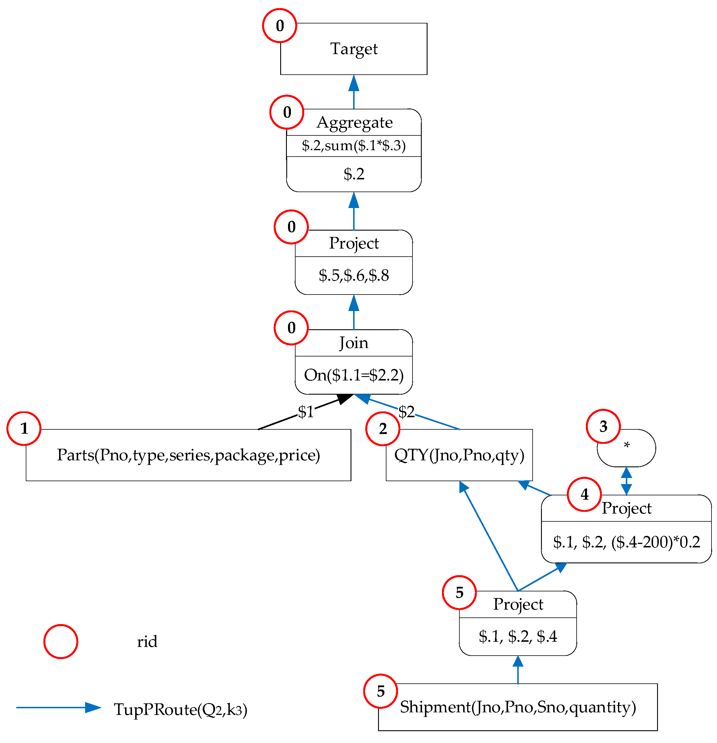
Figure 7 shows the bitmaps corresponding to the three provenance routes in the query Q₂ (base query, recursive query with base query as input, recursive query with the last recursion as input) are “101001”, “101111”, and “110000”. Combining the bitmap array and the schema provenance graph, we can deduce the transformation path of the tuple $k_3$ in the provenance graph (the blue path in the figure).

4.3. Field and Value Level Provenance Representation

Value provenance transformation (VPET) derives from the provenance transformation of tuples. Using a similar way of representing schema provenance graph and tuple provenance route, we utilize the field provenance graph (PGraph of Field, FPGraph) and value provenance route (VPRoute) to represent field- and value-level provenance. For $VPet\left(Q_i,I,t\left[\mathit{A}\right]\right)$:

Definition 10. 

(1) PGraph of Value (VPGraph), value provenance graph  $VPGraph\left(Q_i,I,t\left[\mathit{A}\right]\right)=<$ $V{v}_r,V{v}_o,Ev>$ (2) PGraph of Field (FPGraph), provenance graph for field A, $FPGRaph\left(I,\mathit{A}\right)=<V_r,V_o,E>,where, V_r={\displaystyle \cup }V{v}_r,E={\displaystyle \cup }Ev,\forall t\in T VPGraph\left(Q_i,I,t\left[\mathit{A}\right]\right)=<V{v}_r,V{v}_o,Ev>$. (3) PRoute of Value (VPRoute), value provenance route $VPRout\left(Q_i,I,t\left[\mathit{A}\right]\right)=<FPGraph\left(I,\mathit{A}\right), BP>, BP=\left\{\right||b_{rid},rid=1,\dots ,MA{X}_{RID}\},b_{rid}=0 if V_{rid}\notin TupGraph\left(Q_i,I,t\left[\mathit{A}\right]\right),b_{rid}=1 if V_{rid}\in TupGraph\left(Q_i,I,t\left[\mathit{A}\right]\right)$.

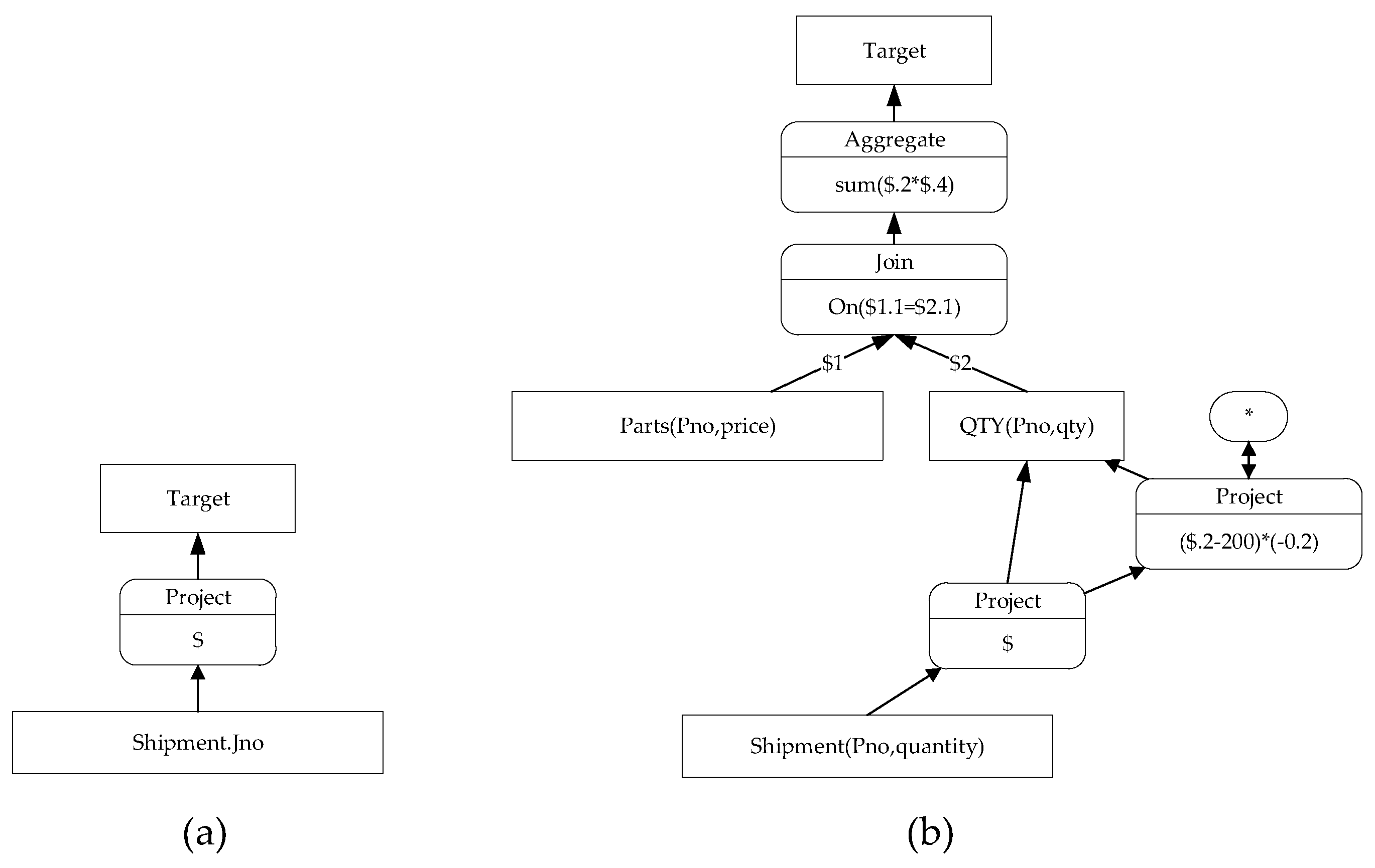
Looking back to Example 2 in Figure 3, the VPET representation for each record in field $Jno$ is $OProj\left(Shipment.Jn\right)$. It is easy to represent the provenance graph for field $Jno$ (Figure 8a). For field $sm$, the provenance transformation representations corresponding to each tuple are $OAggr\left(OJoin\left(Ounion\left(Shipment.quantity, OProj\left(Shipment.quantity\right)\right), Parts.price\right)\right)$ and $OAggr\left(OJoin\left(Shipment.quantity, Parts.price\right)\right)$, as shown in Figure 8b.

4.4. Implementation of Data Provenance in PostgreSQL

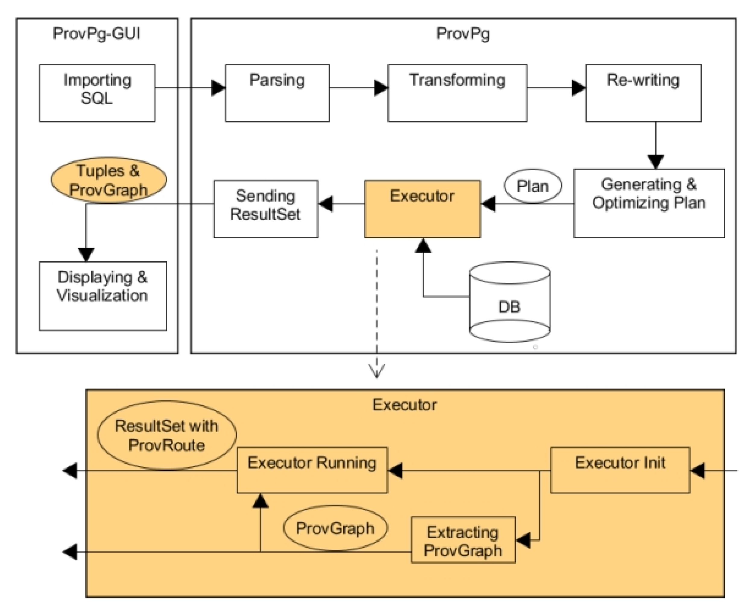
We implemented the model of provenance graph and provenance route in PostgreSQL and provided a client to query and visualized the provenance information. We refer to this improved system as ProvPg. ProvPg has a graphical client known as ProvPg-GUI.

The primary function modules added in ProvPg include the extraction and query of provenance information. The provenance information extraction is implemented by the provenance extraction subsystem. In addition, ProvPg provides a series of query interfaces in the client to support provenance information query and visualization.

ProvPg (Figure 9) is accomplished by using the Hook mechanism of PostgreSQL to add extended functions, and the source code of the Executor is modified. For the plan tree of a query, the processing flow is: (a) Before executing the query, a schema provenance graph (SPGraph) is extracted and produced with the help of the structural information of the plan tree. (b) During the execution of the plan tree, each time a tuple is an output, the corresponding provenance route (TupPRoute) is extracted in the form of a bitmap array. The bitmap array will be inserted into the output tuple as an additional field value. Finally, the client will receive two result sets. One is the output tuple set (with the provenance route), and the other is a provenance graph in the format of JSON. The graphical client ProvPg-GUI is used to receive the SQL input by the user, display the returned query results, and visualize the provenance graph and provenance route.

In order to evaluate the impact of ProvPg on PostgreSQL’s query engine, we conduct TEC Benchmark™ H [47] (TPC-H) test on ProvPg and PostgreSQL. The computation overload of ProvPg on PostgreSQL is analyzed. Our TPC-H instance contains eight relational tables, and we test 22 customized pieces of SQL on this instance (Standard SQL 92). Although the 22 SQLs are missing some features, such as CTE, and are not involved in the stored procedure, the performance of the query engine mainly depends on underlying physical operations, such as tuple scanning, join, and sort. The 22 SQLs have covered the primary calculation process of the query engine. The major significant load of stored procedure in PostgreSQL lies in the execution of a query plan. Therefore, the TPC-H criterion is sufficient to compare ProvPg with the original PostgreSQL.

We construct three datasets ranging from 1G to 4G and 10G for the query tests. The specific running environment is (a) CPU: 64-bit, Intel(R)Core (TM) i5-4460 3.20 GHz; (b) memory: 12G; (c) operating system: Ubuntu 12.04 for operating system; (d) kernel: Linux 3.5.0; (e) PostgreSQL: version 9.5.0. Table S1 shows the query execution time of PostgreSQL and ProvPg on the above dataset. Figure S1 shows the ratios of overhead imposed by the data provenance module. The experiment results indicate the following:

The overall extra cost is relatively small and within acceptable limits. The experiments show that, except for Q2, Q10, Q13, and Q18, the extra cost resulting from the provenance module for each SQL is less than 5%, and the average overhead for three kinds of load sizes is all below 3%. Taking the benefits from data provenance into consideration, we believe that the additional cost is acceptable.

There is no positive correlation between the extra cost and load size. For different-sized datasets, the extra cost of ProvPg on PostgreSQL is stable overall and does not dramatically fluctuate according to data scale. Therefore, we think the extra cost of a query is predictable and estimated.

We also analyze the correlation between the extra cost ratio and execution strategy of the database engine. The Pearson’s correlation coefficient of R₁ and R₂ demonstrate that the extra cost ratio is related to the materialization ratio when we increase the load (Tables S1 and S2), and the dataset scale is more than 10G. The correlation is more significant when we exclude Q8 and Q9 from the SQLs, indicating that materialization clearly prolongs the running time of the extended system. Furthermore, the underlying operation of the database system also affects the increment of the overhead. For example, as Q8 and Q9 mainly perform hash operations, the overhead caused by the provenance module is low even when their materialization ratios are high. As a contrast, Q18 needs to execute a sort operation, and the overhead ratio is high even if it has a small materialization ratio on 1G, 4G scale.

5. Conclusions and Future Work

The lack of support for full-featured SQL and procedural query languages in relational databases and, in particular, the absence of consideration for provenance transformation have seriously limited the application of data provenance. This paper proposes a provenance model and explains the application of our model in actual scenarios to resolve the above limitations. Firstly, we presented a provenance representation PET-based method on where-prov and further introduced the notion of a provenance graph and provenance route. Then, we described the provenance transformation process from relational tables, fields, tuples, and values, which are helpful for understanding and analyzing the dependence and transformation relationship between data. Furthermore, the provenance model is significant for implementing a fully automated debugging and elimination system or tool.

We also implemented our model and extended PostgreSQL to ProvPg with new features, such as database provenance information query and visualization. The implementation of ProvPg verifies the feasibility of applying our model and method and provides new implementation ideas and solutions for capturing provenance information in full-featured SQL and procedural languages. We are confident that our provenance model could be applied to specific business scenarios and make targeted optimizations in subsequent research, such as data debugging and exclusion.