Abstract
Multi-cell cooperative control can be competent for the current increasingly complex biomedical experiments, greatly improving the efficiency of cell manipulation experiments. At present, this kind of multi-cell cooperative control algorithm is becoming more and more important. In this study, holographic optical tweezers are used to capture multiple cells, and a cell manipulation controller is designed based on the Fuzzy Brain Emotional Learning (FBEL) neural network. Firstly, the dynamic model of trapping yeast cells by optical tweezers is analyzed. The distance between the trap position and the cell position is constrained to avoid cell detachment due to the trap moving too fast. Then, the design cell manipulation controller is relied upon to realize single transport trajectory tracking control. Finally, a multi-cell cooperative control algorithm is designed, and combined with the cell manipulation controller, a multi-cell cooperative controller based on the FBEL neural network is formed. The error between the cell position and the desired trajectory is the input of the multi-cell cooperative controller. The output of the multi-cell cooperative controller is the optical trap position, which is used to realize the cooperative control of multiple cells by holographic optical tweezers. The simulation results showed that the multi-cell cooperative controller based on the FBEL neural network can effectively control multiple yeast cells and quickly converge the cell formation, while ensuring a higher control accuracy than other traditional cell manipulation controllers. It provides a new solution for the efficient and precise automatic manipulation of multiple cells.
1. Introduction
In 1986, Ashkin et al. successfully used electrolyte particles trapped by a single-beam laser focused with a high numerical aperture [1], and the optical tweezers technology was born. Optical tweezers use the mechanical effect of momentum transfer between light and particles to manipulate microscopic objects. This indirect manipulation can avoid the energy generated during manipulation from destroying or changing the structural characteristics of the target. Therefore, optical tweezers technology has been favored by many scholars. Especially in the field of biomedicine, due to the non-contact characteristics of optical tweezers, which can avoid damage to cells during manipulation to the greatest extent, they are indispensable in research experiments such as cell sorting [2], cell fusion [3], and cell transport [4]. The technical support of optical tweezers has been widely used.
At present, many scholars have used optical tweezers to conduct complex longitudinal studies on single cells [5,6,7]. Researchers’ needs for biomedicine have tended to be more efficient and complex multicellular manipulation, such as coordinating multicellular acceleration of wound healing [8], or pulling multicellular unblocked blood vessels [9]. Such experiments can often show much greater application value than single-cell manipulation in practice. During the development of optical tweezers, various optical tweezers tools emerged [10,11,12,13,14]. Among them, holographic optical tweezers can simultaneously generate multiple optical traps [15], so that multiple cells can be captured and manipulated. This technique for generating multiple optical traps offers the possibility to efficiently manipulate and control multiple cells [16]. However, most of the previous studies on cells focused on the analysis of biological characteristics and application purposes of various cell experiments, while ignoring the process of manipulating cells. Most of the existing cell manipulation controls are manual, and the operation is complex, time-consuming, and unreliable in accuracy. Some scholars have used PI control and PID control [17,18]. Simple feedback control strategies are also used for the manipulation and control of moving particles [19]. These methods have relatively low control precision for cells. While achieving high efficiency, multicellular manipulation should also satisfy high-precision control. Therefore, the high-precision automatic operation of cells has become one of the key breakthroughs in optical cell manipulation.
With the research of neural network theory and application, more and more neural networks are used in various control systems, including back propagation (BP) neural network [20], Radial Basis Function (RBF) neural network [21], and other networks [22,23,24,25], which effectively improves the control performance and has been verified in many studies. Among many neural networks, the neural network of the brain emotion learning model uniquely simulates the human brain mechanism, mathematically simulates the emotional activities of the amygdala and related parts of the brain, and can improve the efficiency of the neural network controller [26]. On the other hand, using fuzzy theory can better generalize uncertain data in reality [27,28,29]. The fuzzy reasoning system is introduced into the neural network of the brain emotion learning model to form the FBEL neural network. Compared with other traditional neural networks, the FBEL neural network makes full use of prior knowledge in the fuzzy control and expresses knowledge with a small number of fuzzy rules. The received external data information can be learned more effectively, the fitting ability of nonlinear functions is enhanced, and the learning ability of the network is improved. Therefore, it has been widely used in various application domains, such as classification, signal processing, nonlinear system approximation, etc. [30,31,32]. Due to its excellent nonlinear function approximation ability, applying it to cell manipulation will effectively improve the manipulation accuracy of experiments.
In view of the low efficiency of manual manipulation in the current cell manipulation, there is an application limitation of single-cell manipulation and an inability of cell control precision to meet the increasing demand for high-precision cell manipulation. This paper aims to study a new efficient and accurate cooperative control method for cell manipulation in a holographic optical tweezers system, in order to improve the manipulation efficiency and control precision of single cells and multi-cells. Holographic optical tweezers have the advantage of creating multiple optical traps to simultaneously capture cells and avoid contact damage. In this paper, the dynamic model of the cells captured by the optical trap generated by holographic optical tweezers is firstly established, and the constraints on the distance between the optical trap and the cells are added to prevent the abnormal damage of the cells caused by the high-speed movement of the optical trap, ensuring the control cells can be stably captured by the optical trap. Secondly, a FBEL neural network-based cell manipulation controller for holographic optical tweezers is designed and proposed, and the Lyapunov theory is used to verify the convergence of the controller’s core FBEL neural network. In order to realize the coordinated movement of multi-cells, the multi-cell dynamics model is extended. A virtual reference point and the corresponding virtual cells at the reference point are added to the multi-cell, and a matrix of expected spacing of each cell is introduced. By designing the multi-cell cooperative control algorithm and combining the cell manipulation controller, a multi-cell cooperative controller is proposed to realize the multi-cell cooperative control. Finally, take yeast cells as an example. Through simulation experiments, it is confirmed that the cell cooperative controller based on the FBEL neural network can successfully realize the control of a single yeast cell and the cooperative control of multiple yeast cells. Compared with other traditional cell manipulation controllers and other neural networks as controllers, the proposed FBEL neural network cooperative controller has smaller evaluation index values and better control performance. It provides strong technical support for the high-precision automatic manipulation of cells in modern biomedical engineering.
The rest of this paper is organized as follows: Section 2 discusses the principle of the optical tweezers system and the dynamic model of holographic optical tweezers to manipulate cell motion. Section 3 is the design of the cell manipulation controller, including the network structure and convergence analysis of the FBEL neural network. Section 4 describes the multicellular dynamics model and the design method of the cooperative controller. Section 5 is the simulation experiment verification. Section 6 is the conclusion.
2. Cell Manipulation Based on Holographic Optical Tweezers
2.1. Principle of Optical Tweezers Technology
Optical tweezers use a highly concentrated laser beam to exert a force on a particle to trap and manipulate it. The transmission of momentum is accompanied by the propagation of light. According to geometrical optics, the light will be refracted and reflected through a particle when its refractive index is greater than that of its surroundings. The refraction of light on the particle creates a pull on the particle, a gradient force. The reflection of light exerts a scattering force on the particle, which is directed in the direction of light propagation. As shown in Figure 1, two rays a and b are uniform, so the resultant direction of the gradient force Fa and Fb points to the beam focus. The resultant force stabilizes the particle at the focal attachment, where the force on the particle is balanced. The particles are stably trapped in the center of the light trap. If the intensity of the light field is even when the intensity of light b is higher than that of light line a, the force Fb is greater than that of Fa. Thus, the particle is pushed to the side with the lower force until the particle returns to the equilibrium point, where the field intensity of light a is equal to that of light b. The particles are stably trapped in the center of the optical trap.
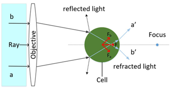
Figure 1.
Schematic diagram of optical tweezers capturing particles.
2.2. Holographic Optical Tweezer System
Holographic optical tweezers load the hologram onto the SLM (Space Light Modulator) to modulate the phase. The laser’s single incident light is divided into numerous separate beams by SLM, which is utilized to generate any type of light field. The process of catching, controlling, and transferring the cells is then accomplished by creating many optical traps through the microscopic objective lens. Image processing determines each cell’s location beneath the microscope and sends that information to the camera for imaging [33].
2.3. Dynamic Model
Yeast cells are captured by light pinching in the culture environment and are mainly subjected to five forces: optical force, viscous resistance, buoyancy, gravity, and Langevin force. The object of this paper is on the x-y plane. Capture cells move in the x-y plane. The forces in the z-axis direction, including the optical force, buoyancy, and gravity in the z-axis direction, are balanced. The force on the z-axis does not affect the x-y plane, so it can be ignored [34]. In the process of cell transportation, the Langevin force can also be ignored because the Brownian motion caused by the Langevin force is relatively small [35,36,37].
The cells captured by optical tweezers are mainly affected by the optical trapping force and viscous resistance [38,39]. The expression is:
where represents cell mass, represents cell position, Ft represents the optical trapping force, and Fd represents drag force.
In this paper, yeast cells were taken as the control object, and their diameters were generally about 5 μm to 6 μm. The captured cell velocity is not more than 15 μm/s. Therefore, the maximum Reynolds number . In a fluid environment with a low Reynolds number, the inertial force on the object can be neglected [38,40,41,42]. Equation (1) can be expressed as follows:
In general, the wavelength of the laser for optical tweezers is smaller than the diameter of the cell. In this case, the value of the optical trapping force can be calculated by the ray optical model:
where represents the optical trap stiffness. represents the position of the optical trap center. represents the distance between the optical trap center and the cell center. r0 represents the distance between the optical trap center and the cell center when the optical trap force Ft reaches its maximum.
The optical trap stiffness is usually a positive constant number. The magnitude of the optical trapping force Ft is related to the distance from the center of the optical trap to the center of the cell. The distance between the center of the optical trap and the center of the captured cell is zero when the optical trap is at rest, and the force of the optical trap acting on the captured cell is also zero. The distance from the center of the optical trap to the center of the cell increases with the change of the position of the optical trap, so the optical trap force also increases. The optical trapping force reaches the maximum value when the distance between the two is r0. When the distance between the centers of the optical trap and the cell is greater than r0, the magnitude of the optical trap force decreases with the increase of the distance. When the optical trap force decreases to zero, the cell will escape from the trap. In conclusion, ensuring that the cell will not escape from the control of holographic optical tweezers is important. Therefore, it is necessary to restrict the distance between the centers of the optical trap and the cell. The general practice is to limit the distance between the two to r0. In particular, it should be noted that the value of r0 is related to the radius r of the captured cell. For the captured cells with different radii, the corresponding r0 values can be determined when they are trapped by the optical trap and the optical trap force reaches the maximum value [43]. Figure 2 showed the relationship between the optical trap force and for cells with different radii, where i = 1, 2, 3, 4, 5. The cell with a larger radius will have a larger value of r0. According to the ratio of r0 to the cell radius r, the value of r0 can be roughly obtained. This practice will cause a small deviation in the value of r0. However, because the slight deviation from r0 will only change the magnitude of the optical trap force slightly, it will not cause the cell to escape. Therefore, the system remains stable.
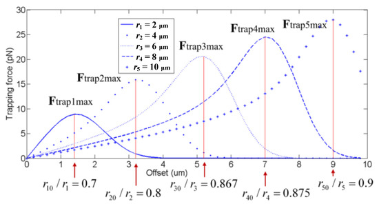
Figure 2.
The relation between the optical trap force and [43].
The viscous resistance can be calculated by Stokes’ formula [44]:
where represents the viscosity of the mucus and represents the radius of the trapped cell.
It is very important to ensure that cells do not escape the control of holographic optical tweezers. Therefore, it is necessary to constrain the spatial position of cells and optical traps. The general practice is to limit the distance between them to r0. The constraint is .
According to (2)–(4), and the constraints, the dynamic model of cell movement manipulated by holographic optical tweezers can be obtained:
where represents the viscous resistance coefficient. represents the distance between the optical trap center and the cell center. r0. represents the distance between the optical trap center and the cell center when the optical trap force Ft reaches its maximum.
3. Single-Cell Manipulation Control
3.1. Dynamic Model Analysis
Since there is a certain distance between the center of the optical trap and the cell center, the cell may overflow during the operation of holographic optical tweezers, so the distance between the center of the optical trap and the cell center should be limited to a certain range r0. In this paper, the position of the center of the optical trap and the center of the cell is described by the two-dimensional plane coordinate system, and the X and Y direction parameters are limited. Therefore, can be disassembled and expressed as:
where , represents the position of the cell center in the X direction; represents the position of the cell center in the Y direction. C , represents the position of the optical trap center in the X direction; represents the position of the optical trap center in the Y direction;
Substituting (6) into (5), the following can be obtained:
where is the environmental coefficient of the cell solution. The value of holographic optical tweezers operating yeast cells at different speeds is shown in Table 1:

Table 1.
Values of β/k in yeast cells [45].
3.2. Cell Manipulation Controller Design
Changing the trapping force of the cell with holographic optical tweezers is a typical way to alter cell motility. The position of the optical trap center produced by the holographic optical tweezers directly affects the trapping force. Therefore, by altering the center point of each optical trap, the direction of the related cell’s movement may be regulated. The holographic optical tweezers can acquire the real-time position of the cell in the altered environment depending on the image processing technology, which is advantageous for better control of the cell.
In order to accurately output the position of the optical trap and improve the control accuracy of cell manipulation, a neural network is used as the main controller. The FBEL neural network consists of two systems: the first system is the amygdala, which is similar to the mammalian brain and is involved in emotional judgment. The second system is the orbitofrontal cortex, which controls emotions. This neural network has strong learning ability and fast convergence speed, and can effectively approximate any nonlinear system [30,31,32].
The type-1fuzzy logic systems can be used to achieve the fuzzy inference of the proposed FBEL neural network with the center average defuzzifier, product interface rule, singleton fuzzifier, and Gaussian membership function given by IF–THEN fuzzy rules [46]. Considering the two systems of the FBEL neural network model, the fuzzy inference systems of the proposed FBEL neural network also consists of two fuzzy rule bases.
One is the amygdala fuzzy system:
If I1 is G1m and I2 is G2m, …, IN is GNm, then A = Dnm
The other is the orbitofrontal cortex fuzzy system:
(for n = 1, 2, …, N, m = 1, 2, …, M), where N is the input dimension, is the fuzzy set for the nth input and mth is the amygdala weight for the output corresponding to the nth input, and the th layer in the consequent space, and A is the output of the amygdala; is the orbitofrontal cortex weight for the output corresponding to the nth input and the th layer in the consequent space, and O is the output of the orbitofrontal cortex.
If I1 is G1m and I2 is G2m, …, IN is GNm, then O = Bnm
The structure of the FBEL neural network is shown in Figure 3. It can be roughly divided into five layers. The first layer is the input layer. The second layer is the sensory cortex. The third layer is the weight space layer. The fourth layer is the amygdala and orbitofrontal cortex. The fifth layer is the output layer.
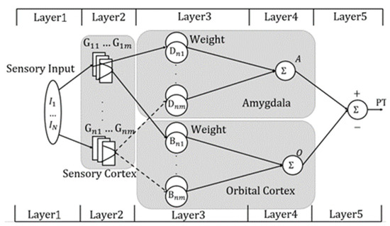
Figure 3.
Structure of the FBEL neural network model.
(1) First layer
This layer is the data input layer.
(2) Second layer
Each neuron uses the input signal to activate the sensory cortex for fuzzy reasoning, and the membership function is a Gaussian function with better universality [46,47]:
where m represents the mth neuron, εnm and represent the mean and variance of the Gaussian function, respectively.
(3) Third layer
holds the weight space of the amygdala and receives the output of fuzzy inference rules from the sensory cortex. holds the weight space of the orbitofrontal page cortex and also receives the output of fuzzy inference rules from the sensory cortex.
(4) Fourth layer
The emotional weight is combined algebraically with the output of fuzzy inference rules in the sensory cortex, and this process is defuzzification. Part of that is amygdala output:
Similarly, the other part is the output of the orbitofrontal cortex:
(5) Fifth layer
It is the final output of the FBEL neural network, produced by the combined action of the amygdala and orbitofrontal cortex.
where U represents the output of FBEL neural network, and A and O represent the output of the amygdala and the orbitofrontal cortex, respectively.
In this paper, the FBEL neural network is used as a controller to control the movement of cells on the set desired trajectory. Define the relative error between the actual cell position and the ideal desired trajectory :
where e is the error between the model output and the expected output and X represent the expected position of the cell and the position of the cell, respectively.
The initial output of the FBEL neural network is not on the predetermined trajectory of the cell. This is because the neural network does not approximate the nonlinear system, and the parameters , , , and do not reach the ideal weight. The weights of amygdala and orbitofrontal cortex are adjusted by reward signals and learning rules.
Next, the update of network parameters will be described in detail. The reward signal is defined as a function of the error signal and the model output:
where and are the weight coefficients that affect network error e and network output U.
The difference between reward signal S and amygdala output A determines the update . Similarly, parameter updates in the orbitofrontal cortex are dominated by both network output U and reward signals S.
where and are the learning rates of the amygdala and orbitofrontal cortex, respectively, and is the fuzzy set after the network input is fuzzified.
The mean and variance of the Gaussian function of the FBEL neural network are updated by the gradient descent method. The loss function E is defined as:
The mean adaptive process of Gaussian function can be expressed as:
The variance adaptation process of Gaussian function is expressed as:
where and represent the learning rate of the mean and variance of the Gaussian function, respectively.
The final parameter updating law of the weight adaptive learning algorithm of the FBEL neural network controller is:
The trajectory-tracking control of the cell manipulation is realized by the FBEL neural network controller. Figure 4 shows the structure diagram of the closed-loop adaptive controller based on the FBEL neural network.
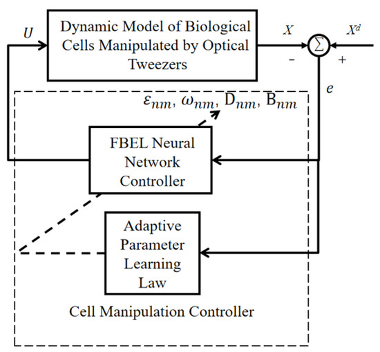
Figure 4.
Structure diagram of a closed-loop system based on the FBEL neural network.
In the cell manipulation controller, the error e between the desired trajectory and the actual position of the cell X is taken as the input of the FBEL neural network controller, and the output of the FBEL network is taken as the output of the adaptive controller, which is the position of the optical trap center in this paper. Substituting the output position of the optical trap into Equation (5), the position of the cell controlled by the optical trap generated by the holographic optical tweezers can be calculated, and finally, precise cell manipulation can be realized.
3.3. Convergence Analyses
In the above adaptive learning algorithm of neural networks, (20) and (21) adopt the gradient descent method to learn and optimize their parameters. The FBEL neural network is iterated several times, and the model parameters are estimated by the loss function at each step. The learning rate is the progress controlling the model learning in the iterative process, which determines whether the objective function can converge and when it converges to the minimum value. If the learning rate is too large, the step length of each learning will be long. Gradients may oscillate around the minimum or fail to converge. When the learning rate is too small, convergence is slow. It is very likely to enter a local minimum and fail to reach a better solution.
Suitable learning rates and are therefore found by the Lyapunov stability theorem to ensure stable convergence of the system in order to achieve the fastest convergence and optimal solution. It is worth mentioning that the convergence analysis is the analysis of the FBEL neural network under the system model. Not only for single-cell control, but also for multicellular control.
The Lyapunov function P is chosen as:
Then the change is as follows:
The prediction error can be expressed as:
where represents the change of .
In (28), can be obtained from (20)
Substituting (20) and (29) into (28), we can obtain:
Therefore, the change in the Lyapunov function is:
According to (31), when , and . So the system is stable and convergent.
Similarly, it can be proved in this way. When , the system is stable and convergent.
4. Multiple Cell Manipulation Control
4.1. Multi-Cell Dynamics Model
In this paper, biological cells are used as control objects. Target cells are separated from other cells according to specific needs, and target cells are transferred to specific areas. This approach has significant drawbacks, poor economy, and low efficiency when used on a single cell. In this study, the cost may be somewhat decreased and the efficiency can be raised by simultaneously regulating several target cells in the target area. The dynamic model of multicellular control was established as follows:
where represents the viscosity resistance coefficient, represents the stiffness of the optical trap, Ci represents the position of the optical trap, Xi represents the actual position of the ith cell, represents the distance between the center of the ith cell and the center of the optical trap, and represents the distance between the center of the ith cell and the center of the optical trap when the optical trap force Ft reaches its maximum value.
4.2. Multi-Cell Controller Design
There is a chance that cells could collide when holographic optical tweezers are in action. The control model’s effectiveness is significantly diminished in the event of a collision. As a result, it is important to keep the space between each cell reasonable. In this study, the problem of cell formation is transformed into a problem of tracking ideal trajectories by adjusting each captured cell to maintain a reasonable distance from other cells. It is necessary to establish a virtual location as the origin of reference for the multicellularity. Since each cell maintains a specific positional relationship with the virtual position, the position information of the reference position can be used to create a cell formation, as shown in Figure 5:
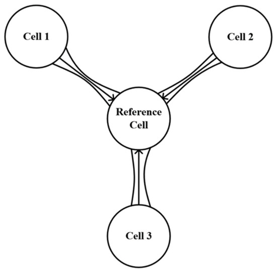
Figure 5.
Reference diagram of multicellular formation position.
In this paper, it is assumed that there is a virtual cell with a reference origin and its position can be expressed as XR. The virtual cell moves in strict accordance with the set ideal trajectory. During the uniform movement of the formation, other captured cells need to keep a certain distance from the virtual cells. Therefore, the χ formation matrix is introduced to effectively control the movement of the formation.
where χ represents the expected distance between each captured cell and the virtual cell, which can be obtained by setting the ideal formation matrix.
According to (33), the error between the actual position of each cell and the expected formation trajectory in multi-cell manipulation can be obtained:
where is the error vector of each captured cell.
The structure of the multicellular cooperative controller based on the FBEL neural network is shown in Figure 6.
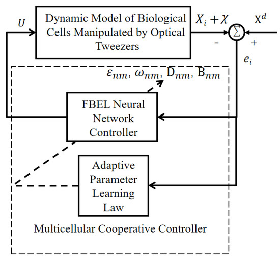
Figure 6.
The structure of the multicellular cooperative controller based on the FBEL neural network.
By changing the control input of the cell manipulation controller in Figure 4 to the multi-cell error redesigned in this section, a new multi-cell cooperative controller is constructed. At this time, the output U by the controller is the position of the optical trap that can manipulate each cell to the desired trajectory.
5. Simulation Results
5.1. Control Single Cell
In this section, the superiority of the FBEL neural network-based cell manipulation controller proposed in this paper is verified by MATLAB experiments when using holographic optical tweezers.
In practice, the environment in which cells live is complex and changeable. Additionally, the cell cannot move in a straight line. Although point-to-point linear control is easy to implement, it is necessary to avoid cell collision to ensure cell safety. Some researchers use circular trajectories to control cell movement. This mode of transportation is too limited [45]. The trajectory tracking control method is used to set the desired trajectory in advance to control cell transport. In this way, the collision between cells and obstacles in the process of moving can be effectively avoided [38]. In this paper, sine and cosine trajectories are chosen to realize long-distance transportation and avoid a collision. Suppose the cells move along the desired trajectory , where
The cell environment solution coefficient and captured cell parameters were selected according to References [43,48]: captured cell radius , = 3.2. According to (12)–(14) and (16)–(25), the FBEL neural network control parameters are selected: , the initial values of the adaptive weight matrix , , , and are randomly generated, the weight coefficient , and the learning rate . Finally, set the simulation duration to 60s, the sampling time to 0.001, and the initial position of the captured cells is [2.65, 5].
It is important to better demonstrate the control effect of the cell manipulation controller based on the FBEL neural network (FBELNN) proposed in this paper. In addition, the PI controller (PI) [48] and PID controller (PID) [18] used in previous cell manipulation experiments are added, and the BP neural network [20], the RBF neural network (RBFNN) [21], and fuzzy cerebellar model neural network (FCMNN) [49] that are common in other control systems are used for comparison. The proportional coefficient and integral coefficient of the pi controller are set to 10 and 0.1, respectively, and the proportional coefficient, integral coefficient, and differential coefficient of the pi controller are set to 10, 0.1, and 0.2, respectively. The number of neurons of BP and RBFNN is set to 55, the number of layers of FCMNN is set to 35, and the number of blocks is set to 15.
In the single-cell manipulation control experiment of the above solution environment and preset trajectory, the comparison of single-cell trajectory using each controller is shown in Figure 7.
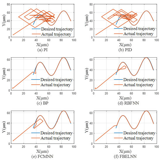
Figure 7.
The comparison of single-cell trajectory using each controller: (a) Use PI as a controller. (b) Use PID as a controller. (c) Use BP as a controller. (d) Use RBFNN as a controller. (e) Use FCMNN as a controller. (f) Use FBELNN as a controller.
Figure 7 shows the effect comparison between the desired trajectory and the expected trajectory of a single cell when PI, PID, BP, RBFNN, FCMNN, and FBELNN are used as controllers, respectively. It can be seen from the figure that when the PI and PID controllers operate a single cell, they cannot control the cell to the desired trajectory in time for a long time, and can move accurately on the desired trajectory after a long time. In contrast, when BP, RBFNN, FCMNN are used as controllers to manipulate single cells, the control effect has been greatly improved, but there is still a problem that the initial manipulation fluctuates greatly and cannot move to the desired trajectory in time. The cell manipulation controller based on FBELNN can move to the desired trajectory in time, and will not produce severe jitter near the trajectory, showing a good control effect.
Figure 8 and Figure 9 show the trajectory errors of X axis and Y axis when using different controllers for single-cell manipulation, so that the control differences of different controllers can be seen more clearly. The trajectory errors of PI and PID controllers in both directions jitter violently before convergence. When BP, RBFNN, and FCMNN are used as controllers, the errors in the X and Y directions can converge to around 0 quickly, but with the change of the trajectory, there will still be slight jitter, which cannot fully fit the desired trajectory. The cell manipulation controller based on FBELNN proposed in this paper can converge the trajectory error to 0 at a faster speed, and still maintain stable control during cell manipulation, with a small trajectory error.
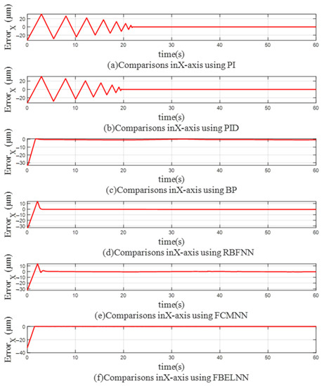
Figure 8.
The trajectory error on the X-axis (single-cell manipulation): (a) Use PI as a controller. (b) Use PID as a controller. (c) Use BP as a controller. (d) Use RBFNN as a controller. (e) Use FCMNN as a controller. (f) Use FBELNN as a controller.
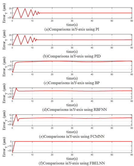
Figure 9.
The trajectory error on the Y-axis (single cell manipulation): (a) Use PI as a controller. (b) Use PID as a controller. (c) Use BP as a controller. (d) Use RBFNN as a controller. (e) Use FCMNN as a controller. (f) Use FBELNN as a controller.
Table 2 shows the root mean square error values (RMSE) of single cell manipulation when using each controller. The error is converted into RMSE and used as the performance evaluation index, which can more clearly and objectively reflect the performance difference of different controllers. It can be seen that under the same experimental parameters, the cell manipulation controller based on FBELNN proposed in this paper has higher control accuracy than other controllers in all controllers, and the RMSE values on X axis and Y axis are 2.8583 × 10⁻⁶ and 2.1381 × 10⁻⁶ respectively. The FCMNN controller has the second smallest RMSE value. Compared with that, the RMSE of the cell manipulation controller proposed in this paper on the X axis and Y axis is reduced by 13% and 19% respectively, which can move the single cell to the desired trajectory in a timely and accurate manner, and better complete the single cell manipulation experiment.
Table 2.
Root mean square error (RMSE) of single-cell manipulation.
5.2. Control Multiple Cells
The holographic optical tweezers system can place and control different optical traps at the same time. According to its advantages, this section will simulate the experiment of using holographic optical tweezers to manipulate multiple cells for cooperative control through MATLAB simulation experiments to verify the cell coordination based on FBELNN. Controller performance and effectiveness for multicellular manipulation control. Configure the same solution environment parameters and controller parameters as in Section 5.1 for simulation experiments. The ideal trajectory for the experiment is designed as:
Set the ideal cell formation to vertical formation. The formation matrix is .
The initial position of captured cells are shown in Table 3.
Table 3.
Initial position of the controlled cells.
The effect of multi-cell cooperative control is shown in Figure 10.
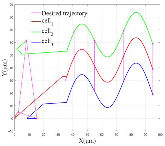
Figure 10.
The effect of multi-cell cooperative control.
Figure 10 demonstrates the effect of multi-cell control using the FBELNN-based cell cooperative controller. It can be seen from the figure that each yeast cell can be manipulated from different initial positions to desired trajectories and form expected desired cell formations. At the same time, the cells can still maintain the preset desired formation during the process of being manipulated to move on the desired trajectory.
Figure 11 shows the relative distances of the three yeast cells in the direction of the X-axis and the direction of the Y-axis during the process of being manipulated. In the direction of the X axis, the initial positions of each cell are similar, and they can move to the expected position at almost the same time. In the direction of the Y axis, since the distance between cell 2 and cell 3 is closer to the expected trajectory, the convergence speed is faster. Cell 1, whose initial position is further away from the desired trajectory, converges slightly slower than the other two cells, but still moves to the desired position in a short time. The effectiveness of the proposed FBELNN-based cell cooperative controller is confirmed.
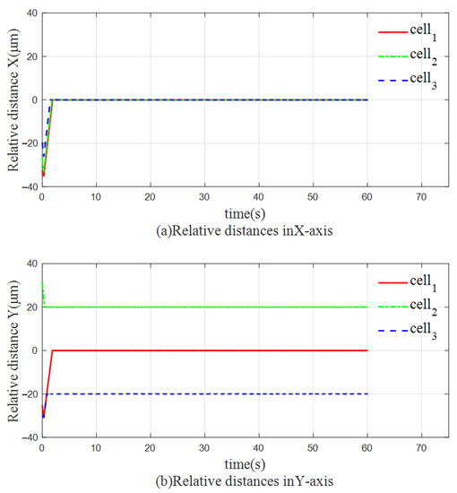
Figure 11.
The relative distance between each yeast: (a) The relative distance of the three cells in the X-axis direction. (b) The relative distance of the three cells in the Y-axis direction.
Figure 12 and Figure 13 show the trajectory errors in the X-axis direction and the Y-axis direction when using different controllers for multi-cell manipulation. It can be clearly seen that the three cells have different trajectory errors during the manipulation control process. When the PI and PID controllers are used, the trajectory errors of the three yeast cells in both directions shake violently before convergence. The farther the initial position of the cells is from the expected trajectory, the slower the trajectory error converges. At the same time, large errors tend to increase the collision risk of multi-cell cooperative control and reduce the control efficiency. When BP, RBFNN, and FCMNN are used as controllers, the errors of the three cells in the X-axis direction and the Y-axis direction can quickly converge to near 0, but as the trajectory changes, the error will still fluctuate near 0. The cell cooperative controller based on the FBELNN proposed in this paper can move multiple cells to the desired trajectory at a faster speed than the above-mentioned controller, and the error convergence speed is extremely fast, which provides the safety of the cell cooperative control. It can complete the cell cooperative control task well and form the expected desired formation.
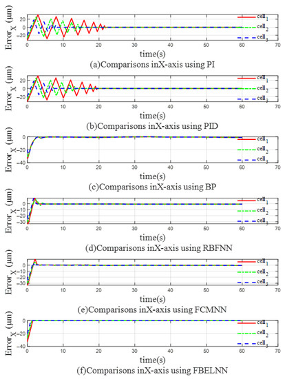
Figure 12.
The trajectory error on the X-axis (multicellular manipulation): (a) Use PI as a controller. (b) Use PID as a controller. (c) Use BP as a controller. (d) Use RBFNN as a controller. (e) Use FCMNN as a controller. (f) Use FBELNN as a controller.
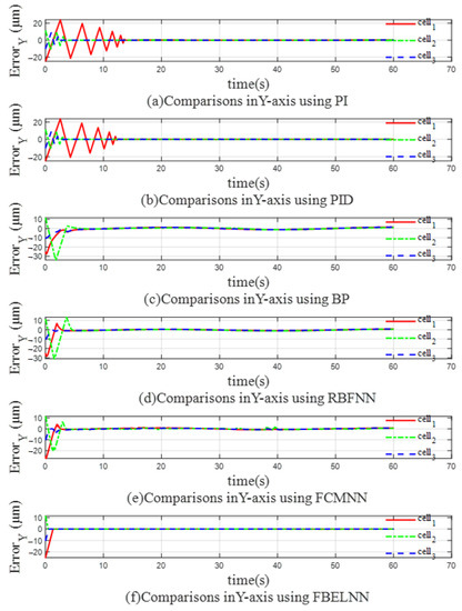
Figure 13.
The trajectory error on the Y-axis (multicellular manipulation): (a) Use PI as a controller. (b) Use PID as a controller. (c) Use BP as a controller. (d) Use RBFNN as a controller. (e) Use FCMNN as a controller. (f) Use FBELNN as a controller.
Table 4 shows the root mean square error values for multi-cell manipulations using each controller. In multi-cell manipulation experiments, RMSE is also used as an evaluation index of control performance. It can be seen that when PI, PID, BP, RBFNN, and FCMNN are used as controllers, their RMSE value ranges are [2.0 × 10⁻⁶, 8.2 × 10⁻⁶], [1.9 × 10⁻⁶, 7.8 × 10⁻⁶], [1.4 × 10⁻⁶, 3.6 × 10⁻⁶], [1.4 × 10⁻⁶, 3.7 × 10⁻⁶], and [1.2 × 10⁻⁶, 3.4 × 10⁻⁶], respectively. Among these controllers, FCMNN has a smaller range of RMSE values and relatively better performance. Then, the FBELNN-based cell cooperative controller proposed in this paper has a large control accuracy advantage compared with the former, and the RMSE value range is between [0.6 × 10⁻⁶, 2.7 × 10⁻⁶]. Compared with the FCMNN controller, the minimum RMSE value and the maximum RMSE value of the cell cooperative controller proposed in this paper are reduced by 51% and 22%, respectively. It greatly improves the control accuracy in multi-cell cooperative control, and is a cell cooperative controller with excellent control performance and stability.
Table 4.
RMSE of multicellular manipulation.
In reality, the cell’s environment might change. For example, changes in the coefficient of viscous resistance will cause changes in the stress of cells. Therefore, according to Table 1, the value of β/k is changed to 0.09 for the experiment. In order to further verify the robustness of the cell cooperative controller based on FBELNN proposed in this paper, the expected trajectory was changed at the same time, and the expected spacing matrix of each yeast cell in the triangle formation was set, . All other experimental parameters remained unchanged.
The new ideal trajectory for the experiment is designed as:
The initial position of the captured cells is shown in Table 5.
Table 5.
Initial position of the captured cells.
The cell trajectories of the vertical formation and the triangular formation are shown in Figure 14 and Figure 15, respectively.
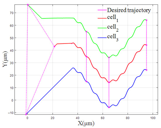
Figure 14.
The cell trajectory of the vertical formation (β/k = 0.09).
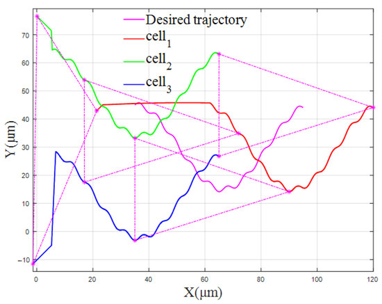
Figure 15.
The cell trajectory of the triangular formation (β/k = 0.09).
Figure 14 and Figure 15 show the trajectories of the FBELNN-based cell cooperative controller manipulating cells and forming vertical or triangular formations under different solution environment coefficients and new ideal desired trajectories. In the new multi-cell experiment, different experimental conditions are set, and the cell cooperative controller can still move the captured cells to the desired formation in time, and can manipulate the three cells to converge from their respective initial positions to the desired spacing position, effectively. The multi-cell cooperative control task in different environments has been completed.
In the experiments in this section, the ideal trajectory defined in this paper can greatly guarantee the safety of the cells during the movement and the effectiveness of the control method. From the simulation results, it can be seen that the multi-cell cooperative controller based on FBELNN has achieved excellent results in controlling cells in different paths. The controller can set different paths and cell formations according to actual needs to realize automatic multi-cell cooperative control tasks. In addition, the adaptability of the FBELNN controller is also very strong, and it can complete the coordinated control of cells in a variety of different environments, which shows that the proposed multi-cell cooperative controller based on FBELNN has good robustness.
6. Conclusions
In this paper, a model of the dynamics of cells trapped by the optical trap generated by holographic optical tweezers is analyzed, and constraints are added to ensure that the cells will not be trapped outside the optical trap. On this basis, a multi-cell cooperative control method is designed, and a multi-cell cooperative controller based on the FBEL neural network is proposed. The controller controls the holographic optical tweezers to generate multiple optical traps to capture the cells, thereby manipulating the cell movement. After a series of cell manipulation simulation experiments, it has been successfully verified. Compared with other previous controllers, the cell cooperative controller proposed in this paper has higher control accuracy, faster convergence speed, and good robustness. There will be no confusion about the trajectory of the captured cells, which greatly improves the safety of multi-cell manipulation experiments. It provides a new idea for efficient and precise cell manipulation automation using holographic optical tweezers.
The obstacle avoidance problem of captured cells in complex environments, however, has not been considered as it pertains to the cell cooperative controller proposed in this paper. At the same time, there are still some unknown disturbances in cell manipulation experiments in reality, and it is necessary to further increase the compensation controller to improve the robustness of the system. These issues will continue to be studied and optimized in future work.
Author Contributions
Methodology, J.Z. and D.-H.W.; Software, J.Z. and P.-S.Z.; Investigation, J.Z. and H.H.; Resources, J.Z.; Writing—original draft, J.Z., H.H. and P.-S.Z.; Writing—review & editing, J.Z. and Y.-K.Y.; Funding acquisition, J.Z. All authors have read and agreed to the published version of the manuscript.
Funding
This research was funded by the Natural Science Foundation of Fujian Province Science and Technology agency under grant number [2020J01285, 2022J05285].
Institutional Review Board Statement
Not applicable.
Informed Consent Statement
Informed consent was obtained from all subjects involved in the study.
Data Availability Statement
Not applicable.
Acknowledgments
This work was supported in part by the Natural Science Foundation (2020J01285, 2022J05285) of the Science and Technology Agency, Fujian, China.
Conflicts of Interest
The authors declare no conflict of interest.
Abbreviations
The following abbreviations are used in this manuscript:
| BP | Back Propagation |
| FBEL | Fuzzy Brain Emotional Learning |
| FBELNN | Fuzzy Brain Emotional Learning Neural Network |
| FCMNN | Fuzzy Cerebellar Model Neural Network |
| PI | Proportional-Integral controller |
| PID | Proportional–Integral–Derivative controller |
| RBF | Radial Basis Function |
| RBFNN | Radial Basis Function Neural Network |
| RMSE | Root Mean Square Error |
| SLM | Space Light Modulator |
References
- Ashkin, A.; Dziedzic, M.; Yamane, T. Optical trapping and manipulation of single cells using infrared laser beams. Nature 1987, 330, 769–771. [Google Scholar] [CrossRef] [PubMed]
- Wang, X.; Chen, S.; Kong, M.; Wang, Z.; Costa, K.D.; Li, R.A.; Sun, D. Enhanced cell sorting and manipulation with combined optical tweezer and microfluidic chip technologies. Lab Chip 2011, 11, 3656–3662. [Google Scholar] [CrossRef] [PubMed]
- Wang, X.; Chen, S.; Chow, Y.T.; Kong, C.W.; Li, R.A.; Sun, D. A microengineered cell fusion approach with combined optical tweezers and microwell array technologies. RSC Adv. 2013, 3, 23589–23595. [Google Scholar] [CrossRef]
- Chowdhury, S.; Švec, P.; Wang, C.; Seale, K.T.; Wikswo, J.P.; Losert, W.; Gupta, S.K. Automated cell transport in optical tweezers-assisted microfluidic chambers. IEEE Trans. Autom. Sci. Eng. 2013, 10, 980–989. [Google Scholar] [CrossRef]
- Fang, T.; Shang, W.; Liu, C.; Xu, J.; Zhao, D.; Liu, Y.; Ye, A. Nondestructive identification and accurate isolation of single cells through a chip with Raman optical tweezers. Anal. Chem. 2019, 91, 9932–9939. [Google Scholar] [CrossRef]
- Keloth, A.; Anderson, O.; Risbridger, D.; Paterson, L. Single cell isolation using optical tweezers. Micromachines 2018, 9, 434. [Google Scholar] [CrossRef]
- Jing, P.; Liu, Y.; Keeler, E.G.; Cruz, N.M.; Freedman, B.S.; Lin, L.Y. Optical tweezers system for live stem cell organization at the single-cell level. Biomed. Opt. Express 2018, 9, 771–779. [Google Scholar] [CrossRef]
- Rodrigues, M.; Kosaric, N.; Bonham, C.A.; Gurtner, G.C. Wound healing: A cellular perspective. Physiol. Rev. 2019, 99, 665–706. [Google Scholar] [CrossRef]
- Zhong, M.C.; Wei, X.B.; Zhou, J.H.; Wang, Z.Q.; Li, Y.M. Trapping red blood cells in living animals using optical tweezers. Nat. Commun. 2013, 4, 1–7. [Google Scholar] [CrossRef]
- Chung, Y.C.; Chen, P.W.; Fu, C.M.; Wu, J.M. Particles sorting in micro-channel system utilizing magnetic tweezers and optical tweezers. J. Magn. Magn. Mater. 2013, 333, 87–92. [Google Scholar] [CrossRef]
- Wu, J. Acoustical tweezers. J. Acoust. Soc. Am. 1991, 89, 2140–2143. [Google Scholar] [CrossRef] [PubMed]
- Samadi, M.; Alibeigloo, P.; Aqhili, A.; Khosravi, M.A.; Saeidi, F.; Vasini, S.; Ghorbanzadeh, M.; Darbari, S.; Moravvej-Farshi, M.K. Plasmonic tweezers: Towards nanoscale manipulation. Opt. Lasers Eng. 2022, 154, 107001. [Google Scholar] [CrossRef]
- Kotnala, A.; Kollipara, P.S.; Zheng, Y. Opto-thermoelectric speckle tweezers. Nanophotonics 2020, 9, 927–933. [Google Scholar] [CrossRef] [PubMed]
- Marzo, A.; Drinkwater, B.W. Holographic acoustic tweezers. Proc. Natl. Acad. Sci. USA 2019, 116, 84–89. [Google Scholar] [CrossRef] [PubMed]
- Xie, M.; Shakoor, A.; Wu, C. Manipulation of biological cells using a robot-aided optical tweezers system. Micromachines 2018, 9, 245. [Google Scholar] [CrossRef]
- Xiong, T.; Wang, Z.; Liu, Y.; Zhou, Z. Research progress of optical tweezers in the detection of single cell and single-molecule properties. Laser J. 2021, 42, 7–17. [Google Scholar]
- Cheah, C.; Li, X.; Yan, X.; Sun, D. Simple PD Control Scheme for Robotic Manipulation of Biological Cell. IEEE Trans. Autom. Control 2015, 60, 1427–1432. [Google Scholar] [CrossRef]
- Xie, M.; Li, X.; Wang, Y.; Liu, Y.; Sun, D. Saturated PID Control for the Optical Manipulation of Biological Cells. IEEE Trans. Control Syst. Technol. 2018, 26, 1909–1916. [Google Scholar] [CrossRef]
- Aguilar-Ibañez, C.; Suarez-Castanon, M.S.; Rosas-Soriano, L.I. A simple control scheme for the manipulation of a particle by means of optical tweezers. Int. J. Robust Nonlinear Control 2011, 21, 328–337. [Google Scholar] [CrossRef]
- Zeng, G.Q.; Xie, X.Q.; Chen, M.R.; Weng, J. Adaptive population extremal optimization-based PID neural network for multivariable nonlinear control systems. Swarm Evol. Comput. 2019, 44, 320–334. [Google Scholar] [CrossRef]
- Yang, H.; Liu, J. An adaptive RBF neural network control method for a class of nonlinear systems. IEEE/CAA J. Autom. Sin. 2018, 5, 457–462. [Google Scholar] [CrossRef]
- Dong, Z.; Bao, T.; Zheng, M.; Yang, X.; Song, L.; Mao, Y. Heading control of unmanned marine vehicles based on an improved robust adaptive fuzzy neural network control algorithm. IEEE Access 2019, 7, 9704–9713. [Google Scholar] [CrossRef]
- Liu, Y.J.; Zeng, Q.; Tong, S.; Chen, C.P.; Liu, L. Adaptive neural network control for active suspension systems with time-varying vertical displacement and speed constraints. IEEE Trans. Ind. Electron. 2019, 66, 9458–9466. [Google Scholar] [CrossRef]
- Bai, W.; Zhou, Q.; Li, T.; Li, H. Adaptive reinforcement learning neural network control for uncertain nonlinear system with input saturation. IEEE Trans. Cybern. 2019, 50, 3433–3443. [Google Scholar] [CrossRef] [PubMed]
- Liu, Y.J.; Zhao, W.; Liu, L.; Li, D.; Tong, S.; Chen, C.P. Adaptive neural network control for a class of nonlinear systems with function constraints on states. IEEE Trans. Neural Netw. Learn. Syst. 2021, 1–10. [Google Scholar] [CrossRef]
- Khorashadizadeh, S.; Zadeh, S.M.H.; Koohestani, M.R.; Shekofteh, S.; Erkaya, S. Robust model-free control of a class of uncertain nonlinear systems using BELBIC: Stability analysis and experimental validation. J. Braz. Soc. Mech. Sci. Eng. 2019, 41, 1–12. [Google Scholar] [CrossRef]
- Ebrahimnejad, A. An effective computational attempt for solving fully fuzzy linear programming using MOLP problem. J. Ind. Prod. Eng. 2019, 36, 59–69. [Google Scholar] [CrossRef]
- Sori, A.A.; Ebrahimnejad, A.; Motameni, H. The fuzzy inference approach to solve multi-objective constrained shortest path problem. J. Intell. Fuzzy Syst. 2020, 38, 4711–4720. [Google Scholar] [CrossRef]
- Ebrahimnejad, A.; Nasseri, S. Linear programmes with trapezoidal fuzzy numbers: A duality approach. Int. J. Oper. Res. 2012, 13, 67–89. [Google Scholar] [CrossRef]
- Lin, C.; Chung, C. Fuzzy brain emotional learning control system design for nonlinear systems. Int. J. Fuzzy Syst. 2015, 17, 117–128. [Google Scholar] [CrossRef]
- Muthusamy, P.K.; Garratt, M.; Pota, H.; Muthusamy, R. Realtime Adaptive Intelligent Control System for Quadcopter UAV with Payload Uncertainties. IEEE Trans. Ind. Electron. 2021, 69, 1641–1653. [Google Scholar] [CrossRef]
- Lin, Q.; Xu, Z.; Lin, C. Battery-Supercapacitor State-of-Health Estimation for Hybrid Energy Storage System Using a Fuzzy Brain Emotional Learning Neural Network. Int. J. Fuzzy Syst. 2022, 24, 12–26. [Google Scholar] [CrossRef]
- Pang, H.; Li, W.; Wang, X.; Zhao, S.; Zhou, Z. The latest research and applications of holographic optical tweezers. Laser J. 2019, 40, 1–6. [Google Scholar]
- Huang, Y.; Zhang, Z.; Menq, C. Minimum-variance Brownian motion control of an optically trapped probe. Appl. Opt. 2009, 48, 5871–5880. [Google Scholar] [CrossRef]
- Arai, F.; Yoshikawa, K.; Sakami, T.; Fukuda, T. Synchronized laser micromanipulation of multiple targets along each trajectory by single laser. Appl. Phys. Lett. 2004, 85, 4301–4303. [Google Scholar] [CrossRef]
- Gittes, F.; Schmidt, C. Signals and noise in micromechanical measurements. Methods Cell Biol. 1997, 55, 129–156. [Google Scholar]
- Wu, Y.; Sun, D.; Huang, W. Mechanical force characterization in manipulating live cells with optical tweezers. J. Biomech. 2011, 44, 741–746. [Google Scholar] [CrossRef]
- Dong, X. Robotic Manipulation of Biological Cells Based on Optical Tweezers; Shenzhen University: Shenzhen, China, 2018. [Google Scholar]
- Zhou, W. The influence of viscous resistance of fluid on body motion. Tech. Phys. Teach. 2009, 17, 27–28. [Google Scholar]
- Zhang, Z.; Cui, G. Hydrodynamics; Tsinghua University Press: Beijing, China, 1998. (In Chinese) [Google Scholar]
- Wu, Y.; Chen, H.; Sun, D.; Huang, W. Force characterization of live cells in automated transportation with robot-tweezers manipulation system. 2010 IEEE International Conference on Mechatronics and Automation. 2010, 1913–1918. [Google Scholar]
- Oertel, H. Prandtl’s Essentials of Fluid Mechanics.; Springer: New York, NY, USA, 2004. [Google Scholar]
- Hu, S.; Chen, S.; Chen, S.; Xu, G.; Sun, D. Automated transportation of multiple cell types using a robot-aided cell manipu-lation system with holographic optical tweezers. IEEE/ASME Trans. Mechatron. 2017, 22, 804–814. [Google Scholar] [CrossRef]
- Dai, C.; Zhang, Z.; Lu, Y.; Zhao, Q.; Ru, C.; Sun, Y. Robotic manipulation of deformable cells for orientation control. IEEE Trans. Robot. 2020, 36, 271–283. [Google Scholar] [CrossRef]
- Hu, S.; Sun, D. Automatic transportation of biological cells with a robot-tweezer manipulation system. Int. J. Robot. Res. 2022, 30, 1681–1694. [Google Scholar] [CrossRef]
- Su, H.; Qi, W.; Chen, J.; Zhang, D. Fuzzy Approximation-based Task-Space Control of Robot Manipulators with Remote Center of Motion Constraint. IEEE Trans. Fuzzy Syst. 2022, 30, 1564–1573. [Google Scholar] [CrossRef]
- Xu, Z.; Lin, Q.; Lin, C.M. Online health estimate of hybrid energy storage system based on fuzzy brain emotional learning neural networks. In Proceedings of the 2020 International Conference on System Science and Engineering, Kagawa, Japan, 31 August–3 September 2020; pp. 511–516. [Google Scholar]
- Shang, M. Research on Cooperative Formation Control Technology for Multi-Mobile Robots; Beijing University of Posts and Telecommunications: Beijing, China, 2021. [Google Scholar]
- Hsu, C.F. Intelligent total sliding-mode control with dead-zone parameter modification for a DC motor driver. IET Control Theory Appl. 2014, 8, 916–926. [Google Scholar] [CrossRef]
Disclaimer/Publisher’s Note: The statements, opinions and data contained in all publications are solely those of the individual author(s) and contributor(s) and not of MDPI and/or the editor(s). MDPI and/or the editor(s) disclaim responsibility for any injury to people or property resulting from any ideas, methods, instructions or products referred to in the content. |
© 2022 by the authors. Licensee MDPI, Basel, Switzerland. This article is an open access article distributed under the terms and conditions of the Creative Commons Attribution (CC BY) license (https://creativecommons.org/licenses/by/4.0/).