Article

Robust Facial Expression Recognition Using an Evolutionary Algorithm with a Deep Learning Model

by
Mayuri Arul Vinayakam Rajasimman
1,
Ranjith Kumar Manoharan
2,
Neelakandan Subramani
3,*,
Manimaran Aridoss
4 and
Mohammad Gouse Galety
5
1
School of Computing Science and Engineering, VIT Bhopal University, Bhopal 466114, India
2
Department of Mathematics, Amrita School of Engineering, Amrita Vishwa Vidyapeetham, Chennai 601103, India
3
Department of Computer Science and Engineering, R.M.K Engineering College, Kavaraipettai 601206, India
4
School of Advanced Sciences, VIT-AP University, Amaravati 522237, India
5
Department of Information Technology and Computer Science, Catholic University in Erbil, Erbil 44001, Kurdistan Region, Iraq
*
Author to whom correspondence should be addressed.
Appl. Sci. 2023, 13(1), 468; https://doi.org/10.3390/app13010468
Submission received: 14 November 2022 / Revised: 10 December 2022 / Accepted: 24 December 2022 / Published: 29 December 2022

Abstract

:
The most important component that can express a person’s mental condition is facial expressions. A human can communicate around 55% of information non-verbally and the remaining 45% audibly. Automatic facial expression recognition (FER) has now become a challenging task in the surveying of computers. Applications of FER include understanding the behavior of humans and monitoring moods and psychological states. It even penetrates other domains—namely, robotics, criminology, smart healthcare systems, entertainment, security systems, holographic images, stress detection, and education. This study introduces a novel Robust Facial Expression Recognition using an Evolutionary Algorithm with Deep Learning (RFER-EADL) model. RFER-EADL aims to determine various kinds of emotions using computer vision and DL models. Primarily, RFER-EADL performs histogram equalization to normalize the intensity and contrast levels of the images of identical persons and expressions. Next, the deep convolutional neural network-based densely connected network (DenseNet-169) model is exploited with the chimp optimization algorithm (COA) as a hyperparameter-tuning approach. Finally, teaching and learning-based optimization (TLBO) with a long short-term memory (LSTM) model is employed for expression recognition and classification. The designs of COA and TLBO algorithms aided in the optimal parameter selection of the DenseNet and LSTM models, respectively. A brief simulation analysis of the benchmark dataset portrays the greater performance of the RFER-EADL model compared to other approaches.

1. Introduction

Facial expressions have a significant role in presenting the emotions of humans, which might affect day-to-day life by changing our memory, attention, and perceptions. Facial expressions might precisely express the true emotions of others. Humans can learn the inner thoughts of others via facial expressions [1]. Psychologists reported that facial expression is prominent in the day-to-day interactions of humans, making up 55%, of communication, far greater than the written language (7%), speech (38%), etc. [2]. On the other hand, facial expressions are unaffected by age, race, gender, or cultural background and follow from facial muscle movements [3]. Consequently, facial expressions are an effective means of identifying emotions. The study of facial expression detection is vital for progressing artificial intelligence and other fields, and it is based on computer technology that could allow intelligent devices such as robots to identify and better understand our emotions, accomplish barrier-free communication between machines and humans, actively judge human emotion, and better serve humans [4].
Currently, automated FER is the most important task in the field of computer science [5]. An expression could be transported via communication and gestures. It does not depend on the facial expressions of humans. The authors emphasize that a person could orally transmit around 7% of data context, whereas 38% are transported via rhythm, voice tone, and how slowly or speedily a person talks [6]. The applications of facial expressions cover a wide swatch of functions in our society and are not constrained to this field. In medical science, FER is useful for bipolar patients. Physicians try to monitor and detect the behaviors of a patient, like how they behave during their disease and how a bipolar patient feels [7]. An intelligent FER technique such that face images are provided as input and could identify the expression of humans. There exist, overall, eight expressions, including happy, fearful, sad, surprised, angry, neutral, disgusted, and contempt-filled [8]. FER uses a deep learning (DL)-based techniques to help it extract facial expressions and features, which greatly improves its performance. However, FER is prone to complex problems, such as slow recognition speed, trouble extracting facial features, and low recognition accuracy. The key concept of the DL technique is to construct an artificial neural network (ANN) by continuous training of enormous quantities of information to satisfy certain requirements [9]. The goal of a DL algorithm is to retrieve the information confined in the input hierarchically through the construction of multi-layer neural networks (MNNs); this relates to the outlining of hidden layers among the input and output layers of a single computing layer perceptron as an internal description of “input mode”, such that it becomes a multilayer perceptron (MLP), and the neurons between neighboring layers are interconnected with one another. [10]. Applied science in digital image processing and visualization is now one of the fastest-growing areas of information technology. It has various applications in medical imaging, remote sensing, industrial inspection, computer vision and robotics, image editing, and information visualization. With the rapid growth of multimedia content in social media and smartphone applications, innovative image processing tools and programs for creating featured photographs to improve the aesthetics, entertainment, publicity, and security of these applications are gaining popularity.
We developed the Robust Facial Expression Recognition using an Evolutionary Algorithm with Deep Learning (RFER-EADL) model. As a preprocessing step, the RFER-EADL approach employs histogram equalization (HE). In addition, for feature extraction, the chimp optimization algorithm (COA) with a densely linked network (DenseNet-169) model is applied. Finally, for expression identification and classification, a teaching and learning-based optimization (TLBO) model with long short-term memory (LSTM) is used. A complete experimental assessment of the benchmark dataset portrays the greater performance of the RFER-EADL model compared to other approaches.

2. Literature Review

Rajan et al. [11] examined a new DL infrastructure that integrates CNN with LSTM cells for real-time FER. The novel infrastructure comprises three essential features: (1) Two distinct pre-processed approaches are utilized for handling illumination differences and for preserving subtle edge data of all the images. (2) The pre-processing images are inputted into two individual CNN infrastructures that remove the spatial features very efficiently. (3) The spatial feature maps in two separate CNN layers are fused and combined with an LSTM layer which that removes temporal connections betwixt the succeeding frames. In [12], a novel technique for human FER that executes an improved type of cat swarm optimization (CSO) technique, named improved CSO (ICSO), was presented. An input image provided to the projected method retrieved the same images in the dataset and recognizes the person’s emotional state with facial expressions. The deep features that occurred in the face images were extracted utilizing the DCNN system. An ICSO was presented for selecting an optimum feature in the face image which individually separated the facial expression of persons.
Wang et al. [13] examined suppressing the uncertainty by an easy yet effective self-cure network (SCN). The SCN suppresses the uncertainty in two distinct features, (i) a self-attention process on the FER dataset for weighting all the instances from training with ranking regularization, and (ii) a careful relabeling process for labelling the instances with the lowest rankings. Li et al. [14] are investigating an end-to-end network with automatic FER. A novel network infrastructure is made up of reconstruction, attention, feature extraction, and classifier modules. Using image texture, LBP recognizes facial movements and improves network performance.
Cheng and Zhou [15] introduced an expression detection method of enhanced VGG-DCNN. According to the VGG-19; this method improves network infrastructure and network constraints. Most expression datasets were ineffectual for training the total networks in the beginning because of the lack of appropriate data. This work utilizes migration-learning approaches for overcoming the lack of image trained instances. In [16], We introduce E2-Capsnet, a double-enhanced capsule neural network that takes FER into account while also being U-aware, in this article. E2-Capsnet advances two enhancement components that benefit FER through dynamic routing between capsules. In this context, the CNN is a vital part of the development process because it pays special attention to the areas of expressions that are actually doing work. The secondary development component is the Capsnet with several convolutional layers that improve the feature representations.
Kim et al. [17] examined a novel approach for the FER technique that is dependent upon hierarchical DL. The extracted features are combined with geometric features from a hierarchical infrastructure in a network based on presence features. The presence-feature-based 124-node network extracts global facial features from preprocessed LBP images. The geometric feature-constructed network taught the action units (AUs), the muscles most actively involved in the creation of facial expressions, to recognize the coordinate transformation. Zhu et al. [18] presented few-shot learning for developing a DL method known as the convolutional relation network (CRN) for FER in the field. By comparing the feature similarity between those instances, this technique allows for the discovery of novel classes that share some traits with instances of the correct emotion class. The classifier learns a metric space via distance computation, and the deep expression features’ ability to discriminate is then used to improve the network’s predictive capabilities.
According to Shuai Liu [19], multimodal research is currently being used in a variety of fields. Existing emotion identification algorithms are incapable of resolving modal conflict and fail to take into account the internal interactions of several modalities. As a result, resolving modal conflict through the fusion of different modalities is critical to the development of multimodality. In this study, we introduce an attention mechanism to fuse many modalities, since attention mechanisms are key in deep learning. A GNN for FER was proposed by Liu S et al. [20]. The approach divides the human face into six separate sections, extracts feature key points from each segment evenly using “local visual cognition”, shows the internal relationships between feature key points using “regional cooperative recognition”, and lastly constructs a GNN model to realize FER. By comparing it to similar algorithms, this method proved FER’s effect and increased the possible uses of neural network models. It also improved the interpretability of GNN’s cognitive science data. Table 1 shows the objectives and significant results of existing works.
A lot of research has gone into making FER systems reliable because they can be used in a wide range of fields, such as computer vision, image processing, and pattern classification. A very hard problem to solve in these is getting the computers to be able to see human faces and figure out what emotions they are showing, such as anger, happiness, neutrality, sadness, and disgust.

3. The Proposed Model

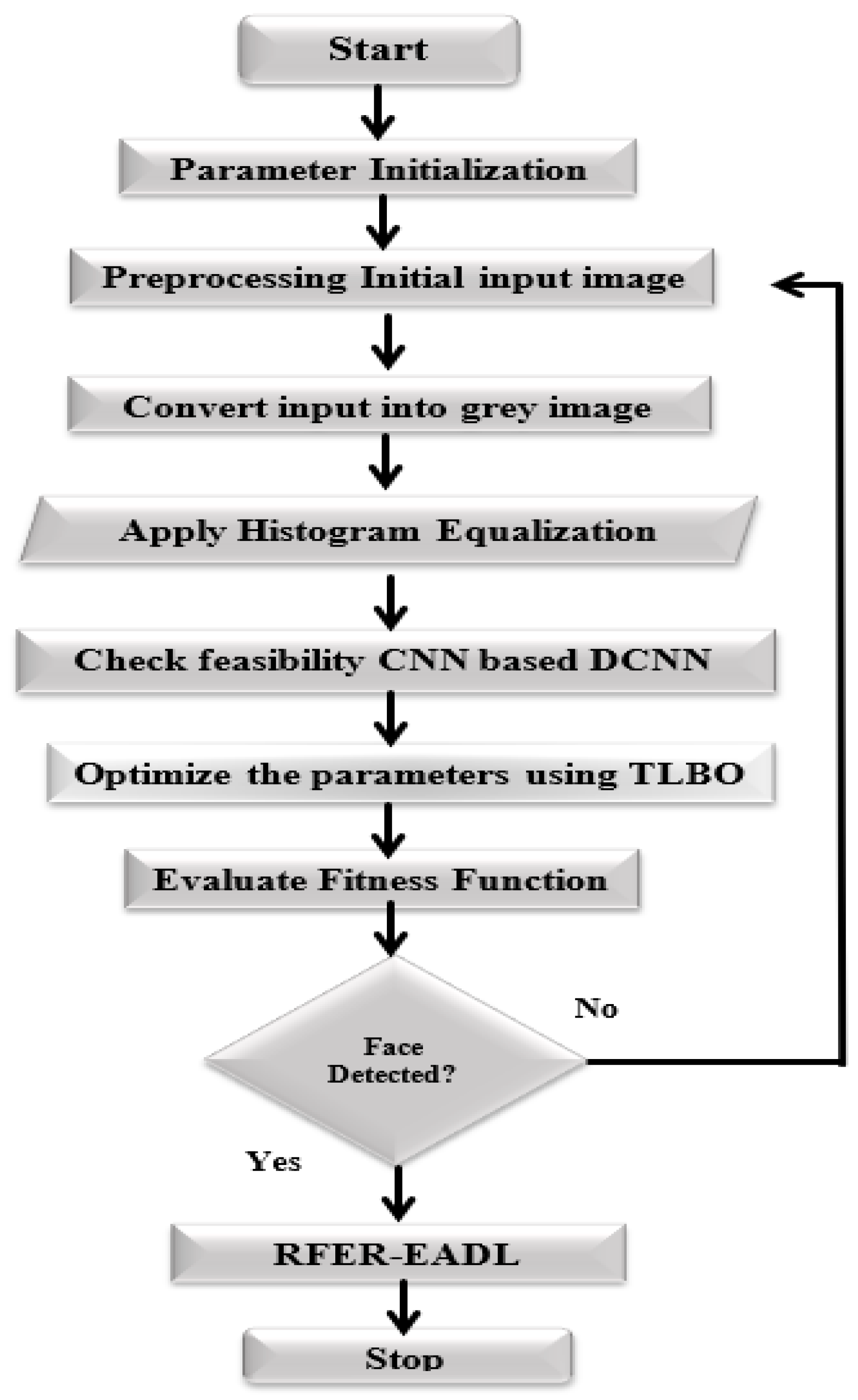
During this investigation, a novel RFER-EADL technique was established for emotion recognition in facial images. First, the presented RFER-EADL technique uses an HE process. The COA model, along with the DenseNet-169 model, is then used to extract features. Finally, the TLBO with an LSTM model is used to recognize and categorize emotional facial expressions. Figure 1 depicts RFER-EADL’s block diagram.

3.1. Histogram Equalization

Histogram equalization can be used to change the contrast of a digital image. Each pixel’s individual processing results in the creation of a new image. The image’s cumulative histogram is used in this modification. Histogram equalization attempts to “spread out” the histogram in order to achieve a more uniform distribution of intensities across all potential value ranges. Equalization is useful for photos with little to no contrast. The procedure is straightforward, and it is carried out by a computer.
X(i,j) is a representation of the intensity at the coordinates (I,j) that satisfy the condition. The intensity values of an image are random variables with values ranging from 0 to L1. Let X signify the input image and L signify the total number of distinct grey levels in the dynamic range. (I, j) ϵ{X0, X1,…, XL1}. The discrete function that defines the histogram h for a digital image is given in the equation below h(Xk) = nk, where
  • The kth intensity level in the [0, L1] range is represented by the value Xk.
  • If nk is large, the input image has a large number of pixels.
The brightness and contrast are distinct even amongst images of similar people with similar expressions. The HE processes has been executed for all the images for reducing this difference [24]. The mean value of normalization images was closer. Normalized Z-score was also used for these images via Equation (1), for enhancing the contrast.
x = x μ σ
in which x stands for the value of a novel pixel, x refers the value of the original, μ stands for the average pixel value in all instances of an image, and is the standard deviation of those pixel values. Pixels are the image’s constituents.

3.2. Feature Extraction

For the optimal derivation of the features related to the facial images, the DenseNet-169 model is utilized. The CNN is applied to extract useful features from the raw information [25,26,27,28,29]. The primary layers utilized in the deep convolutional network are the max-pooling, convolutional, and FC layers. In a single-layer CNN network, feature extraction can be attained through a convolutional operator using the filter on the input signal. In CNN, the activation of every unit characterizes the convolved kernel or filter via an input signal. It is assumed that the filter in the convolutional layer in this network acts as a feature extractor and progressively highlights certain features in the topmost layer of the network. While employing a temporal sequence (sensor signal), a 1D kernel is utilized in temporal convolution [30,31]. Generally, feature extraction can be determined as a 2D displacement operation in the convolutional layer:
a i l + 1 = σ ( j = 1 J l w j l .   a i + j l + b i l )
Now, the variable a i l + 1 indicates the feature map i to convolution layer l + 1 , and w l represents the weighted matrices of kernel function in the convolution layer l that generates the next input layer via convoluting with the output of the preceding layer, a i + i l . The variable b i l refers to the bias vector. Another significant layer in the convolutional network is the pooling layer. These layers perform a kind of nonlinear down-sampling; hence, they decrease the size of the dataset by integrating the output related to the adjusted neuron in the convolutional layer. After every convolution layer, a pooling layer is positioned in a period to summarize the output of the convolutional layer on the network [32].
This study presented the effect of having any connections between CNN layers. Next, researchers tried to construct a deep CNN that has the shortest connections between layers nearer the input and output. The outcome showed that the deep CNN model has the shortest connections between layers, and is more precise and effective to train (ResNet). ResNet has skip-connections amongst deep layers that bypass the non-linear transformation layer. As an alternative to ResNets, researchers introduced DenseNet, which has a fully connected layer [33].
In DenseNet, layers have direct connections to other succeeding layers. Consequently the l t h layer attains the function chart of each preceding layer X 0 to X l 1 , as in Equation (3).
X l = H l ( [ X 0 , X 1 ,   X l 1 ] )
[ X 0 , X 1 ,   X l 1 ] represents the feature-map spectrum generated in the layers 0,1. l 1 . Researchers trained the DenseNet model using ImageNet datasets; the test outcome was from 5.29% to 7.71% errors in prediction [34]. The DenseNet model with ImageNet pre-trained weights caused the growth rate for each network to be k = 32 . The DenseNet model was used in the study where the global average pooling had shape ( 1 , 1664 ) .

3.3. Hyperparameter Tuning

To optimally modify DenseNet’s hyperparameters, the COA was used. COA is simulated by the hunting nature of chimps [35,36,37,38]. The primary two roles in team hunting, such as chase and driver scenarios, are statistically defined as:
d = | c . x p r e y ( t ) m . x c h i m p ( t ) |
x c h i m p ( t + 1 ) = x p r e y ( t ) a d
t implies the count of present iterations; a ,   m , and c are co-efficient vectors; x p r e y defines the prey point vector; and x c h i m p stands for the chimp point vector. The vectors m , and c are computed by Equations (6)–(8), correspondingly.
a = 2 f r 1 f
c = 2 r 2
m = C h a o t i c v a l u e
f reduces the non-linearly by an iterative procedure in 2.5 to 0 (either exploration or extraction stages), but r 1 and r 2 are arbitrary vectors from the interval of one and zero. Likewise, m defines the vector which is computed dependent upon a turbulent map [30,31]. This vector represents the outcome of the chimp’s sexual stimulus on the hunting procedure.
The stochastic populace generation is a primary stage of the ChOA technique. Afterward, the chimps are arbitrarily decided into four independent groups—namely attacker, barrier, driver, and chaser. All the group approaches define the place-upgrading process of individual chimps by defining the f vector, but every group’s purpose is estimating the potential prey’s place [39,40,41,42]. The c and m vectors were tuned adaptably and improve the local minimum avoidance and rate of convergence.
Chimps (chaser, driver, and barrier) search for prey and then surround it. The hunting procedure is commonly implemented by attacking chimps [40]. The chasing stimuli, obstacles, and chimps at times contribute to the hunting procedure. To mathematically act out chimps’ performance, it can be considered that the primary attackers (an optimum solution accessible), the pursuer, the stimulus, and the obstacle are more aware of the prey’s place [43,44,45]. Therefore, the four optimum solutions were achieved, and storage and another chimp were forced to update their places based on optimum chimp places. This connection is written by Equations (9)–(11).
d A t t a c k e r = | c 1 x A t t a c m 1 x | , d B a r r i e r = | c 2 x B a r r i e r m 2 x | d C h a s e r = | c 3 x C h a s e r m 3 x | , d D r i v e r = | c 4 x D r i v e r m 4 x |
x 1 = x A t t a c k e r a 1 ( d A t t a c k e r ) , x 2 = x B a r r i e r a 2 ( d B a r r i e r ) x 3 = x C h a s e r a 3 ( d C h a s e r ) , x 4 = x D r i v e r a 4 ( d D r i v e r )
x ( t + 1 ) = x 1 + x 2 + x 3 + x 4 4
x1 is the best solution; x2 is the second-best solution; x3 is the third-best solution; x4 is the fourth-best solution. m mathematically processes chimps’ chaotic performance in the hunting last step for obtaining further meat, and afterward, further social favors, such as grooming.

3.4. Facial Expression Classification

To carry out the FER method, the LSTM model was utilized in this study. LSTM is a kind of network structure that is intended to resolve the RNN problem of an unstable gradient that limits its use for modeling temporal dependency and long-term activity sequences with those data gained from a sensor [46,47,48]. Thereby, the LSTM architecture could learn long-term dependency that is impossible via RNN. The building block of LSTM is the cell state. With the grouping of memory cells, the LSTM controls the input data flow. It can be obtained by the gate structure that could optionally permit data to be entered. The LSTM comprises three gates for controlling the values of the cell state. Figure 2 depicts the infrastructure of LSTM.
The initial gate of LSTM determines which data should be clear from the cell position. The outcome can be performed using a sigmoid layer named the “forget gate”. The output of these gates is demonstrated in Equation (12), where u t indicates the input vector at time t (existing input); h t 1 represents the history or memory value from the preceding time step; w ( u . )   and   w ( h . ) indicates the weight matrices, correspondingly, associated with the u   and   h values; and b denotes the bias vector that determines the transformation of the specific gate [49]. This gate output 0 or 1 value for all the numbers in the cell state c t 1 concerning h t 1 and u t . The value of 0 signifies “completely forgetting these states”, whereas the value of 1 signifies completely keeping these states.
f t = σ f ( w u f u t + w h f b t 1 + b f )
The next gate is intended to decide which novel information needs to be stored in all the cell states. The procedure has two phases. Initially, there exists a sigmoid layer named the input gate to determine what value needs to be upgraded. Next, it generates a vector named g t that is added to the cell state with the help of a hyperbolic tangent layer as follows:
i t = σ i ( w u i u t + w h i b t 1 + b i )
g t =   tan h   ( w u g u t + w h g b t 1 + b c )
Then, the oldest cell state C t 1 is enhanced by the new cell state, g t .
c t = f t c t 1 + i t g t
o t = σ ( w u o u t + w h o b t 1 + b o )
Consequently, the value of output variable b t (novel history) is upgraded in all the steps based on the value of cell state 0 t and the output value 0 t :
b t = 0 t   tan h   ( c t )
To enhance the efficacy of the LSTM model, the TLBO algorithm is exploited for the hyperparameter tuning process. TLBO technique is a novel metaheuristic algorithm that enhances the knowledge level by simulating “teaching” and “learning” from people’s learning procedures [50,51,52]. TLBO is the feature of some parameters and performs well. TLBO is well implemented in mechanical-design-optimized, heat-exchanger-optimized, thermoelectric-cooler-optimized applications.
For facilitating understanding, the subsequent are any basic explanations of the TLBO technique:
Definition 1: 
Search space for individual (solution vector)  X = ( x 1 ,   x 2   , ,   x D ) named learners; x i   ( i = l , 2   ,   D ) is the i course for students.
Definition 2: 
The group of students is termed a class.
Definition 3: 
Students with the maximum level (fitness) X b e s t = ( x 1 b e s t ,   x 2 b e s t , ,   x D b e s t ) are termed X t e a c h e r . In the TLBO technique, the class is equivalent to the population from GA, a student is equivalent to an individual, and the teacher is an individual with the maximum adaptive value. The task of teachers is to teach hard and promote the average level of students in the class. The students enhance their skills by learning from teachers and interconnecting with classmates. The TLBO technique was separated into two stages: the teaching stage and the learning stage as shown in below Algorithm 1.
Algorithm 1: Teaching stage
For   each   learner   X J   = ( x 1 j , x 2   j ,   , x D j ) ( j = 1 , 2 ,   ,   N P ) Do
x i J , n e w   = x j , o l d + rand ( ) x ( x i b e s t T F × M e a n 1 ) , j = 1 , 2 , , N P , i = 1 , 2 , , D
If   X j , new X j . o l d then
X j = X j , n e w
End if
End for
Here, x l j , old and x l j new i imply the knowledge level of X j , S   i before and after teaching, correspondingly. Rand ( ) defines the arbitrary sum between zero and one.
The learning technique is as follows:
T F = r o u n d [ 1 + r a n d (   ) ] ,   M e a n i = 1 N P j = 1 N P x i j ,
NP refers the entire count of students, and D defines the count of courses (dimensional) as shown in below Algorithm 2.
Algorithm 2: Learning stage
For   each   learner   X j j = 1 , 2 N P ,
Choose   a   student   X *   at   arbitrary   from   the   class   ( j k )
If   X j   is   higher   to   X * then
X j , n e w = X j , o l d + r a n d 1 ( 1 ,   D ) x ( X j X k )
Else
X j , n ε w = X j , o I d r a n d ( 1 ,   D ) x ( X   k X j )
E n d
if   X j , n e w   i s   s u p e r i o r   t o   X j , o l d then
X   j = X j , n e w |
End if
End for
To improve classification results, a fitness function (FF) will be developed using the TLBO strategy. A positive integer is chosen to denote that the candidate solutions are superior. For the purposes of this article, the FF will be defined as the reduction in the classifier’s overall error rate, as demonstrated by Equation (19).
f i t n e s s ( x i ) = C l a s s i f i e r E r r o r R a t e ( x i ) = n u m b e r   o f   m i s c l a s s i f i e d   s a m p l e s T o t a l   n u m b e r   o f   s a m p l e s 100
TLBO is an algorithm that does not require input parameters. TLBO only requires the parameters of population and generation size. In a reasonable amount of time, the TLBO algorithm achieves optimal results when solving numerous discrete and continuous optimization problems [53,54,55]. We propose the ChOA Algorithm, which was inspired by TLBO. In TLBO, there are two distinct phases: teaching and learning. The ChOA algorithm consists of just one step. It is simpler to implement than TLBO. In the first step, candidates with random values are added to the population, as show in Figure 3. Candidates’ fitness levels are determined by a fitness function [56]. The optimal candidate among the candidates is identified (Xbest). Furthermore, the candidate with the poorest fitness is identified (Xworst) [57]. The candidate solutions in the population are modified based on the preceding equation.

4. Results and Discussion

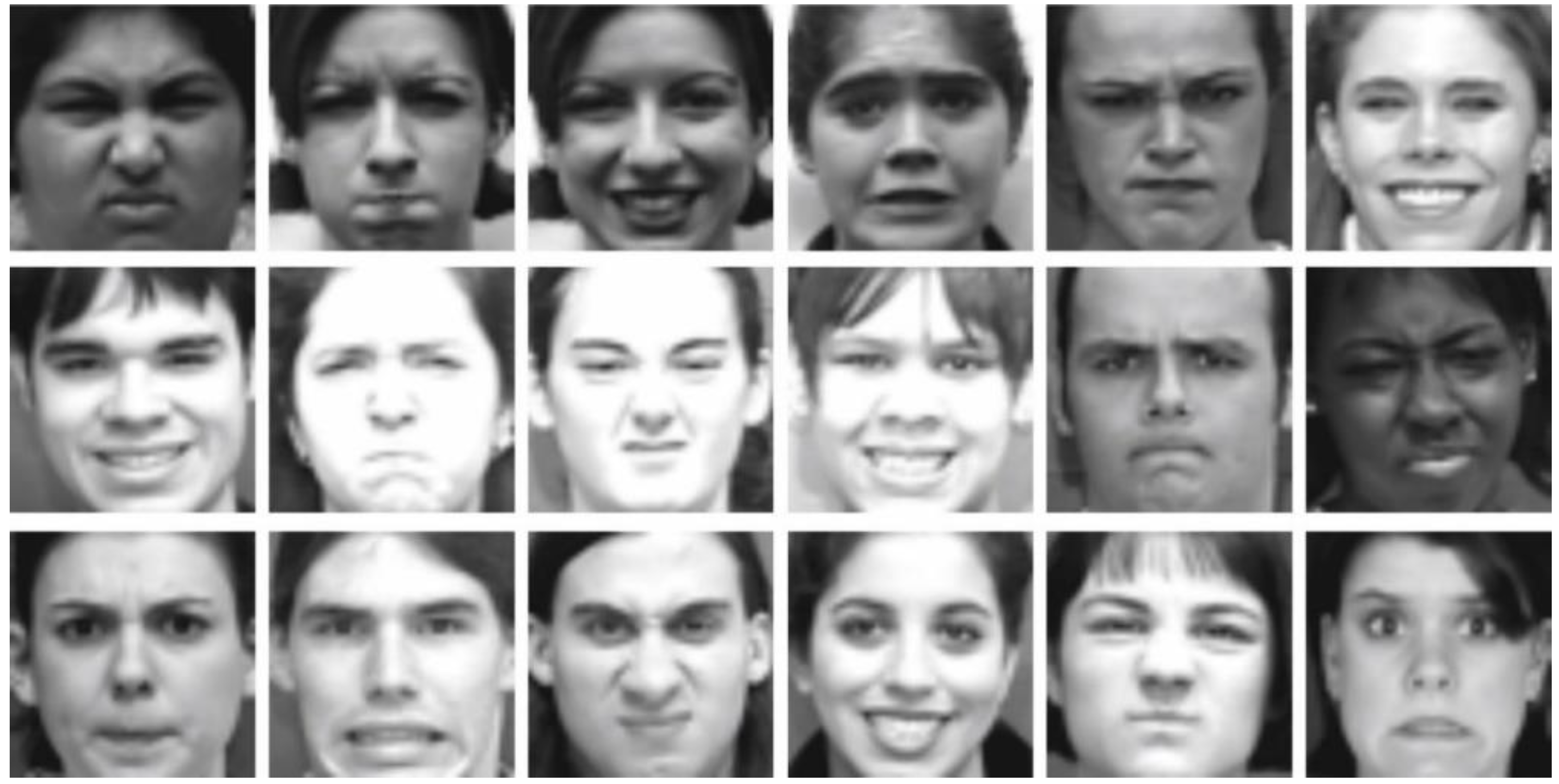
The experimental justification of the RFER-EADL technique took place using the CK+ dataset [26], which holds 837 images under seven class labels, as depicted in Table 2. Figure 4 shows some sample images. The FER-2013 dataset’s training set has 28,000 tagged images. The development set includes 3500 tagged photos, whereas the test set includes 3500 images. FER-2013 labels each image with one of seven emotions: joyful, sad, angry, terrified, astonished, disgusted, or neutral.
Happiness is the most prevalent emotion, being present in 24.4% of images. FER-2013 includes both posed and unposed headshots. The photos are all grayscale and 48 × 48 pixels in size. The FER-2013 dataset was created by compiling the results of each emotion’s Google search and its synonyms.
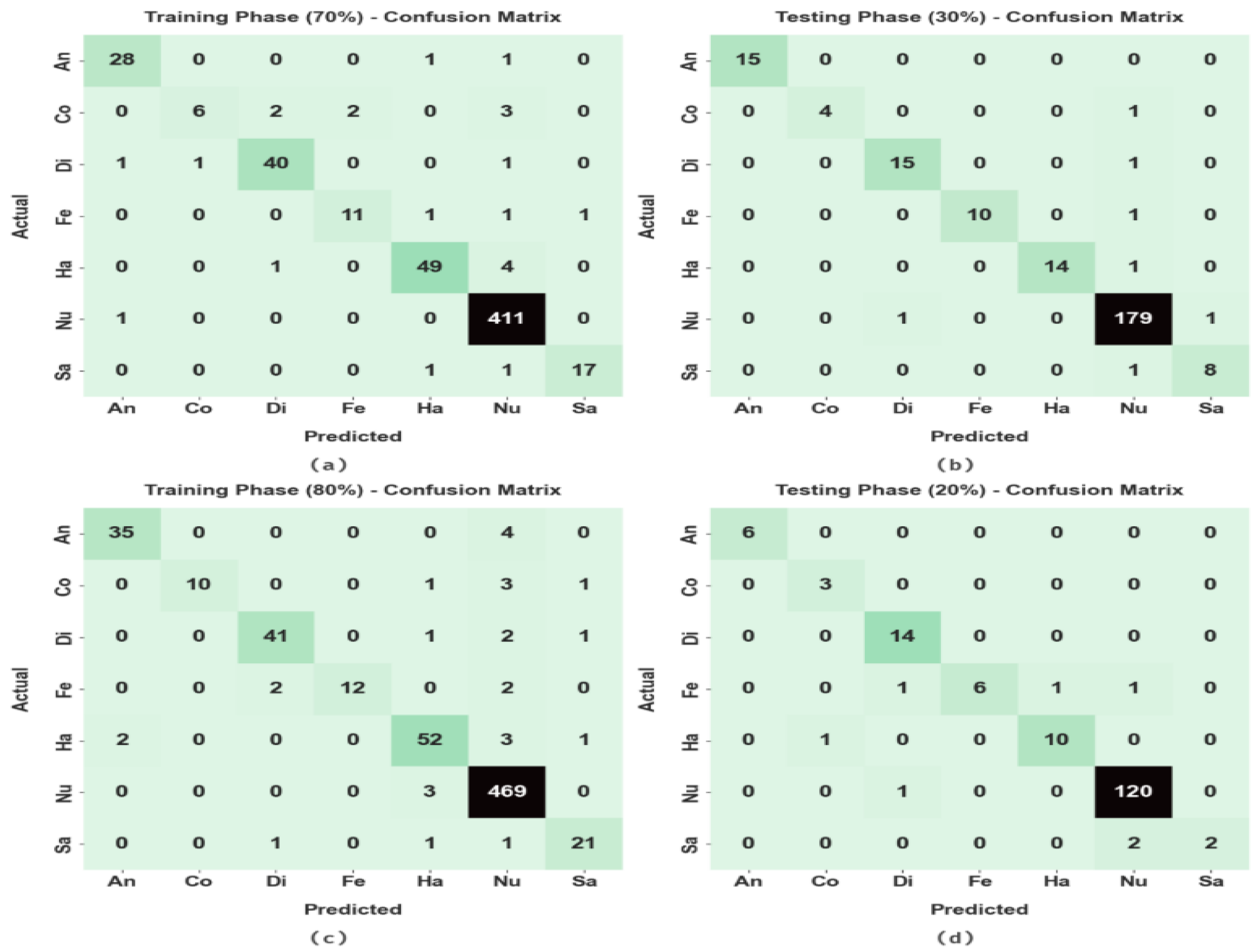
The RFER-EADL confusion matrices produced on the FER process are showcased in Figure 5. The figure indicates that the RFER-EADL model expertly recognized all seven different facial expressions under varying TR and TS data.
Table 3 demonstrates the overall FER outcomes of the RFER-EADL model on 70% of TR data and 30% of TS data.
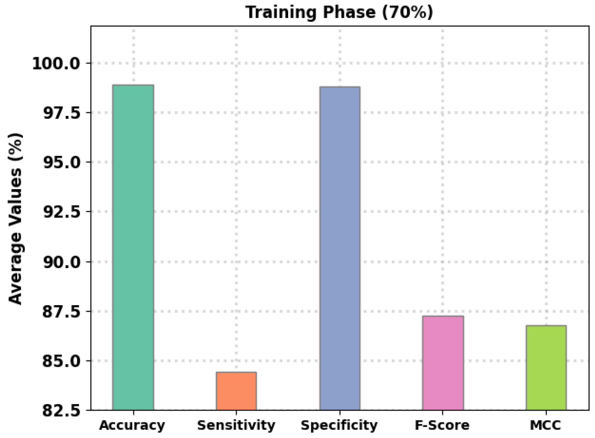
Figure 6 illustrates the FER results of the RFER-EADL model on 70% of the TR dataset. The results suggest that the RFER-EADL technique recognized all facial expressions accurately. For instance, in class A, the RFER-EADL model offered a c c u y of 99.32%, s e n s y of 93.33%, s p e c y of 99.64%, a n   F s c o r e of 93.33%, and an MCC of 92.97%. Additionally, for class Co, the RFER-EADL technique rendered a c c u y of 98.63%, s e n s y of 46.15%, s p e c y of 99.83%, an F s c o r e of 60%, and an MCC of 62.33%. Moreover, for class Di, the RFER-EADL technique granted a c c u y of 98.97%, s e n s y of 93.02%, s p e c y of 99.45%, an a c c u y of 93.02%, and an MCC of 92.47%.
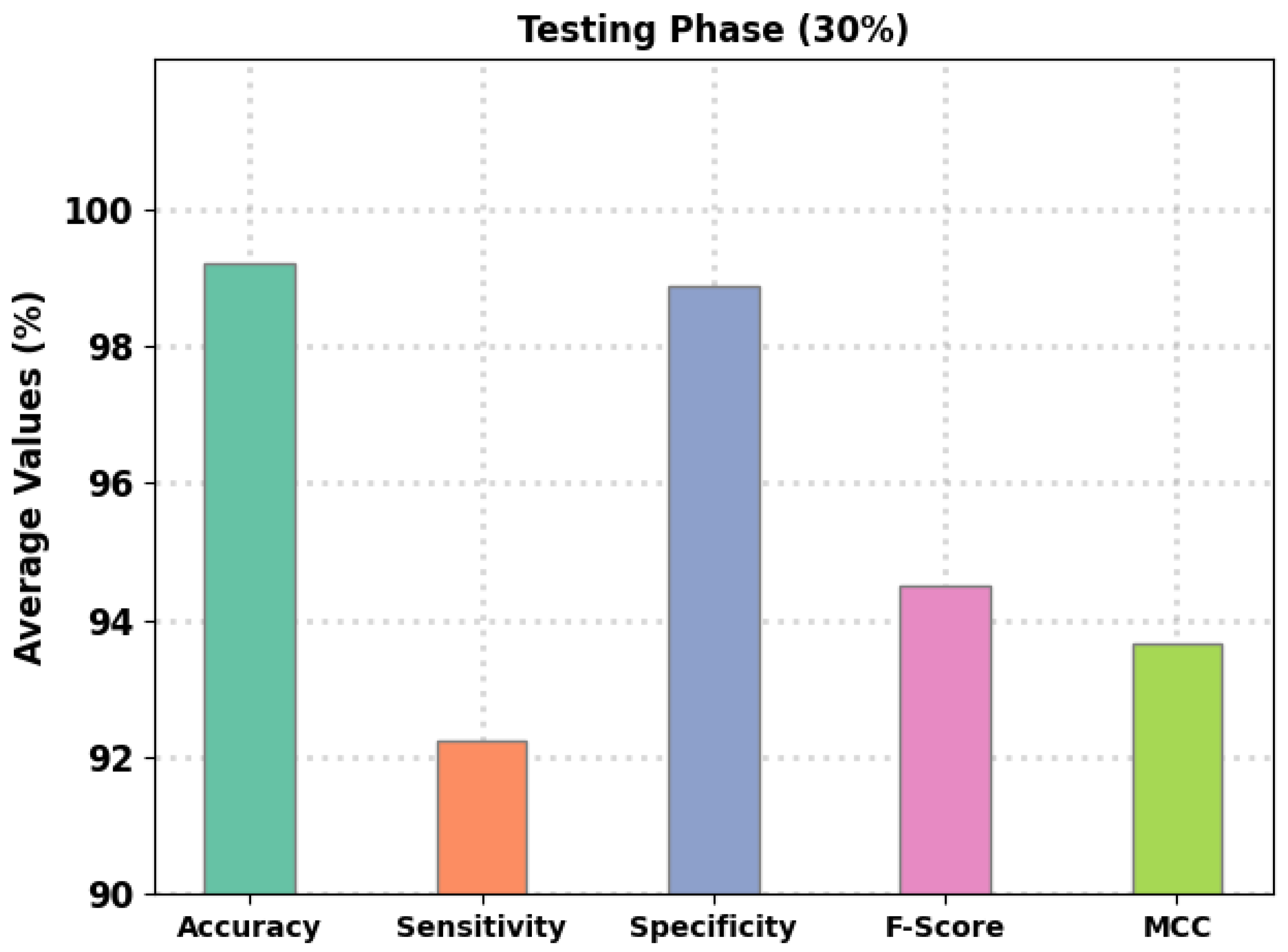
Figure 7 exemplifies the FER results of the RFER-EADL on 30% of the TS dataset. The outcomes denoted by the RFER-EADL approach recognized all facial expressions precisely. For example, for class A, the RFER-EADL technique achieved presented a c c u y of 100%, s e n s y of 100%, s p e c y of 100%, an F s c o r e of 100%, and an MCC of 100%. Likewise, for class Co, the RFER-EADL technique rendered a c c u y of 99.60%, s e n s y of 80%, s p e c y of 100%, an F s c o r e of 88.89%, and an MCC of 89.26%. Further, on class Di, the RFER-EADL technique provided a c c u y of 99.21%, s e n s y of 93.75%, s p e c y of 99.58%, an F s c o r e of 93.75%, and an MCC of 93.33%.
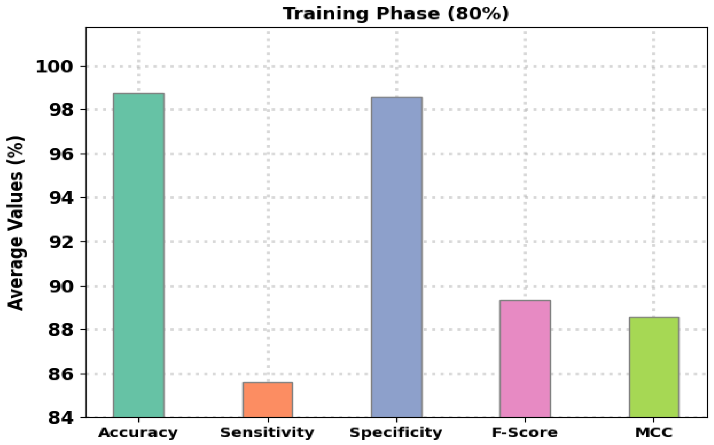
Table 4 establishes the overall FER results of the RFER-EADL approach on 20% of TS data and 80% of TR data. Figure 8 shows the FER results of the RFER-EADL technique on 80% of TR data. The effects specify that the RFER-EADL algorithm recognized all facial expressions accurately. For example, for class A, the RFER-EADL methodology provided a c c u y of 99.10%, s e n s y of 89.74%, s p e c y of 99.68%, an F s c o r e of 92.11%, and an MCC of 91.67%. Additionally, for class Di, the RFER-EADL approach provided a c c u y of 98.95%, s e n s y of 91.11%, s p e c y of 99.52%, an F s c o r e of 92.13%, and an MCC of 91.58%.
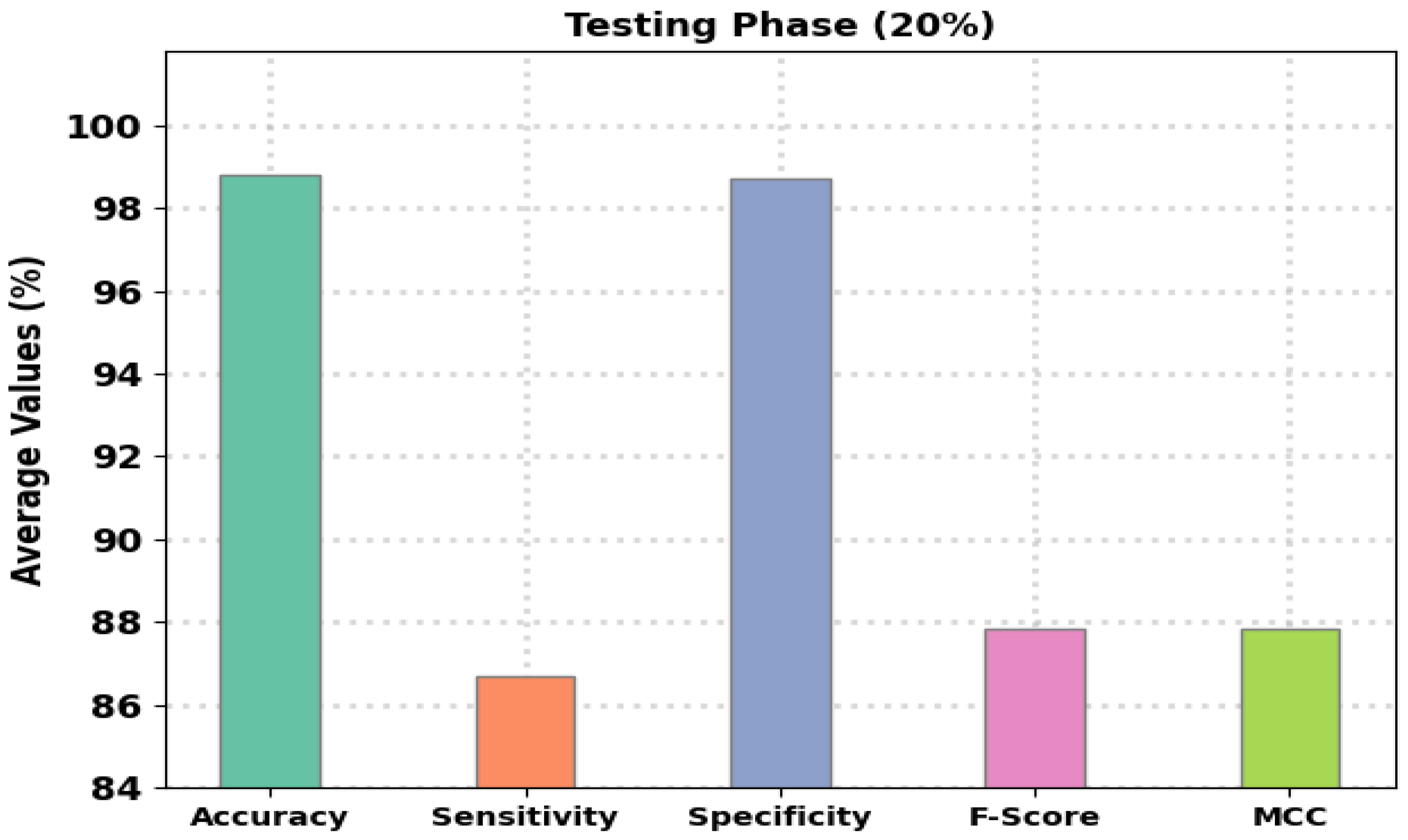
Figure 9 demonstrates the FER results of the RFER-EADL technique on 20% of the TS data. The results designate the RFER-EADL approach recognized all facial expressions accurately. For example, for class A, the RFER-EADL algorithm provided a c c u y of 100%, s e n s y of 100%, s p e c y of 100%, an F s c o r e of 100%, and an MCC of 100%. Additionally, for class Co, the RFER-EADL approach granted a c c u y of 99.40%, s e n s y of 100%, s p e c y of 99.39%, an F s c o r e of 85.71%, and an MCC of 86.34%. Additionally, for class Di, the RFER-EADL approach provided a c c u y of 98.81%, s e n s y of 100%, s p e c y of 98.70%, an F s c o r e of 93.33%, and an MCC of 92.93%.
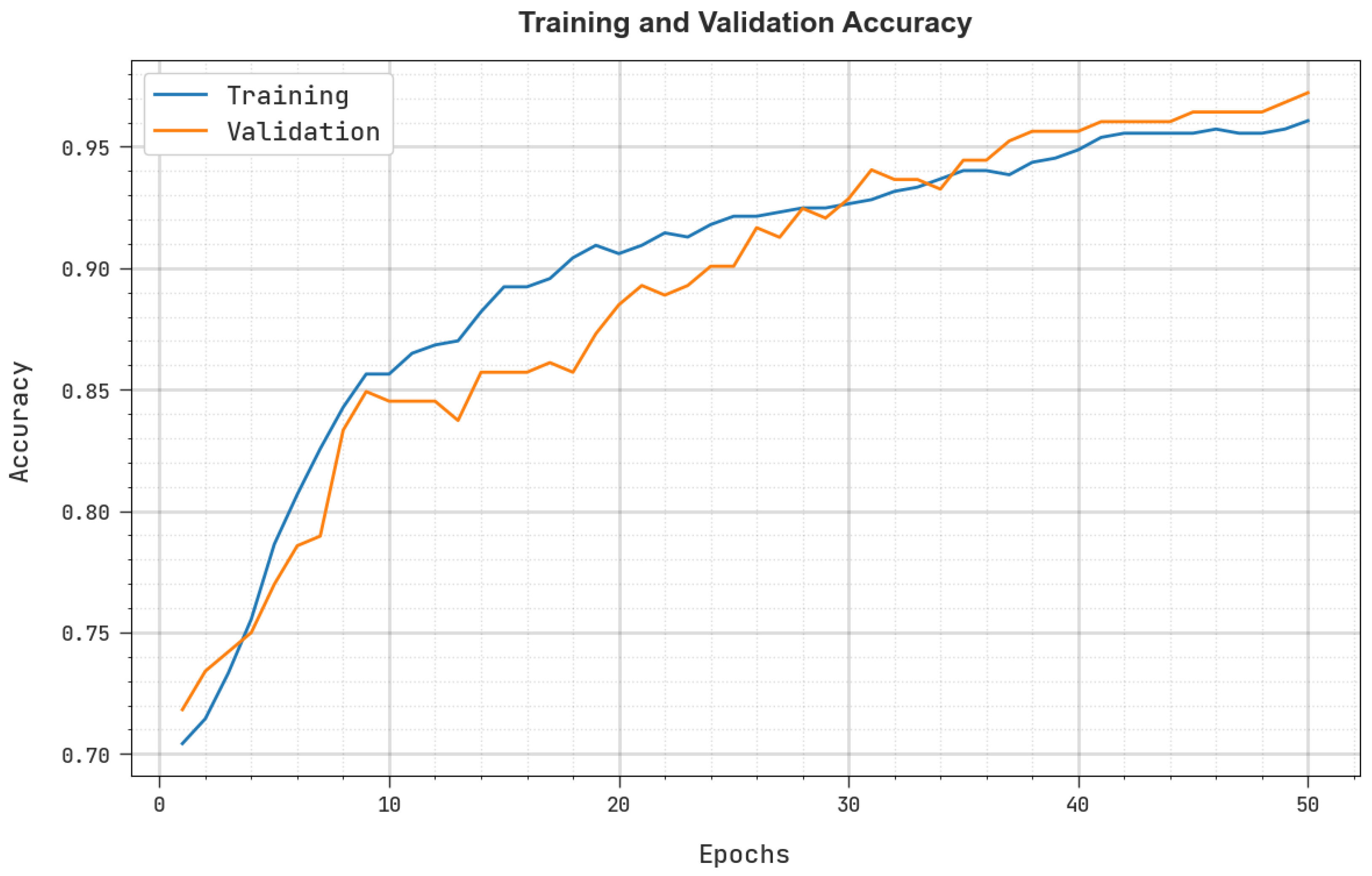
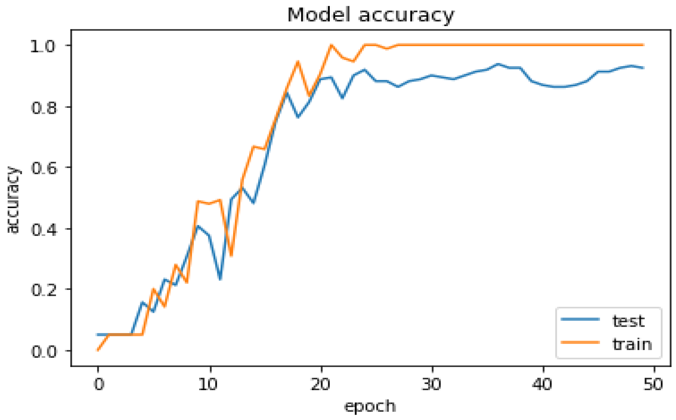
Figure 10 shows the training accuracy (TRA) and validation accuracy (VLA) obtained by the RFER-EADL approach on the test dataset. The experimental results show that the RFER-EADL approach obtained higher TRA and VLA values. VLA appears to be greater than TRA.
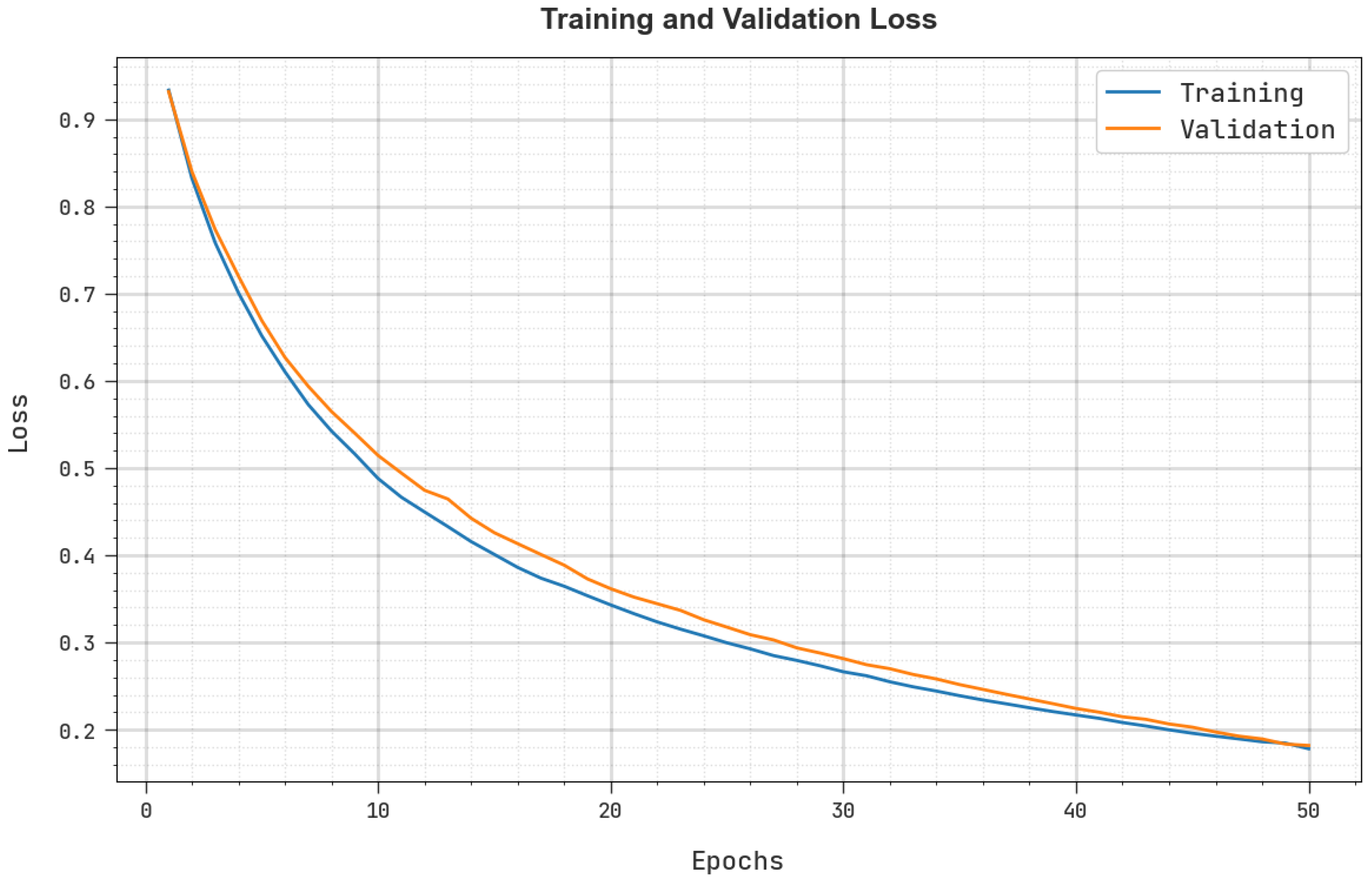
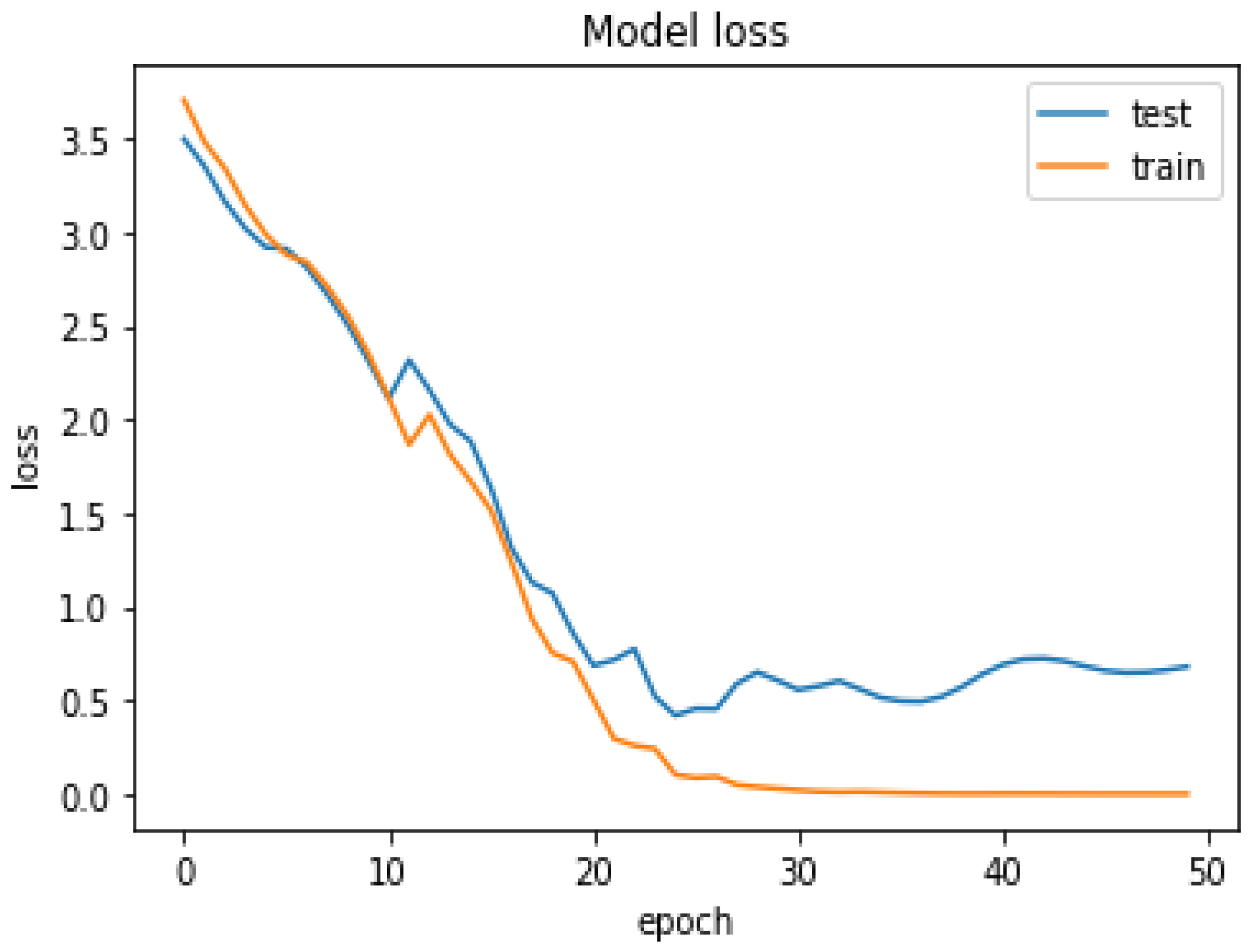
Figure 11 depicts the training loss (TRL) and validation loss (VLL) obtained by the RFER-EADL approach on the test dataset. The RFER-EADL approach produced experimental results with minimal TRL and VLL values. The VLL, in particular, is less than the TRL.
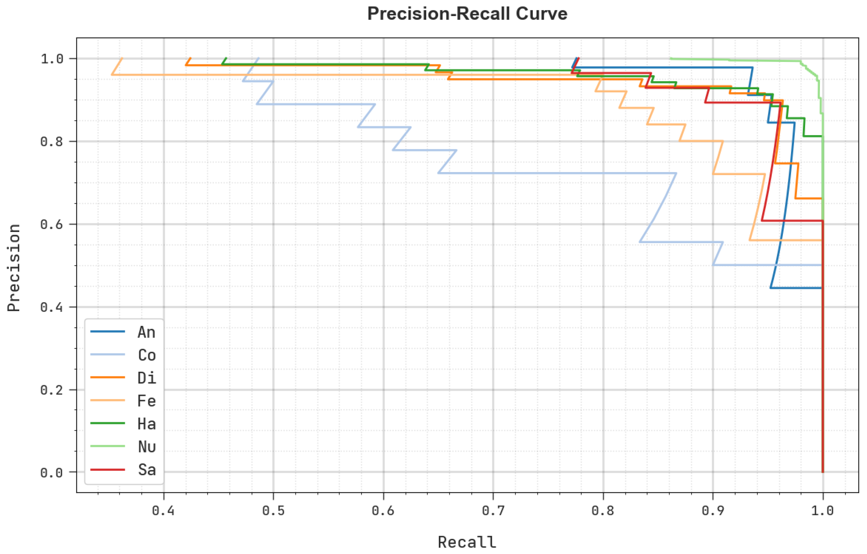
Figure 12 depicts a clear precision–recall assessment of the RFER-EADL algorithm using the test dataset. The RFER-EADL technique, as depicted in the figure, resulted in high precision–recall values in each class label.
Figure 13 depicts a quick ROC analysis of the RFER-EADL algorithm on the test dataset. The results demonstrate that the RFER-EADL approach is capable of classifying various classes.
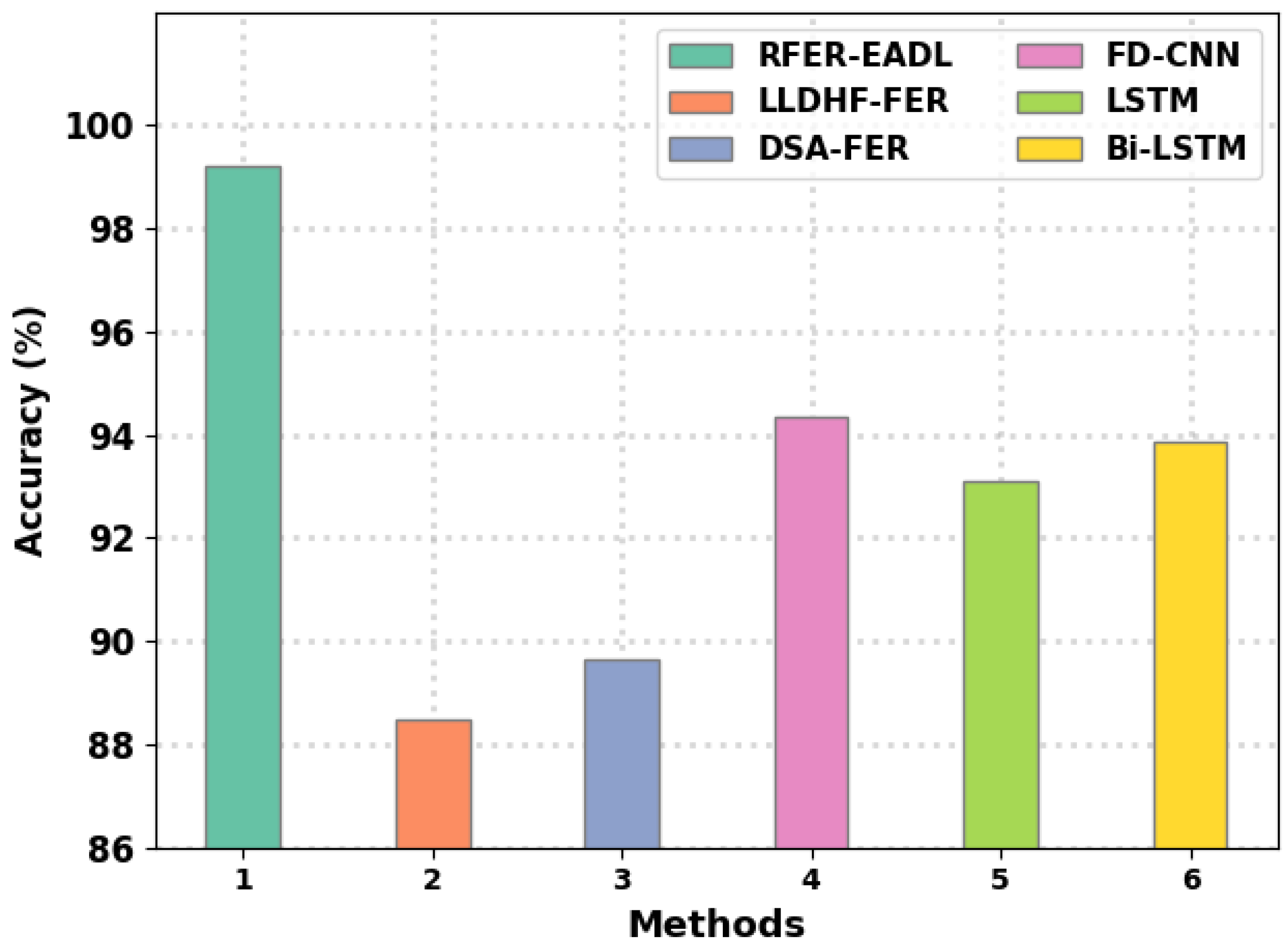
A comparison of the RFER-EADL model with other DL models is shown in Table 5 and Figure 14 [25]. These outcomes show that the LLDHF-FER and DSA-FER techniques reach lower a c c u y values of 88.49% and 89.64%, respectively.
Next, the LSTM and Bi-LSTM models reached closer a c c u y values of 93.12% and 93.87%, respectively. Though the FD-CNN model resulted in a considerable a c c u y of 94.35%, the RFER-EADL model provided the maximum a c c u y of 99.21%. These results confirm the enhanced FER outcomes of the RFER-EADL model.
Figure 15 displays the training and testing accuracy analysis of the RFER-EADL technique applied to localization data. In testing and training accuracy, the proposed RFER-EADL model achieved superior performance. Notable is the fact that after 50 epochs, the accuracy values become saturated. Testing accuracy becomes much smaller than the training accuracy after the 20th epochs. This means that our proposed model has higher performance in training and testing accuracy.
Figure 16 displays a validation loss analysis of the RFER-EADL technique applied to localization data. In comparison to training loss, the Faster RCNN-DBMF approach minimized loss values. Notable is the fact that after 50 epochs, the loss values become saturated. Training loss becomes much smaller than the validation loss after the 20th epochs. This means that our model has higher performance on the training dataset.

5. Conclusions

In this study, the RFER-EADL technique for emotion recognition in facial photographs was established. The RFER-EADL technique employs the HE process first. The COA with the DenseNet-169 model is then used to extract features. Finally, the TLBO with an LSTM model is used to identify and classify facial expressions. The COA and TLBO algorithms were designed to aid in the optimal parameter selection of the DenseNet and LSTM models, respectively. A brief simulation examination on the benchmark dataset showed that the RFER-EADL strategy outperforms alternatives. A thorough comparison analysis confirmed the RFER-EADL technique’s superiority over contemporary DL models. When compared to other conventional techniques, the RFER-EADL model outperformed them all, achieving the maximum accuracy of 99.21%. In the future, the RFER-EADL model could be used in real-time video surveillance applications.

Author Contributions

Conceptualization, M.A.V.R. and R.K.M.; methodology, N.S.; software, M.A.; validation, M.A.V.R., R.K.M. and N.S.; formal analysis, R.K.M.; investigation, N.S.; resources, N.S.; data curation, N.S.; writing—original draft preparation, M.A.V.R.; writing—review and editing, M.G.G. and N.S.; visualization, M.A.V.R.; supervision, R.K.M.; project administration, M.G.G. and M.A.V.R.; funding acquisition, N.S. All authors have read and agreed to the published version of the manuscript.

Funding

This research received no external funding.

Institutional Review Board Statement

Not applicable.

Informed Consent Statement

Not applicable.

Data Availability Statement

Data sharing not applicable.

Conflicts of Interest

The authors declare no conflict of interest.

References

  1. Fathima, A.; Vaidehi, K. Review on facial expression recognition system using machine learning techniques. In Advances in Decision Sciences, Image Processing, Security and Computer Vision; Springer: Cham, Switzerland, 2020; pp. 608–618. [Google Scholar]
  2. Ravichandran, T. An Efficient Resource Selection and Binding Model for Job Scheduling in Grid. Eur. J. Sci. Res. 2012, 81, 450–458. [Google Scholar]
  3. Revina, I.M.; Emmanuel, W.S. A survey on human face expression recognition techniques. J. King Saud Univ. Comput. Inf. Sci. 2021, 33, 619–628. [Google Scholar] [CrossRef]
  4. Mohan, P.; Thangavel, R. Resource Selection in Grid Environment based on Trust Evaluation using Feedback and Performance. Am. J. Appl. Sci. 2013, 10, 924–930. [Google Scholar] [CrossRef] [Green Version]
  5. Jaswanth, K.S.; David, D.S. A novel based 3D facial expression detection using recurrent neural network. In Proceedings of the 2020 International Conference on System, Computation, Automation and Networking (ICSCAN), Pondicherry, India, 3–4 July 2020; pp. 1–6. [Google Scholar]
  6. Jain, D.K.; Zhang, Z.; Huang, K. Multi angle optimal pattern-based deep learning for automatic facial expression recognition. Pattern Recognit. Lett. 2017, 139, 157–165. [Google Scholar] [CrossRef]
  7. Vo, T.-H.; Lee, G.-S.; Yang, H.-J.; Kim, S.-H. Pyramid With Super Resolution for In-the-Wild Facial Expression Recognition. IEEE Access 2020, 8, 131988–132001. [Google Scholar] [CrossRef]
  8. Zheng, H.; Wang, R.; Ji, W.; Zong, M.; Wong, W.K.; Lai, Z.; Lv, H. Discriminative deep multi-task learning for facial expression recognition. Inf. Sci. 2020, 533, 60–71. [Google Scholar] [CrossRef]
  9. Hardas, B.M.; Pokle, S.B. Optimization of Peak to Average Power Reduction in OFDM. J. Commun. Technol. Electron. 2017, 62, 1388–1395. [Google Scholar] [CrossRef]
  10. Hardas, B.M.; Pokle, S.B. Analysis of OFDM system using DCT-PTS-SLM based approach for multimedia applications. Clust. Comput. 2018, 22, 4561–4569. [Google Scholar] [CrossRef]
  11. Rajan, S.; Chenniappan, P.; Devaraj, S.; Madian, N. Novel deep learning model for facial expression recognition based on maximum boosted CNN and LSTM. IET Image Process. 2020, 14, 1373–1381. [Google Scholar] [CrossRef]
  12. Sikkandar, H.; Thiyagarajan, R. Deep learning based facial expression recognition using improved Cat Swarm Optimization. J. Ambient. Intell. Humaniz. Comput. 2020, 12, 3037–3053. [Google Scholar] [CrossRef]
  13. Wang, K.; Peng, X.; Yang, J.; Lu, S.; Qiao, Y. Suppressing uncertainties for large-scale facial expression recognition. In Proceedings of the IEEE/CVF Conference on Computer Vision and Pattern Recognition 2020, Seattle, WA, USA, 14–19 June 2020; pp. 6897–6906. [Google Scholar]
  14. Li, J.; Jin, K.; Zhou, D.; Kubota, N.; Ju, Z. Attention mechanism-based CNN for facial expression recognition. Neurocomputing 2020, 411, 340–350. [Google Scholar] [CrossRef]
  15. Cheng, S.; Zhou, G. Facial Expression Recognition Method Based on Improved VGG Convolutional Neural Network. Int. J. Pattern Recognit. Artif. Intell. 2019, 34, 2056003. [Google Scholar] [CrossRef]
  16. Cao, S.; Yao, Y.; An, G. E2-capsule neural networks for facial expression recognition using AU-aware attention. IET Image Process. 2020, 14, 2417–2424. [Google Scholar]
  17. Kim, J.-H.; Kima, B.-G.; Roy, P.P.; Jeong, D.-M. Efficient Facial Expression Recognition Algorithm Based on Hierarchical Deep Neural Network Structure. IEEE Access 2019, 7, 41273–41285. [Google Scholar] [CrossRef]
  18. Zhu, Q.; Mao, Q.; Jia, H.; Noi, O.E.N.; Tu, J. Convolutional relation network for facial expression recognition in the wild with few-shot learning. Expert Syst. Appl. 2021, 189, 116046. [Google Scholar] [CrossRef]
  19. Liu, S.; Gao, P.; Li, Y.; Fu, W.; Ding, W. Multi-modal fusion network with complementarity and importance for emotion recognition. Inf. Sci. 2023, 619, 679–694. [Google Scholar] [CrossRef]
  20. Liu, S.; Huang, S.; Fu, W.; Lin, J.C.-W. A descriptive human visual cognitive strategy using graph neural network for facial expression recognition. Int. J. Mach. Learn. Cybern. 2022, 1–17. [Google Scholar] [CrossRef]
  21. Mahmood, M.R.; Abdulrazaq, M.B.; Zeebaree, S.R.M.; Ibrahim, A.K.; Zebari, R.R.; Dino, H.I. Classification techniques’ performance evaluation for facial expression recognition. Indones. J. Electr. Eng. Comput. Sci. 2020, 21, 1176–1184. [Google Scholar] [CrossRef]
  22. Abdulrazaq, M.B.; Mahmood, M.R.; Zeebaree, S.R.M.; Abdulwahab, M.H.; Zebari, R.R.; Sallow, A.B. An Analytical Appraisal for Supervised Classifiers’ Performance on Facial Expression Recognition Based on Relief-F Feature Selection. J. Phys. Conf. Ser. 2021, 1804, 012055. [Google Scholar] [CrossRef]
  23. Rajaraman, P.V.; Prakash, M. Intelligent deep learning based bidirectional long short term memory model for automated reply of e-mail client prototype. Pattern Recognit. Lett. 2021, 152, 340–347. [Google Scholar] [CrossRef]
  24. Wu, M.; Su, W.; Chen, L.; Pedrycz, W.; Hirota, K. Two-Stage Fuzzy Fusion Based-Convolution Neural Network for Dynamic Emotion Recognition. IEEE Trans. Affect. Comput. 2020, 13, 805–817. [Google Scholar] [CrossRef]
  25. Neelakandan, S.; Paulraj, D.; Ezhumalai, P.; Prakash, M. A Deep Learning Modified Neural Network(DLMNN) based proficient sentiment analysis technique on Twitter data. J. Exp. Theor. Artif. Intell. 2022, 1–20. [Google Scholar] [CrossRef]
  26. Sunitha, G.; Geetha, K.; Neelakandan, S.; Pundir, A.K.S.; Hemalatha, S.; Kumar, V. Intelligent deep learning based ethnicity recognition and classification using facial images. Image Vis. Comput. 2022, 121, 104404. [Google Scholar] [CrossRef]
  27. Neelakandan, S.; Arun, A.; Bhukya, R.R.; Hardas, B.M.; Kumar, T.C.A.; Ashok, M. An Automated Word Embedding with Parameter Tuned Model for Web Crawling. Intell. Autom. Soft Comput. 2022, 32, 1617–1632. [Google Scholar] [CrossRef]
  28. Kavitha, M.; Babu, B.S.; Sumathy, B.; Jackulin, T.; Ramkumar, N.; Manimaran, A.; Walia, R.; Neelakandan, S. Convolutional Neural Networks Based Video Reconstruction and Computation in Digital Twins. Intell. Autom. Soft Comput. 2022, 34, 1571–1586. [Google Scholar] [CrossRef]
  29. Chandrasekaran, S.; Singh Pundir, A.K.; Lingaiah, T.B. Deep Learning Approaches for Cyberbullying Detection and Classification on Social Media. Comput. Intell. Neurosci. 2022, 2022, 2163458. [Google Scholar] [CrossRef]
  30. Bulut, F. Low dynamic range histogram equalization (LDR-HE) via quantized Haar wavelet transform. Vis. Comput. 2021, 38, 2239–2255. [Google Scholar] [CrossRef]
  31. Rahman, M.T.; Dola, A. Automated Grading of Diabetic Retinopathy using DenseNet-169 Architecture. In Proceedings of the 2021 5th International Conference on Electrical Information and Communication Technology (EICT), Khulna, Bangladesh, 17–19 December 2021; pp. 1–4. [Google Scholar]
  32. Jia, H.; Sun, K.; Zhang, W.; Leng, X. An enhanced chimp optimization algorithm for continuous optimization domains. Complex Intell. Syst. 2021, 8, 65–82. [Google Scholar] [CrossRef]
  33. Lei, J.; Liu, C.; Jiang, D. Fault diagnosis of wind turbine based on Long Short-term memory networks. Renew. Energy 2019, 133, 422–432. [Google Scholar] [CrossRef]
  34. Ashtiani, M.N.; Toopshekan, A.; Astaraei, F.R.; Yousefi, H.; Maleki, A. Techno-economic analysis of a grid-connected PV/battery system using the teaching-learning-based optimization algorithm. Sol. Energy 2020, 203, 69–82. [Google Scholar] [CrossRef]
  35. Available online: https://www.kaggle.com/datasets/shawon10/ckplus (accessed on 14 October 2022).
  36. Saeed, S.; Shah, A.A.; Ehsan, M.K.; Amirzada, M.R.; Mahmood, A.; Mezgebo, T. Automated Facial Expression Recognition Framework Using Deep Learning. J. Healthc. Eng. 2022, 2022, 5707930. [Google Scholar] [CrossRef] [PubMed]
  37. Farah Sayeed, R.; Princey, S.; Priyanka, S. Deployment of Multicloud Environment with Avoidance of DDOS Attack and Secured Data Privacy. Int. J. Appl. Eng. Res. 2015, 10, 8121–8124. [Google Scholar]
  38. Awari, H.; Subramani, N.; Janagaraj, A.; Thanammal, G.B.; Thangarasu, J.; Kohar, R. Three-dimensional dental image segmentation and classification using deep learning with tunicate swarm algorithm. Expert Syst. 2022, e13198. [Google Scholar] [CrossRef]
  39. Subbulakshmi, P.; Prakash, M.; Ramalakshmi, V. Honest Auction Based Spectrum Assignment and Exploiting Spectrum Sensing Data Falsification Attack Using Stochastic Game Theory in Wireless Cognitive Radio Network. Wirel. Pers. Commun. 2017, 102, 799–816. [Google Scholar] [CrossRef]
  40. Subbulakshmi, P.; Prakash, M. Mitigating eavesdropping by using fuzzy based MDPOP-Q learning approach and multilevel Stackelberg game theoretic approach in wireless CRN. Cogn. Syst. Res. 2018, 52, 853–861. [Google Scholar] [CrossRef]
  41. Mohan, P.; Sundaram, M.; Satpathy, S.; Das, S. An efficient technique for cloud storage using secured de-duplication algorithm. J. Intell. Fuzzy Syst. 2021, 41, 2969–2980. [Google Scholar] [CrossRef]
  42. Jain, D.K.; Liu, X.; Neelakandan, S.; Prakash, M. Modeling of human action recognition using hyperparameter tuned deep learning model. J. Electron. Imaging 2022, 32, 011211. [Google Scholar] [CrossRef]
  43. Prakash, P.R.; Anuradha, D.; Iqbal, J.; Galety, M.G.; Singh, R.; Neelakandan, S. A novel convolutional neural network with gated recurrent unit for automated speech emotion recognition and classification. J. Control Decis. 2022, 1–10. [Google Scholar] [CrossRef]
  44. Neelakandan, S.; Prakash, M.; Bhargava, S.; Mohan, K.; Robert, N.R.; Upadhye, S. Optimal Stacked Sparse Autoencoder Based Traffic Flow Prediction in Intelligent Transportation Systems. In Virtual and Augmented Reality for Automobile Industry: Innovation Vision and Applications; Springer: Cham, Switzerland, 2022; pp. 111–127. [Google Scholar] [CrossRef]
  45. Banu, J.F.; Neelakandan, S.; Geetha, B.; Selvalakshmi, V.; Umadevi, A.; Martinson, E.O. Artificial Intelligence Based Customer Churn Prediction Model for Business Markets. Comput. Intell. Neurosci. 2022, 2022, 1703696. [Google Scholar] [CrossRef]
  46. Neelakandan, S.; Prakash, M.; Geetha, B.; Nanda, A.K.; Metwally, A.M.; Santhamoorthy, M.; Gupta, M.S. Metaheuristics with Deep Transfer Learning Enabled Detection and classification model for industrial waste management. Chemosphere 2022, 308, 136046. [Google Scholar] [CrossRef]
  47. Sreekala, K.; Cyril, C.P.D.; Neelakandan, S.; Chandrasekaran, S.; Walia, R.; Martinson, E.O. Capsule Network-Based Deep Transfer Learning Model for Face Recognition. Wirel. Commun. Mob. Comput. 2022, 2022, 2086613. [Google Scholar] [CrossRef]
  48. Jain, D.K.; Neelakandan, S.; Veeramani, T.; Bhatia, S.; Memon, F.H. Design of fuzzy logic based energy management and traffic predictive model for cyber physical systems. Comput. Electr. Eng. 2022, 102, 108135. [Google Scholar] [CrossRef]
  49. Raghavendra, S.; Harshavardhan, A.; Neelakandan, S.; Partheepan, R.; Walia, R.; Rao, V.C.S. Multilayer Stacked Probabilistic Belief Network-Based Brain Tumor Segmentation and Classification. Int. J. Found. Comput. Sci. 2022, 33, 559–582. [Google Scholar] [CrossRef]
  50. Parthiban, S.; Harshavardhan, A.; Neelakandan, S.; Prashanthi, V.; Alolo, A.-R.A.A.; Velmurugan, S. Chaotic Salp Swarm Optimization-Based Energy-Aware VMP Technique for Cloud Data Centers. Comput. Intell. Neurosci. 2022, 2022, 4343476. [Google Scholar] [CrossRef]
  51. Jain, D.K.; Tyagi, S.K.S.; Neelakandan, S.; Prakash, M.; Natrayan, L. Metaheuristic Optimization-Based Resource Allocation Technique for Cybertwin-Driven 6G on IoE Environment. IEEE Trans. Ind. Inform. 2021, 18, 4884–4892. [Google Scholar] [CrossRef]
  52. Venu, D.; Mayuri, A.; Neelakandan, S.; Murthy, G.; Arulkumar, N.; Shelke, N. An efficient low complexity compression based optimal homomorphic encryption for secure fiber optic communication. Optik 2021, 252, 168545. [Google Scholar] [CrossRef]
  53. Lakshmanna, K.; Subramani, N.; Alotaibi, Y.; Alghamdi, S.; Khalafand, O.I.; Nanda, A.K. Improved Metaheuristic-Driven Energy-Aware Cluster-Based Routing Scheme for IoT-Assisted Wireless Sensor Networks. Sustainability 2022, 14, 7712. [Google Scholar] [CrossRef]
  54. Harshavardhan, A.; Boyapati, P.; Neelakandan, S.; Akeji, A.A.A.-R.; Pundir, A.K.S.; Walia, R. LSGDM with Biogeography-Based Optimization (BBO) Model for Healthcare Applications. J. Healthc. Eng. 2022, 2022, 2170839. [Google Scholar] [CrossRef]
  55. Le, T.T.Q.; Tran, T.K.; Rege, M. Dynamic image for micro-expression recognition on region-based framework. In Proceedings of the 2020 IEEE 21st International Conference on Information Reuse and Integration for Data Science (IRI), Las Vegas, NV, USA, 11–13 August 2020; pp. 75–81. [Google Scholar]
  56. Saravanakumar, C.; Priscilla, R.; Prabha, B.; Kavitha, A.; Prakash, M.; Arun, C. An Efficient On-Demand Virtual Machine Migration in Cloud Using Common Deployment Model. Comput. Syst. Sci. Eng. 2022, 42, 245–256. [Google Scholar] [CrossRef]
  57. Geetha, B.T.; Mohan, P.; Mayuri, A.V.R.; Jackulin, T.; Stalin, J.L.A.; Anitha, V. Pigeon Inspired Optimization with Encryption Based Secure Medical Image Management System. Comput. Intell. Neurosci. 2022, 2022, 2243827. [Google Scholar] [CrossRef]
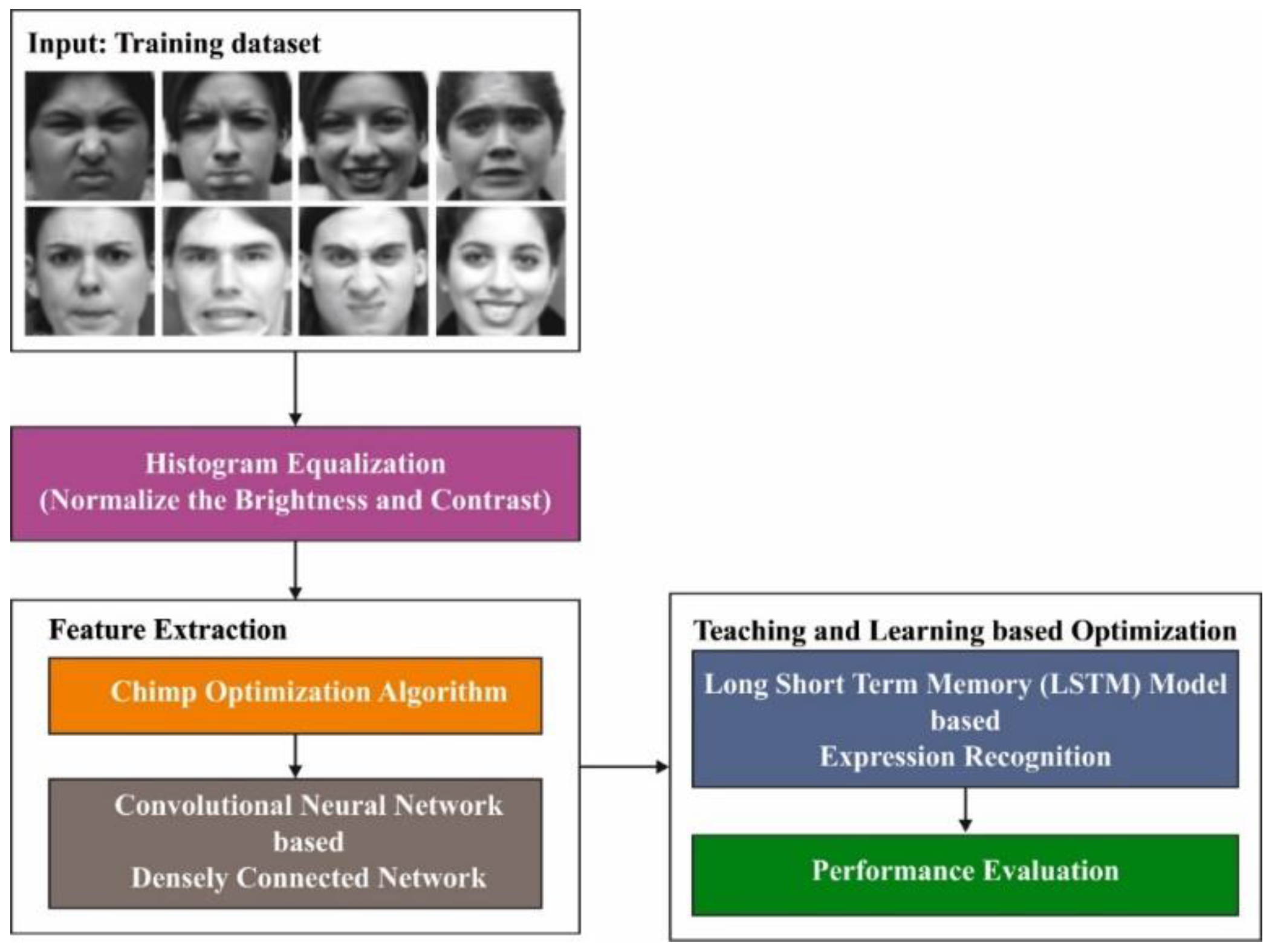
Figure 1. Block diagram of the RFER-EADL approach.
Applsci 13 00468 g001
Figure 2. Architecture of LSTM.
Applsci 13 00468 g002
Figure 3. RFER-EADL’s process.
Applsci 13 00468 g003
Figure 4. Sample images.
Applsci 13 00468 g004
Figure 5. Confusion matrices of the RFER-EADL algorithm: (a) 70% of the TR dataset, (b) 30% of the TS dataset, (c) 80% of the TR dataset, and (d) 20% of the TS dataset.
Applsci 13 00468 g005
Figure 6. Average analysis of the RFER-EADL algorithm under 70% of TR dataset.
Applsci 13 00468 g006
Figure 7. Average analysis of RFER-EADL algorithm under 30% of the TS dataset.
Applsci 13 00468 g007
Figure 8. Average analysis of the RFER-EADL algorithm for 80% of the TR dataset.
Applsci 13 00468 g008
Figure 9. Average analysis of the RFER-EADL algorithm for 20% of the TS dataset.
Applsci 13 00468 g009
Figure 10. TRA and VLA analysis of the RFER-EADL algorithm.
Applsci 13 00468 g010
Figure 11. TRL and VLL analysis of the RFER-EADL algorithm.
Applsci 13 00468 g011
Figure 12. Precision–recall analysis of the RFER-EADL algorithm.
Applsci 13 00468 g012
Figure 13. ROC curve analysis of the RFER-EADL algorithm.
Applsci 13 00468 g013
Figure 14. A c c u y analysis of the RFER-EADL approach and other modern algorithms.
Applsci 13 00468 g014
Figure 15. RFER-EADL training and testing accuracy.
Applsci 13 00468 g015
Figure 16. Proposed RFER-EADL model validation loss analysis.
Applsci 13 00468 g016
Table 1. Objectives and significant results of existing works.
Reference & YearObjectivesClassificationSignificant ResultsAccuracy Results
[20], 2021feature selection and classification methods for Facial Expression Recognition Support Vector Machine, Random Forest and KNN algorithmsBased on minimum chi-square features, achieved a consistency performance of many controlled classifiers to determine face expression.Achieved a 94.23% accuracy.
[21], 2021To propose effective classification Sequence of face and Expression collectionRandom forest, Decision Tree, SVM and KNN algorithmsReliever-F technique for function by focusing on the utilization of a small number of attributes.Achieved a 94.93% accuracy.
[22], 2021To propose efficient modality fusionFuzzy Fusion based neural networksImbalanced emotion recognition is handled by TSFFCNNAchieved eNTERFACE’ 05 90.82%
[23], 2020To improve the spontaneous detection of facial micro-expressions by sophisticated hand extraction model.Convolutional Neural Networks algorithmsSimple methods and effective classification for micro expression Achieved 67.3% for SMIC dataset, Achieved 66.67% SAMM dataset
Table 2. Dataset details.
LabelDescriptionNo. of Images
AnAnger45
CoContempt18
DiDisgust59
FeFear25
HaHappy69
NuNeutral593
SaSad28
Total Number of Images837
Table 3. RFER-EADL algorithm with different class labels for 70:30 of TR and TS datasets.
LabelsAccuracySensitivitySpecificityF-ScoreMCC
Training Validation (70%)
An99.3293.3399.6493.3392.97
Co98.6346.1599.8360.0062.33
Di98.9793.0299.4593.0292.47
Fe99.1578.5799.6581.4881.10
Ha98.6390.7499.4492.4591.72
Nu97.9599.7693.6498.5695.07
Sa99.4989.4799.8291.8991.66
Average98.8884.4498.7887.2586.76
Testing (30%)
An100.00100.00100.00100.00100.00
Co99.6080.00100.0088.8989.26
Di99.2193.7599.5893.7593.33
Fe99.6090.91100.0095.2495.15
Ha99.6093.33100.0096.5596.41
Nu97.2298.9092.9698.0893.09
Sa99.2188.8999.5988.8988.48
Average99.2192.2598.8794.4993.67
Table 4. Results of the RFER-EADL algorithm for 80:20 of the TR and TS datasets.
LabelsAccuracySensitivitySpecificityF-ScoreMCC
Training Phase (80%)
An99.1089.7499.6892.1191.67
Co99.2566.67100.0080.0081.34
Di98.9591.1199.5292.1391.58
Fe99.4075.00100.0085.7186.34
Ha98.2189.6699.0289.6688.67
Nu97.3199.3692.3998.1293.50
Sa99.1087.5099.5387.5087.03
Average98.7685.5898.5989.3288.59
Testing Phase (20%)
An100.00100.00100.00100.00100.00
Co99.40100.0099.3985.7186.34
Di98.81100.0098.7093.3392.93
Fe98.2166.67100.0080.0080.89
Ha98.8190.9199.3690.9190.27
Nu97.6299.1793.6298.3694.06
Sa98.8150.00100.0066.6770.28
Average98.8186.6898.7387.8587.82
Table 5. Comparative analysis of RFER-EADL and other modern algorithms.
MethodsAccuracy (%)
RFER-EADL99.21
LLDHF-FER88.49
DSA-FER89.64
FD-CNN94.35
LSTM93.12
Bi-LSTM93.87
Disclaimer/Publisher’s Note: The statements, opinions and data contained in all publications are solely those of the individual author(s) and contributor(s) and not of MDPI and/or the editor(s). MDPI and/or the editor(s) disclaim responsibility for any injury to people or property resulting from any ideas, methods, instructions or products referred to in the content.