Abstract
The scheduled maintenance cost of warships is the essential prerequisite and economic foundation to guarantee the effective implementation of maintenance, which directly influences the quality and efficiency of maintenance operations. This paper proposes a multi-target regression algorithm based on multi-layer sparse structure (MTR-MLS) algorithm, to achieve simultaneous prediction of the subentry costs of warship scheduled maintenance, and the total cost of the maintenance is estimated by summing the predicted values of the different subentry costs. In MTR-MLS, the kernel technique is employed to map the inputs to the higher dimensional space for decoupling the complex input–output nonlinear relationships. By deploying the structure matrix, MTR-MLS achieves a latent variable model which can explicitly encode the inter-target correlations via l2,1-norm-based sparse learning. Meanwhile, the noises are encoded to diminish the influence of noises while exploiting the correlations among targets. An alternating optimization algorithm is proposed to solve the objective function. Extensive experimental evaluation on real-world datasets and datasets of warships scheduled maintenance cost show that the proposed method consistently outperforms the state-of-the-art algorithms, which demonstrates its great effectiveness for cost prediction of warships scheduled maintenance.
1. Introduction
The warships scheduled maintenance (WSM) refers to the preventive repairment that is carried out by comprehensively considering the combat readiness and training tasks of the ship equipment, as well as the protective performance of the ship hull, the main equipment technical status and other related factors. Since the WSM costs constitute a large proportion of the total life cycle costs of warships, the cost prediction of WSM naturally becomes an important research topic in guaranteeing naval equipment maintenance [1].
Due to the complexity of cost-driving factors and the difficulty of obtaining the cost variation knowledge with small data size, existing studies mainly use methods such as grey prediction [2,3,4,5,6,7], case-based reasoning [8,9,10,11,12,13], support vector regression (SVR) [14,15,16,17] and so on, to model and predict cost in different fields. However, the above methods such as grey prediction and SVR are often based on a single output structure when predicting the costs, and output results are single-dimensional, which does not take advantage of the correlation information between different WSM subentry costs. The total costs of WSM can be further subdivided into subentry costs such as material costs, labour costs, manufacturing costs, etc. There is a strong correlation between different subentry costs. However, the grey prediction or SVR can only be used as a univariate modelling technique due to its inherent single-output structure. Consequently, the cost prediction model based on grey theory or SVR constructs a different predicted engine for each subentry cost separately, which ignores the inherent information of the mutual relationships among different subentry costs, which may lead to a poor prediction performance of the total costs.
With the burgeoning development of the neural network, different cost prediction models based on the neural network have been proposed [18,19,20,21,22]. Different types of artificial neural networks (ANN), such as back propagation neural networks (BPNN) [23], radial basis function neural networks (RBFNN) [20], and deep convolutional neural networks (DCNN) [19] are effective in cost prediction for different projects. Although the neural network has a multi-dimensional output structure, it is prone to underfitting or overfitting in the case of a small size of samples, which also leads to poor performance in the cost prediction of small samples. Moreover, the training of neural networks is vulnerable to anomalous samples and noise, which restrict their application in the cost prediction of WSM problems.
Multi-target regression (MTR) is the prediction of multiple continuous variables by a set of common input variables [24]. MTR not only exploits the correlation between input and output variables but also explores the correlation information between different output targets so that it can obtain better prediction performance than single-output regression when predicting multiple correlated variables. In this paper, the MTR algorithm based on multi-layer sparse structure (MTR-MLS) is proposed to model and predict the subentry costs of WSM simultaneously. The multi-output structure of the proposed algorithm is utilized to achieve accurate subentry costs prediction. Furthermore, the total cost of WSM is obtained by summing up the predicted subentry costs, which can efficiently improve the prediction accuracy and stability of WSM cost. The contributions of this paper are summarized as follows:
- Based on the traditional MTR framework, the latent variable space is introduced to form a multi-layer learning structure, and the sparsity constraint is imposed so that the same latent variables can be shared among the associated targets, thus improving the performance of the algorithm with multiple outputs.
- An auxiliary matrix is introduced in the latent variable space to learn the structural noise among the output targets and reduce its adverse effects on the regression modelling, and an alternating optimization algorithm is proposed for solving the problem.
- The MTR algorithm is applied to the WSM cost prediction problem to improve the prediction accuracy of subentry costs and total costs by making use of the correlation information among different subentry costs. Extensive experimental evaluation on real-world datasets and cost datasets of WSM demonstrate the effectiveness of the proposed method in the WSM cost prediction problem.
2. Related Work
2.1. Warships Scheduled Maintenance Cost Prediction
The category of warships maintenance is divided into condition-based preventive maintenance, temporary emergency maintenance and scheduled maintenance. The warships scheduled maintenance can also be divided into different grades according to their scope and depth, such as third-grade maintenance, second-grade, and first-grade maintenance.
Depending on the mission of the warships, the structure of warships’ scheduled maintenance during their whole life cycle varies. The structural diagram of a general warship’s scheduled maintenance is shown in Figure 1. During the service period, the warship will undergo several rounds of scheduled maintenance, and the times of scheduled maintenance occur differently for different grades, such as the highest grade of first-grade maintenance is often performed only once in the middle of its commissioning. The higher the maintenance grade, the less time occurs, and the greater the scope and depth of the grade maintenance. The timing of the different scheduled maintenance is relatively fixed, and their corresponding repair times are also determined.
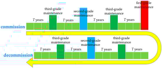
Figure 1.
Structural diagram of WSM during service life.
The WSM is a massive and complicated project that involves numerous different systems of the warship, such as the piping system, power system, etc. Moreover, the inter-coupling and complex relationships between maintenance tasks of different systems lead to less quantifiable maintenance information among them. This also makes it difficult to deconstruct the structure of the WSM work; traditional cost forecasting methods based on engineering decomposition have difficulty in achieving satisfactory results. Furthermore, its corresponding data collection also incurs significant labour and time costs.
Consequently, the primary ideology of WSM cost prediction is to establish the regression model by selecting relevant quantifiable feature indicators from the basic information and the corresponding maintenance scenarios of warships, with cost indicators as the output target. The regression model is employed to investigate statistical dependences between input features and costs, and then to estimate WSM costs based on the dependences. As the number of samples increases, these parametric models become more flexible and adaptive, accurate, and reliable, and they can also achieve significant reductions in time in terms of data collection.
Given the small sample size of WSM data, various grey prediction models were introduced to perform cost forecasting such as GM(0, N) [6], GM(1, 1) [4] and grey correlation analysis [2] to construct the time-series model for short-term forecasting of WMS maintenance costs. The GM(0, N) warship maintenance cost prediction model based on the priority accumulation method of similar information is proposed in [6], to solve the warship maintenance cost prediction problem in the small sample case. In [5], the grey orthogonal method is proposed to analyze the influencing factors of the naval vessel maintenance cost, and further determine the major and minor influencing factors of maintenance cost. The combined prediction model for warship maintenance cost measurement based on grey correlation ranking was developed in [3].
As an emerging field in artificial intelligence, with its historical experience-based solution mechanism, case-based reasoning (CBR) is well suited to the problem of WSM cost prediction, which has difficulty determining an explicit model and lacks abundant experience, therefore, various CBR-based WSM cost prediction methods have been proposed [1,8,9,10,11,12]. The literature [8] proposes a similarity retrieval technique and case adaptation technique for WMS cost cases based on CBR so that it can better adapt to the characteristics of WMS cases. Through an active learning strategy, a corresponding maintenance cost case library is formed, which in turn ensures the prediction accuracy of CBR technology on WMS costs. The literature [11] proposes a CBR system for WMS maintenance cost based on a dual similarity retrieval strategy, to better select similar historical cases to construct a case adaptation model for prediction, and achieve better prediction results in the WMS cost prediction problem.
Although the above-mentioned cost prediction model has solved the WMS cost estimation problem to a degree, there are still some unresolved problems. These methods only perform regression modelling and prediction for the total cost of WMS, they do not utilize the information of subentry costs in original data, and the correlation information contained in different subentry costs is not explored, which limits the accuracy of the prediction model. Meanwhile, while the above model can be trained and learn from small samples with some generalization abilities, it is also susceptible to the influence of abnormal samples and noises.
2.2. MTR Algorithm
The existing MTR algorithms can be broadly classified into two categories: problem transformation methods and algorithm adaptation methods [24]. The former is to split the MTR problem into several single-target regression subproblems and solve them independently. The main drawback is that when predicting a single objective independently, the dependency relationship between different objectives is neglected, which affects the overall prediction performance. Therefore, in order to overcome these drawbacks, existing problem transformation methods such as stacked single-target (SST) borrow the idea of stacked generalization in multi-label classification to stack the prediction results of single-target regression [25]; random linear target combination (RLC) constructs new target variables by random linear combination of targets to improve the regression performance of the model when there are dependencies between targets [26]; ensemble of regressor chains (ERC) is based on the idea of classifier chains in multi-label learning, by constructing random target chains, linking single target models to make predictions in turn, and solving the chain order sensitivity problem by integration [25]. Although the above problem transformation methods perform well in some cases, their performance often depends on the chosen regression algorithm, and the complexity of the training process also causes a large computational cost when the data output is of high dimensionality or large size.
Unlike the problem transformation approach, the basic idea of algorithm adaptation is to construct a structured model that predicts all outputs simultaneously, and the correlation between inputs and outputs as well as the correlation between different targets can be handled in a single framework so that the model can consider the effects of both factors during the learning process. Most of the existing algorithmic adaptation methods explore the inter-target correlations by imposing corresponding regularization constraints on the regression coefficient matrix, which are often limited to the linear regression case. By assuming a priori knowledge of the output structure, constraints such as low rank, sparsity or streamlining are imposed on the corresponding coefficient matrices [27]. However, these linear models cannot handle complex nonlinear input–output relationships, and the above prior knowledge assumptions are often only effective in domain-specific problems, which cannot automatically and adaptively extract correlation knowledge from datasets in different domains, resulting in a lack of model adaptability.
In recent years, various nonlinear based algorithms have been proposed to better handle the nonlinear correlation between input and output in data. In the literature [28,29,30,31], kernel methods are introduced to the MTR problem to decouple the highly complex nonlinear input–output relationships. In [31], a learning output kernels (OKL) algorithm is proposed to reveal the complex correlation structure in the output space through kernel methods to improve the learning performance of the algorithm. In [32], the coefficient matrix in multitask regression is reshaped into a vector to explore the correlation between task goals, which not only fails to distinguish the correlation between task goals and intra-task correlation, but also ignores the negative correlation between goals. However, the covariance matrix needs to satisfy the a priori assumption that the matrix variables obey normal distribution. In [33], the covariance structure of the potential model parameters and the conditional covariance structure between the outputs are learned from the data so that the algorithm does not require the corresponding a priori knowledge. In the literature [27], a multi-layer multi-target regression (MMR) algorithm is proposed by combining robust low-rank learning methods and kernel methods. MMR takes advantage of the kernel approach of nonlinear feature learning and the structure of multilayer learning in latent variable space, while modeling the intrinsic target correlations and nonlinear input–output relationships, and explicitly encodes the correlations between targets using the structure matrix, providing a flexible and general multilayer learning paradigm for the field of multi-target regression. The Multi-Target Sparse Latent Regression (MSLR) algorithm proposed in [34] has a similar structure to MMR and achieves explicit sparse learning of inter-target correlations by imposing regularization constraints on the structure matrix.
Most of the existing MTR algorithms focus on exploring and mining the correlation among targets to improve the regression performance of different outputs simultaneously. Compared with the problem transformation method, the family of algorithm adaptation methods can well encode the correlation of targets to be easily interpreted. However, MTR modelling based on a single framework is often affected by noises, and it is often difficult to effectively extract the dependencies between different subentry costs of WSM for existing algorithm adaptation methods. Based on this, this paper proposes the corresponding MTR algorithm, while explicitly coding and learning the structured noises among the outputs in the latent variable layer, in order to better solve the problem of handling the structured noises in MTR.
3. MTR Algorithm Based on Multi-Layer Sparse Structure
3.1. Multi-Layer MTR
The purpose of MTR is to learn a mapping function to map the input space to the output space , d and Q are the dimensionality of input and output spaces, respectively. Without loss of generality, take the basic linear MTR model as an example, which can be expressed as , where is the multi-variate targets, is the input, and is the coefficient matrix corresponding to the model, which reflects the linear correlation between the input features and the output target. is the parameter vector corresponding to the target output , and is the bias. Given the training set , the following penalty objective function can be established:
where is the loss function and , and , N is the number of training samples and λ is the penalty parameter corresponding to coefficient matrix W. is the Frobenius norm of matrix of W, which can be computed by W, and is the regularization parameter. Equation (1) is a straightforward form of single-output linear ridge regression extended to multiple outputs. Although it can realize the optimization of multiple outputs simultaneously, it does not consider the correlation between different subentry cost variables in WSM data, and thus cannot explore the correlation knowledge in the original information of different subentry costs to improve the overall fitting performance of the model.
To effectively explore the intrinsic correlation of different subentry costs on WSM data, the latent variable space is introduced to form the corresponding multi-layer structure based on Equation (1). Compared with the traditional method of applying various constraints to the coefficient matrix W to explore the correlation between target outputs, the multi-layer multi-output structure based on latent variable space can effectively separate the redundant relationship between feature inputs and structural correlation between outputs, which makes the learned coefficient matrix more interpretable and flexible. On the other hand, the multi-layer multi-output structure is more conducive to decoupling and expressing the complex input–output relationships in high-dimensional data. By sparse coding of inter-target correlations in the latent variable space, the correlations among WSM subentry costs can be better explored and expressed. The MTR model is constructed as follows:
where , and contains the latent variables in the latent space, is the structure matrix designed to explore correlations between different targets. The -norm regularization constraints on the structure matrix S encourage the correlated targets to share similar parameter sparsity patterns to capture a common set of features, i.e., latent variables in the latent space. Unlike the literature [31,33,35] where the coefficient matrix is solved based on prior assumption of normal distribution, the structural matrix S in Equation (2) is learned in a data-driven manner, which does not rely on any a prior assumption of the correlation between different target outputs in mining the correlation between targets, and thus is more flexible and adaptable. However, Equation (2) is still unable to handle complex nonlinear input–output relations, so the kernel trick is introduced to extend it.
3.2. Non-Linear Extensions Based on Kernel Tricks
In order to improve the fitting ability of the multi-layer MTR model in the nonlinear case, the kernel technique is introduced to extend it. Based on the Representer Theorem [36], the linear learner can be extended to a nonlinear learner by kernelization in the Reproducing Kernel Hilbert Space (RKHS). Denoting the regression coefficient matrix W as the combination of mappings of input samples in , we have , where is the coefficient matrix. Rewrite Equation (2) in trace form:
where α is the penalty parameter and is the diagonal matrix, and
in which is the i-th column of S. In order to avoid division by zero, we further regularize according to the following equation,
where is a small constant. Equation (6) is approximately equivalent to Equation (5) when . We map the input data into the high-dimensional Hilbert space by the nonlinear mapping function , and the associated kernel function is . According to the Representer Theorem, the regression matrix can be represented by , where . Substituting it into Equation (4), we can obtain the following objective function:
Note that the bias b is omitted, since it can be absorbed into W by adding additional dimension into the input X. Define to be the kernel matrix in . Then, Equation (6) can be simplified:
The above equation provides a learning framework for multi-target sparse kernel regression based on latent variables. The multi-layer multi-output structure formed by introducing the space of latent variables can decompose the original regression coefficient matrix into a new coefficient matrix A and a structure matrix S, and the coefficient matrix A is utilized to explore the correlation information between inputs and outputs, and the structure matrix S is employed to represent the correlation among targets sparsely. Based on the framework of multi-target sparse kernel regression, the regularization constraints on the coefficient matrix can decouple the redundant correlations between different input features; and the regularization constraints on the structure matrix can reveal the correlation structure between targets. Moreover, different types of kernel functions can handle linear or nonlinear input–output relationships flexibly. However, when the noise level is high, this learning framework often has difficulty accurately representing the correlation between different target outputs.
3.3. Robust MTR by Alleviating Noises
Since the learning of relationships between output targets in MTR models is affected by some potential structured noises, when there is a strong correlation between different targets, the structured noise affects the modelling of the relationship between multiple output variables. Although these noises do not interfere with the correlation modelling between feature inputs and different output targets, they can interfere with the mining of correlation information between targets and lead to some bias in the correlation learning between target outputs. Therefore, considering the undesirable effects of structured noises, the sensitivity of the regression model is reduced by learning the structured noises in order to explore the correlation knowledge more accurately. First, an auxiliary matrix is introduced in the latent variable space to explicitly encode the potential structured noises, which results in the following output structure:
where F is an unobserved latent feature matrix used to capture the structured noises in the latent space. By imposing the corresponding sparse regularization constraint on F and kernelizing the structure of Equation (8) into Equation (7), we obtain the final multi-layer MTR model considering structured noise as follows:
where, λ1, λ2, λ3 are the non-negative regularization parameters corresponding to the different regularization constraints. By introducing the learning of structured noises to improve the robustness of the model and weaken the adverse effects of structured noises on the algorithm, to explore the complex correlations more accurately among the multi-target outputs. The final objective function of MTR algorithm based on multi-layer sparse structure (MTR-MLS) is shown in Figure 2.
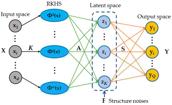
Figure 2.
Structure of MTR-MLS model.
3.4. Alternating Optimization
Denote as the objective function in (9), hence we have
where D is diagonal matrix, and the element on its diagonal can be calculated by Equation (5). Consider the objective function (10) is non-trivial to solve simultaneously for A, S and F due to the non-convexity of the objective function. We calculate A, S and F alternately by solving for one with the other fixed.
3.4.1. Fix S Update F and A
With the fixed S, Equation (7) is changed to
By fixing A, we calculate the gradients of the objective function (11) with respect to F as follows:
Hence, F can be solved by
where is the identity matrix. Similarly, by fixing F, we set the derivative of Equation (11) w.r.t A to zero and we have
Multiple to both side on the right, we have
which is a standard Sylvester equation and has a closed-form solution, which can be solved efficiently by a Sylvester function. For the unknown parameter matrix, A, we have , and . Then the matrix A can be obtained by solving the Sylvester equation.
3.4.2. Fix F and A update S
Given the fixed F and A, Equation (10) becomes
Taking the derivative of the objective function (15) with respect to F, we have
which lead to
and hence S can be iteratively solved by
In each iteration, S is calculated with the current D and then D is updated based on the newly calculated S. In summary, the alternative optimization algorithm is described in Algorithm 1.
| Algorithm 1 The alternative optimization algorithm to solve MTR-MLS. |
| Input: data matrix X associated with corresponding targets matrix Y; Regularization parameter λ1, λ2, λ3. |
| Output: the regression coefficient matrix A; the structure matrix S; the latent feature matrix F. |
| 1. Initialize , and , and set i = 1; 2. Repeat 2.1. Update the matrix by solving (13); 2.2. Update the matrix by solving (15); 2.3. Calculate the diagonal matrix by solving (5); 3. Update the matrix by solving (19). 4. 5. Until Convergence. |
| 6. Return A, S and F. |
3.5. Convergence and Complexity Analysis
Since the objective function is the summation of norms, we have for any A, S and F. Then, is bounded from below. Denote , and as the A, S and F in the i-th iteration, respectively. For the i-th step, we have
In this way, we obtain the following inequality:
Therefore, is monotonically decreasing as , which indicates that the objection function converges according to Algorithm 1. In Algorithm 1, its main computational complexity arises from solving the matrix A, which corresponds to a computational complexity of , and N is the number of samples involved in training. Since , , the computational complexity of the whole algorithm is approximated as , which is approximately equal to the computational complexity of the traditional kernel regression method, MMR and MSLR.
4. Experiments and Results
We demonstrate the effectiveness of the MTR-MLS for different MTR tasks on both real-world datasets and the cost data of WMS.
4.1. Experimental Setting and Datasets
To show the ability of the proposed method to jointly model inter-target correlation and nonlinear input–output relationships. We provide the evaluation of real-world data. The 18 real-world datasets are widely-used benchmarks for MTR in Mulan [37], which is a Java Library for Multi-Label Learning, and the statistics of these datasets are summarized in Table 1. Specifically, as is shown in Table 1, we use 2-fold cross-validation for SCM1d/SCM20d, 5-fold cross-validation for RF1/RF2, and 10-fold cross-validation for the rest of the datasets.

Table 1.
The statistics of the 18 datasets.
We also compare with existing state-of-the-art MTR models including multi-output support vector regression (mSVR) [38], multi-layer multi-target regression (MMR) [27], stacked single-target (SST) [25], random linear target combinations (RLC) [26], ensemble of regressor chains (ERC) [25], output lernel learning (OKL) [29] and multi-task feature learning (MTFL) [39]. Two evaluation metrics including average relative root mean squared error (aRRMSE) and mean absolute percentage error (MAPE) are employed to evaluate the performance of the above-mentioned multi-target regression methods. The formula for aRRMSE is given as follows
where is the average output value of the samples in training set on the i-th target. The aRRMSE can effectively reflect the stability of an algorithm. The smaller the aRRMSE is, the better the stability of the algorithm. Likewise, the MAPE is defined as follows:
where Q is the target number, and are the real and predicted values of the test sample j on the target i, respectively. A low MAPE indicates better performance of model. The parameters λ1, λ2, λ3 are chosen by cross validation from a search grid of on the training set by tuning one with the others fixed. We use the radial basis function (RBF) kernel for nonlinear regression, and set the kernel parameter varied in .
4.2. Results on Real-World Datasets
The results of different algorithms on 18 real-world datasets are shown in Table 2, and the optimal aRRMSE values on different datasets have been indicated in bold. Among them, the mSVR and the SST can be used as benchmark algorithms for two types of MTR, the algorithm adaptation method, and the problem transformation method, respectively. mSVR can output multiple targets at the same time, but it only integrates the errors of different output dimensions through l2-norm regularization without considering the correlation of different outputs, so its performance on the datasets is inferior to other algorithm adaptation methods (MMR, MSLR, OKL and MTR-MLS). The SST explores multi-target correlations by stacking the outputs, which is difficult to explore the correlations among multiple targets and is sensitive to the stacking order of the targets, so its performance is not as good as ERC and RLC that employ an integration approach or random linear target combinations. Moreover, the three MTR algorithms (MMR, MSLR and MTR-MLS) with multi-layer sparse latent variable regression structure maintain good performance on different data, which shows the adaptability of the structure to MTR problems in different domains.
Table 2.
The comparison with state-of-the-art algorithms on 18 real-world datasets in terms of aRRMSE (%).
Meanwhile, to verify whether there is a significant difference between the performance of the proposed method and the other compared methods on the dataset, the best aRRMSE values of the feature selection methods on different datasets are ranked, and the average rank of different methods on all datasets is calculated. We execute the Friedman test [40] with the significant level . The null hypothesis states that all methods are statistically equivalent in performance between our proposed method and the compared algorithms. If such a null hypothesis is rejected, we further utilize the Bonferroni-Dunn test [41] as a post-hoc test to further analysis of the comparison. The critical difference (CD) is calculated to measure the difference between the proposed method and other algorithms, corresponding to the minimum difference in average ranks required for two methods to be considered significantly different. The calculation of CD is as follows:
where n is the number of algorithms compared, and T is the number of datasets. At significance level , the corresponding , thus we have CD = 2.41 (n = 8, T = 18). Figure 3 show the average ranks of the algorithms based on aRRMSE metrics.
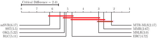
Figure 3.
Bonferroni–Dunn test with comparisons of MTR-MLS against other compared methods.
As can be seen in Figure 3, although MTR-MLS is not significantly different from MMR and MSLR for all datasets, there is a significant improvement in performance between the above algorithms and other MTR algorithms. Because these algorithms consider the correlation between different target outputs and impose sparsity constraints in the modelling process, which makes they are significantly superior to the problem transformation algorithms (SST, RLC and ERC) on different datasets. Furthermore, these algorithms are based on the multi-layer sparse latent variable regression framework, which can make full use of the correlation information between different outputs to obtain better prediction results than mSVR, which only considers multiple output errors, and OKL, which only considers the positive correlation between targets. The MTR-MLS algorithm maintains better performance than MMR and MSLR on the datasets with a high number of output targets (OES10, OES97, OSALES, SCM1d, SCM20d, WQ), indicating that the proposed algorithm can learn the complex structured noises by sparse learning of the complex structured noise among the targets of the datasets.
4.3. Experiments in Cost Prediction of WMS
In order to verify the effectiveness of this method in the application of WSM cost prediction, the cost data of WSM are studied. In the WSM cost data collection, we collected all repair records from different undertaking factories for different types of warships in the past five years, including the basic information of the repaired warship and undertaking factory. The collected index system of WSM maintenance incidents is shown in Figure 4.
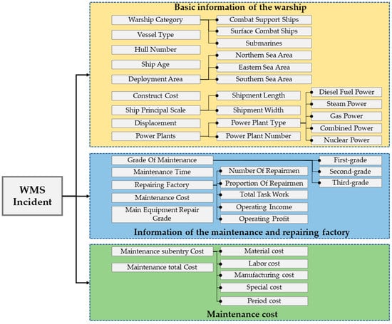
Figure 4.
Index system of WSM maintenance incidents.
As is shown in Figure 4, the maintenance cost is not only related to the performance parameters of the warship, but also to the context of the maintenance such as the factory of the maintenance, and the maintenance time. Based on the index system shown in Figure 4, the input–output characteristic feature sets shown in Table 3 is constructed, where the input feature set is the quantifiable basic information index of the warship collected and various indexes related to the repairing factory, and the output corresponds to the subentry costs of WSM. In Table 3, the power unit type (C5) and the maintenance unit (C10) are one-hot encoded. Hence, the input dimension of the sample set after pre-processing is 23, and the output target number is 5.
Table 3.
Feature sets for WSM cost prediction.
In order to ensure a good similarity between the WSM samples or events involved in the prediction, the sample set is preliminarily divided into multiple datasets according to the warship type (combat support warships, surface combat warships and submarines) and maintenance grade (second-grade and third-grade maintenance, because there are few instances of first-grade maintenance, so it is not considered). Then, considering the similarity of WSM cost data in distance and angle, define the similarities between the maintenance instance and as follows:
Formula (25) clusters the instances by using the hybrid similarity function based on the angle cosine and the Euclidean distance and obtains several representative instances sets of WSM. As shown in Table 4, the WSM dataset with different ship categories and maintenance grades are obtained by nearest neighbour clustering [42] based on the similarity function (25), to ensure good similarity among different samples under the same datasets. After normalizing the input and output features of the datasets, the MTR-MLS algorithm is applied, and the performance of the MTR-MLS-based cost prediction model on the test set is tested by a five-fold cross-validation.
Table 4.
Description of the WSM datasets.
The optimal parameter settings corresponding to the MTR-MLS algorithm for different datasets are given in Table 5, and the performance results of the algorithm on different subentry costs are shown in Table 6.
Table 5.
Parameter settings corresponding to the MTR-MLS algorithm for different WSM datasets.
Table 6.
MAPE(%) values of MTR-MLS algorithm on WSM datasets.
In Table 6, the test errors for different maintenance grades do not differ much. Among them, the prediction accuracy of manufacturing cost (D3) and period cost (D5) is around 12%, which is significantly better than the prediction results of the other three subentry costs. This is because the variability in maintenance time between WSM tasks of the same category and grade is not significant, and the fluctuations in manufacturing and period costs are smaller. Therefore, it is reasonable to estimate the manufacturing and period costs of new events based on historical data of the same category and grade of WSM.
In order to better compare the prediction accuracy of itemized cost with the total cost, the final total cost prediction is obtained by inverse-normalization based on the prediction results of the algorithm on subentry cost in Dataset 4. Similarly, based on the same strategy, we adopt the representative multi-output support vector regression (mSVR) and BPNN to predict the total cost of secondary maintenance of surface combatant ships. In BPNN, the topology was set as 23-15-5. Sigmoid and purelin were exploited as the activation function and in the hidden layer and the transfer function in the output layer, respectively. We set the maximum number of convergences as 150, while the learning rate and the error equaled 0.1 and 0.001, respectively. In mSVR, the penalty parameter c and kernel parameter σ were grid search in interval [10−3, 103]. The prediction results of some samples in Dataset 4 are shown in Table 7.
Table 7.
Comparison of total cost prediction results of three different algorithms in Dataset 4 (unit: million yuan).
The predicted values of the different methods for samples in dataset 4 in terms of total costs and the corresponding errors are shown in Figure 5. In particular, the predicted values of the WSM samples’ total costs are obtained by summing the predicted subentry cost values. The total cost prediction results obtained by summing multiple subentry costs of WSM using the proposed MTR method are significantly better than the traditional multi-output algorithms such as mSVR and BPNN. This indicates that by exploring the correlation knowledge among different subentry costs, the prediction accuracy of WSM cost can be effectively improved.
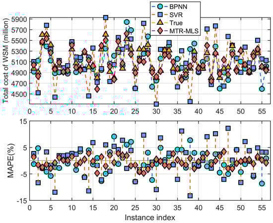
Figure 5.
The results of three methods for predicting the total cost of WSM.
The scatter plot in Figure 6 depicts the fitting results of the sample within dataset 4, with the horizontal and vertical coordinates of the points representing its actual total cost and the predicted total cost value obtained from the model prediction, respectively. It is evident that compared with other multi-output approaches, the prediction errors of the proposed method in this paper are less volatile, which indicates that the prediction results of the method are more stable and less susceptible to the interference of outliers.
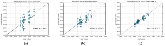
Figure 6.
Comparison of predicted and actual values of total WSM costs for different methods: (a) Prediction results based on mSVR; (b) Prediction results based on BPNN; (c) Prediction results based on MTR-MLS.
5. Conclusions
In this paper, we propose the MTR-MLS algorithm to handle the task of predicting the subentry cost of WSM. By incorporating a latent space and auxiliary matrix, the MTR-MLS can explicitly encode the inter-target correlations and structure noises in structure and auxiliary matrices. Experimental results on both the real-world datasets and WSM cost datasets have shown that the MTR-MLS achieves high performance and outperforms the traditional multi-output representative algorithms, which indicates its effectiveness for predicting the subentry costs of WSM.
However, there are still some shortcomings in this paper, which need to be improved in subsequent research: First, this paper only constructs the hybrid similarity function and uses the clustering method to classify different WSM events, but does not investigate the data information correlation between different events. This also limits the performance of the algorithm. Moreover, it is very important for WSM cost forecasting. Thus, a new feature selection method will be a research focus in the future.
Author Contributions
Data curation, formal analysis, writing—original draft, writing—review and editing, D.H.; supervision, investigation, validation, S.S.; project administration, resources, methodology, software, visualization, L.X. All authors have read and agreed to the published version of the manuscript.
Funding
This research was funded by the National Social Science Foundation of China, grant number 18BGL287, 19CGL073.
Institutional Review Board Statement
Not applicable.
Informed Consent Statement
Not applicable.
Data Availability Statement
The data that has been used is confidential.
Acknowledgments
The authors would like to thank Zhang Kan for his fund support.
Conflicts of Interest
The authors declare no conflict of interest.
References
- Lin, M.; He, D.; Sun, S. Multivariable case adaptation method of case-based reasoning based on multi-case clusters and Multi-output support vector machine for equipment maintenance cost prediction. IEEE Access 2021, 9, 151960–151971. [Google Scholar] [CrossRef]
- Zhang, Q. Prediction of ship equipment maintenance cost based on grey relational degree and SVM. Comput. Digit. Eng. 2010, 38, 15–18. [Google Scholar] [CrossRef]
- Shang, F.; An, T.; Xie, L.; Sun, S. Grey combination prediction model for calculating target price of equipment repair. J. Wuhan Univ. Technol. (Inf. Manag. Eng. Ed.) 2015, 37, 497–501. [Google Scholar]
- Liu, M. Application of improved GM (1,1) model in ship maintenance cost prediction. Ship Electron. Eng. 2010, 30, 151–154. [Google Scholar]
- Liu, L.; Geng, J.; Wei, S.; Xu, S. Analysis of factors affecting ship equipment maintenance costs based on grey orthogonal. Firepower Command Control 2018, 43, 89–93. [Google Scholar]
- He, P.; Sun, S. Prediction model of ship equipment maintenance cost based on improved GM (0, N). Ship Electron. Eng. 2022, 42, 151–154. [Google Scholar]
- Yin, S.; Xie, N.; Hu, C. Development cost estimation of civil aircraft based on combination model of GM (1, N) and MLP neural network. In Proceedings of the 2015 IEEE International Conference on Grey Systems and Intelligent Services (GSIS), Leicester, UK, 18–20 September 2015; pp. 312–317. [Google Scholar]
- Zi, S.; Wei, R.; Jiang, T.; Xie, L. Improved adjustment model of ship maintenance cost cases. Syst. Eng. Electron. Technol. 2012, 34, 539–543. [Google Scholar]
- Zi, S.; Wei, R.; Jiang, T.; Xie, L. Application of case-based reasoning in prediction of ship maintenance costs. J. Nav. Univ. Eng. 2012, 24, 107–112. [Google Scholar]
- Zi, S.; Wei, R.; Guan, B.; Xie, L.; Jiang, T. Case similarity retrieval technology in ship maintenance cost prediction. Comput. Integr. Manuf. Syst. 2012, 18, 208–215. [Google Scholar]
- Lin, M.; Wang, C.; Xie, L. Case based reasoning prediction of ship equipment maintenance cost based on double similarity retrieval. J. Nav. Univ. Eng. 2022, 34, 68–73. [Google Scholar]
- Lin, M.; Wang, C.; Tang, Z. Prediction method of ship planned maintenance cost based on case based reasoning. China Ship Res. 2021, 16, 72–76. [Google Scholar]
- Kasie, F.; Bright, G. Integrating fuzzy case-based reasoning, parametric and feature-based cost estimation methods for machining process. J. Model. Manag. 2021, 16, 825–847. [Google Scholar] [CrossRef]
- Jian, T.; Zhong, Q.; Jin, B. Study on Cost Forecasting Modeling Framework Based on KPCA & SVM and a Joint Optimization Method by Particle Swarm Optimization. In Proceedings of the 2009 International Conference on Information Management, Innovation Management and Industrial Engineering, Washington, DC, USA, 26–27 December 2009; pp. 375–378. [Google Scholar]
- Jian, T.; Zhang, H. Study on Cost Prediction Modeling with SVM Based on Sample-Weighted. In Proceedings of the 2010 3rd International Conference on Information Management, Innovation Management and Industrial Engineering, Kunming, China, 26–28 November 2010; pp. 477–480. [Google Scholar]
- Ibrahim, E.-S.N. Support Vector Machine Cost Estimation Model for Road Projects. J. Civ. Eng. Archit. 2015, 9, 1115–1125. [Google Scholar]
- Chou, J.-S.; Cheng, M.-Y.; Wu, Y.-W.; Tai, Y. Predicting high-tech equipment fabrication cost with a novel evolutionary SVM inference model. Expert Syst. Appl. 2011, 38, 8571–8579. [Google Scholar] [CrossRef]
- Chen, X.; Yi, M.; Huang, J. Application of a PCA-ANN Based Cost Prediction Model for General Aviation Aircraft. IEEE Access 2020, 8, 130124–130135. [Google Scholar] [CrossRef]
- Wang, H.; Huang, Y.; Gao, C.; Jiang, Y. Cost Forecasting Model of Transformer Substation Projects Based on Data Inconsistency Rate and Modified Deep Convolutional Neural Network. Energies 2019, 12, 3043. [Google Scholar] [CrossRef]
- Ujong, J.; Mbadike, E.; Alaneme, G. Prediction of cost and duration of building construction using artificial neural network. Asian, J. Civ. Eng. Build. Hous. 2022, 23, 1117–1139. [Google Scholar] [CrossRef]
- Papatheocharous, E.; Andreou, A. Hybrid Computational Models for Software Cost Prediction: An Approach Using Artificial Neural Networks and Genetic Algorithms; Springer: Berlin/Heidelberg, Germany, 2009. [Google Scholar]
- Liu, G.; Tang, X.; Liu, Y. Prediction for Missile Development Cost Based on Neural Network. Tactical Missile Technol. 2003, 1, 23–26. [Google Scholar]
- Liu, J.; Ye, Q. Xiamen Project Cost Prediction Model Using BP and RBF Neural Networks. J. Overseas Chin. Univ. Nat. Sci. Ed. 2013, 34, 576–580. [Google Scholar]
- Borchani, H.; Varando, G.; Bielza, C.; Larrañaga, P. A survey on multi-output regression. WIREs Data Min. Knowl. Discov. 2015, 5, 216–233. [Google Scholar] [CrossRef]
- Spyromitros-Xioufis, E.; Tsoumakas, G.; Groves, W.; Vlahavas, I. Multi-Label Classification Methods for Multi-Target Regression. Comp. Sci. 2012, 104, 55–98. [Google Scholar]
- Tsoumakas, G.; Spyromitros-Xioufis, E.; Vrekou, A.; Vlahavas, I. Multi-Target Regression via Random Linear Target Combinations; Springer: Berlin/Heidelberg, Germany, 2014; pp. 225–240. [Google Scholar]
- Zhen, X.; Yu, M.; He, X.; Li, S. Multi-Target Regression via Robust Low-Rank Learning. IEEE Trans. Pattern Anal. Mach. Intell. 2018, 4, 497–504. [Google Scholar] [CrossRef] [PubMed]
- Evgeniou, T.; Micchelli, C.; Pontil, M. Learning Multiple Tasks with Kernel Methods. J. Mach. Learn. Res. 2005, 6, 615–637. [Google Scholar]
- Dinuzzo, F. Learning output kernels for multi-task problems. Neurocomputing 2013, 118, 119–126. [Google Scholar] [CrossRef][Green Version]
- Arashloo, S.R.; Kittler, J. Multi-target regression via non-linear output structure learning. Neurocomputing 2022, 492, 572–580. [Google Scholar] [CrossRef]
- Dinuzzo, F.; Ong, C.; Gehler, P.; Pillonetto, G. Learning Output Kernels with Block Coordinate Descent. In Proceedings of the 28th International Conference on Machine Learning (ICML-11), Washington, DC, USA, 28 June–2 July 2011. [Google Scholar]
- Mauricio, A.; Lorenzo, R.; Neil, D. Kernels for Vector-Valued Functions: A Review. Found. Trends® Mach. Learn. 2012, 4, 195–266. [Google Scholar]
- Rai, P.; Kumar, A.; Daumé, H. Simultaneously leveraging output and task structures for multiple-output regression. In Proceedings of the 25th International Conference on Neural Information Processing Systems—Volume 2; Curran Associates Inc.: Lake Tahoe, NV, USA, 2012; pp. 3185–3193. [Google Scholar]
- Zhen, X.; Yu, M.; Zheng, F.; Nachum, I.B.; Bhaduri, M.; Laidley, D.; Li, S. Multitarget Sparse Latent Regression. IEEE Trans. Neural Netw. Learn. Syst. 2018, 29, 1575–1586. [Google Scholar] [CrossRef]
- Zhang, Y.; Yeung, D.-Y. A convex formulation for learning task relationships in multi-task learning. In Proceedings of the Twenty-Sixth Conference on Uncertainty in Artificial Intelligence; AUAI Press: Catalina Island, CA, USA, 2010; pp. 733–742. [Google Scholar]
- Dinuzzo, F.; Schölkopf, B. The Representer Theorem for Hilbert Spaces: A Necessary and Sufficient Condition; Curran Associates Inc.: Red Hook, NY, USA, 2012. [Google Scholar]
- Tsoumakas, G.; Spyromitros-Xioufis, E.; Vilcek, J.; Vlahavas, I. MULAN: A Java Library for Multi-Label Learning. J. Mach. Learn. Res. 2011, 12, 2411–2414. [Google Scholar]
- Sanchez-Fernandez, M.; de-Prado-Cumplido, M.; Arenas-Garcia, J.; Perez-Cruz, F. SVM Multiregression for Nonlinear Channel Estimation in Multiple-Input Multiple-Output Systems. IEEE Trans. Signal Process. 2004, 52, 2298–2307. [Google Scholar] [CrossRef]
- Gong, P.; Ye, J.; Zhang, C. Robust Multi-Task Feature Learning, KDD: Proceedings. Int. Conf. Knowl. Discov. Data Min. 2012, 2012, 895–903. [Google Scholar]
- Herrera, S.G.i.F. An Extension on “Statistical Comparisons of Classifiers over Multiple Data Sets” for all Pairwise Comparisons. J. Mach. Learn. Res. 2008, 9, 2677–2694. [Google Scholar]
- Demsar, J. Statistical Comparison of Classifiers over multiple dataset. J. Mach. Learn. Res. 2006, 7, 1–30. [Google Scholar]
- Qi, J.; Hu, J.; Peng, Y. A new adaptation method based on adaptability under k-nearest neighbors for case adaptation in case-based design. Expert Syst. Appl. 2012, 39, 6485–6502. [Google Scholar] [CrossRef]


Disclaimer/Publisher’s Note: The statements, opinions and data contained in all publications are solely those of the individual author(s) and contributor(s) and not of MDPI and/or the editor(s). MDPI and/or the editor(s) disclaim responsibility for any injury to people or property resulting from any ideas, methods, instructions or products referred to in the content. |
© 2022 by the authors. Licensee MDPI, Basel, Switzerland. This article is an open access article distributed under the terms and conditions of the Creative Commons Attribution (CC BY) license (https://creativecommons.org/licenses/by/4.0/).